Article

Long-Term Yield and Quality Performance of Perennial Energy Grasses (Agropyron spp.) on Marginal Land

1
CEDER-CIEMAT—Centro de Desarrollo de Energías Renovables, Autovía Navarra A-15, Salida 56, 42290 Lubia (Soria), Spain
2
Departamento de Producción Agraria, Universidad Politécnica de Madrid (UPM), 28040 Madrid, Spain
*
Author to whom correspondence should be addressed.
Agronomy 2020, 10(7), 1051; https://doi.org/10.3390/agronomy10071051
Submission received: 7 June 2020 / Revised: 16 July 2020 / Accepted: 20 July 2020 / Published: 21 July 2020
(This article belongs to the Special Issue Sustainable Management and Utilization of Permanent Grassland)

Abstract

:
The cultivation of perennial grasses is one of the most desirable alternatives as energy feedstock, but it is difficult to achieve competitive yields under Mediterranean marginal conditions. The aim of this study was to assess the performance of three cool-season grasses (Agropyron spp.) from an agronomic and energetic point of view by comparing the dry matter (DM) yields, rain use efficiency, chemical composition, and biomass quality over an eight-year period in Spain under marginal rainfed conditions. The tall wheatgrass (Agropyron elongatum (Host) Beauv.) cultivars, Alkar (4.8 Mg DM·ha−1) and Jose (4.7 Mg DM·ha−1), achieved the highest yields. Productions below 0.5 Mg DM·ha−1 were obtained when rainfall was lower than 150 mm between March and June. The biomass obtained from the tested grasses showed relatively high contents of ash, silicon, and alkali elements. Net calorific values ranged between 16.7 and 18.5 MJ·kg−1 db. Differences in the composition among species and cultivars are not likely to affect their combustion behavior from a practical point of view. The ash content, as well as the concentrations of K, S, Na, and Cl, tended to decrease over the years. The results offered would be very useful for the implementation of this type of crop in marginal land.

1. Introduction

The optimism regarding the potential of biofuels as an alternative to fossil fuels was high at the beginning of the 21st century [1]. Benefits, such as greenhouse gases (GHG) emission reduction, heat, electricity de-carbonization, and the development of rural areas, were expected for biofuel use [2]. However, there is speculation regarding the contribution of biofuels to the increase of food prices and the use of freshwater [3,4]. This raised important issues regarding the use of arable lands for growing crops dedicated to biofuel production [5,6,7] and it created a conflict between both alternatives [8].
In this context, marginal lands have been revealed as an important source of land for growing energy crops [7]. Marginal lands are areas where it is difficult to grow food crops profitably given the conditions that exist at the site, the agricultural policies and available growing methods, as well as the global or national economic situations [9,10]. According to the European Environmental Agency (EEA), marginal land is “a low-quality land whose production barely covers its cultivation costs”. The United States Department of Agriculture (USDA) defines marginal lands as “in farming, poor quality land that is likely to yield a poor term return”. Those lands are therefore characterized by low food and feed productivity associated with socio-economic and biophysical constraints [11,12].
The uses of perennial grasses have been widely reported as the best alternative for producing biomass in marginal lands in agronomic, economic, and environmental terms. Perennial grasses compared to traditional annual crops reduce soil nutrient depletion and soil erosion, require a low input for their production and provide a better profit margin, increase soil quality and carbon sequestration, enhance the agricultural ecosystems’ biodiversity by avoiding the mono-cropping and providing protection and feed to wild fauna (mammals, birds and insects), and increase soil water retention [13,14,15,16,17,18,19,20,21,22,23,24,25,26,27,28,29]. The perennial grasses most used for producing biomass in Europe and the US are miscanthus (Miscanthus giganteus Greef et Deuter), giant reed (Arundo donax L.), switchgrass (Panicun virgatum L.), and reed canary grass (Phalaris arundinacea L.), but implanting them under marginal conditions is not recommended due to their soil and water requirements [30]. In turn, perennial cool-season grasses can be alternative bioenergy crops for sustainable biomass production on marginal lands generally not suited to grain crop production [31,32]. In particular, tall wheatgrass, crested wheatgrass (Agropyron cristatum (L.) Gaertn.), and Siberian wheatgrass (Agropyron sibiricum (Willd.) P. Beauv.) possess characteristics that can be useful in marginal lands. These species share similar traits regarding their salinity and drought tolerance, winter frost hardiness, and resistance to pests and illnesses [33,34,35], in addition to the rest of the advantages described above for being perennial grasses. All of them are cool-season grasses that have been traditionally used as pastures for grazing or for obtaining hay [36].
Many studies around the world provide information on yields and the quality of these grasses in terms of forage production for animals [36,37], while others show the production and quality of the biomass of different varieties on fertile arable land or grasslands [38,39,40,41]. However, very scarce information is available on the use of these Agropyron species as combustion feedstock on arable lands under marginal conditions. The composition and the combustion behavior of grass biomass are strongly influenced by crop management and developmental stage but also depend on the species considered and on site factors, such as soil characteristics and weather conditions [30,42,43]. The literature shows how the composition of cool-season grasses differs greatly within and among different locations [30,44,45], and they can thus have considerably different amounts of certain “anti-quality” minerals like Cl, K, Si, N, or S that cause emissions, slagging, and/or corrosion at the operating temperatures of combustion plants [30,42,43,45,46]. For all these reasons, it is important to clarify from a productive and a quality perspective whether or not cool-season grasses can be a long-term sustainable resource for energy feedstock under marginal conditions.
In the above context, the main aim of this study was to evaluate three species of Agropyron spp. from an agronomic and energy perspective, comparing their biomass yield, composition, and quality in a low productive agricultural area under rainfed conditions. One cultivar (cv.) of crested wheatgrass (Hycrest), one cultivar of Siberian wheatgrass (Vavilov II), and three cultivars of tall wheatgrass (Alkar, Jose, and Riparianslopes) were tested for eight years in a marginal location, while another three tall wheatgrass cultivars (Alkar, Bamar, and Szarvasi-1) were tested for five years in a second marginal location. These results are of key importance for determining the commercial future of these crops as a feedstock for energy production when growing under marginal conditions.

2. Materials and Methods

2.1. Experimental Sites

The study was carried out in two different locations of Spain’s North-Central Plateau, one of the most extended areas of rainfed agriculture in southern Europe. The experimental fields were located in Cubo de la Solana (CS) [41° 36′ N and 2° 28′ W], 1010 m above sea level, and in Alconaba (AL) [41° 42′ N and 2° 22′ W], 1000 m above sea level.
Experimental fields were located in areas with severe biophysical limitations [47]. In both places, soils were poor and sandy (81% of sand in the CS fields and 88% of sand in the AL fields), with a content of coarse elements (>2 mm) higher than 15% in soil volume. Soils were characterized by low levels of organic matter (≤1%), and low water and nutrient retentions, indicating potential high losses by leaching. Soils were pH neutral and did not exhibit salinity problems. Soil nitrogen content was 0.06% in the CS plots and 0.03% in AL; the content in phosphorus (P2O5) was 10.2 and 10.0 mg·kg1 in CS and AL, respectively; and the content of the soil in potassium (K2O) was 152.5 mg·kg1 in the CS fields and 150 mg·kg1 in the AL plots. Soil samples were taken from the upper layer (0–30 cm) as indicated in ISO 10381-1, and analyzed according to ISO standards for texture (ISO 11277), pH (ISO 10390), electrical conductivity (ISO 11265), organic matter (ISO 10694), phosphorus (ISO 11263), potassium (ISO 11260), and ammonium and nitrates (ISO/TS 14256-1 EX).
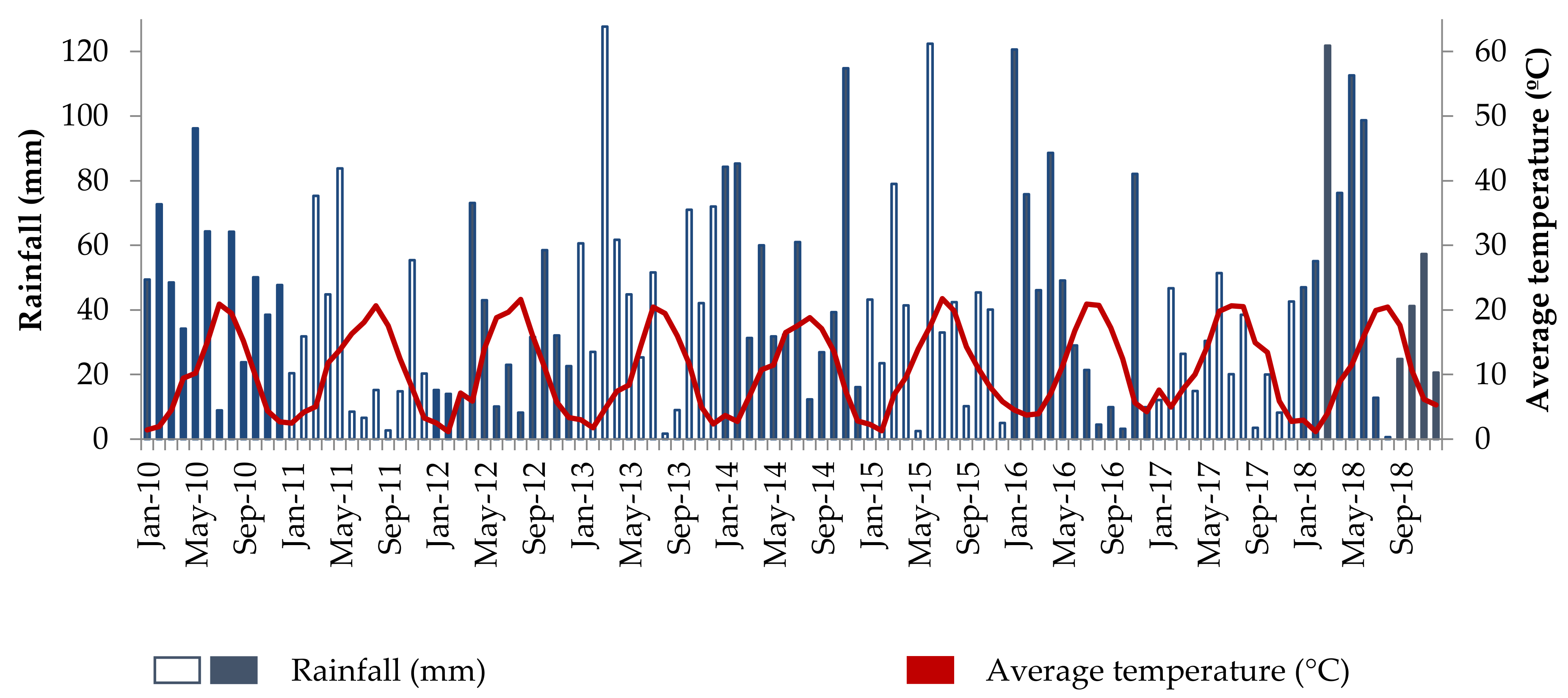
Climate conditions were continental Mediterranean with cold winters, warm summers, and low rainfall levels. Climate data were taken from the nearest national grid of meteorological stations. The average annual rainfall during the study period was 502.7 mm in the CS fields, with 2018 being the wettest year (669 mm) and 2017 the driest (315 mm). Harvesting was hardly possible in 2017 due to the extremely low biomass production obtained as a consequence of the low annual precipitation registered at this location, particularly between March and June (123 mm). The annual average temperature was 10.6 °C, with minimum and maximum absolute temperatures of −11.9 °C in January 2011 and 37 °C in August 2012, respectively. The free frost period was from late May to early October, and drought conditions usually appeared during the summer. Figure 1 shows the monthly rainfall and average temperatures during the study period in the CS experimental trials.
The AL fields registered 437 mm of annual average rainfall, with 2018 being the wettest year (524 mm) and 2017 the driest with 351 mm. The annual average temperature was 10.5 °C, and the minimum and maximum absolute temperatures were −10.5 °C in January 2017 and 36.01 °C in July 2015, respectively. AL exhibited the same frost and drought periods as CS. Figure 2 depicts the monthly rainfall and average temperatures.

2.2. Experimental Design and Crop Management

CS field trials were studied for 8 years (October 2010–August 2018). The experiment in the CS fields was designed by sowing three repetitions in a randomized complete block design in 300-m2 plots (3 m wide × 100 m long) for each experimental unit. As it was commented previously, the varieties sown were tall wheatgrass (cv. Alkar (TWA), cv. Jose (TWJ), cv. Riparianslopes (TWR)), crested wheatgrass (cv. Hycrest) (CWH), and Siberian wheatgrass (cv. Vavilov) (SWV).
In the AL fields, 3 cultivars of tall wheatgrass were sown with 4 repetitions for 5 years (October 2013–August 2018) in plots with a similar surface area, shape, and design as the CS fields. The cultivars sown in the AL experiment were tall wheatgrass (cv. Alkar (TWA), cv. Bamar (TWB), and cv. Szarvasi-1 (TWS)).
The previous crop in both trials was fallow land. It was plowed seven months earlier, cultivated in summer, and sown in October (2010 in the CS fields and 2013 in Al plots). The seeding dose was 20 kg·ha−1 for tall wheatgrass cultivars and 15 kg·ha−1 for crested wheatgrass and Siberian wheatgrass, with a seeding drill in rows 13 cm apart. A complex fertilizer NPK 8-24-8 (300 kg·ha−1) was applied for base fertilization in the establishment year. Base fertilization was applied two days before sowing and buried with a cultivator. In addition, plots were rolled in mid-March in the establishment year, prior to the application of the top fertilization. Experimental plots were sprayed in late April for controlling broadleaves weeds with 1 L·ha−1 of 2.4-D acid 34.5% + 2-methyl-4-chlorophenoxyacetic acid 34.5%. Nitrogen fertilizer was applied as top dressing between mid- and late-March every year using nitrogen (27% purity) at 300 kg·ha−1·y−1. Crops were harvested with a mower conditioner from mid-July to early August depending on the year, always when crops were in the doughy grain stage and leaving 10 cm of stubble to encourage further regrowth. After 5 to 6 days of field drying, biomass was baled in prismatic bales (<10% moisture).
The main limiting factor for plant growth under rainfed conditions is water availability. Biomass production of crops depends on their efficiency in water use. Hence, crops with better efficiency also achieve a better economic margin. The cited efficiency is often expressed as water-use efficiency (WUE) or rain-use efficiency (RUE), and it is measured in terms of crop production per unit of water input. Specifically, RUE = yield (g DM·ha−1)/rainfall occurred (l) [48]. Although WUE and RUE have been primarily evaluated in traditional agronomic crops, they can also impact the potential of crops for cellulosic biofuels [49]. The RUE was calculated to assess the differences among cultivars and species. The calculation period occurred in the months with the highest vegetative activity (March to June), which is when rainfall is considered to be of key importance for biomass production in cool-season grasses under rainfed conditions, as other authors reported [48,50].

2.3. Experimental Characteristics and Analytical Methods

Sample preparation was performed according to ISO 14780:2017 [51] and test analyses were carried out following the corresponding international standards for solid biofuels (Table 1).
Bales were weighed with a laboratory scale in the fields. Moisture content was measured by oven-drying subsamples in an oven at 40 °C until constant weight. Dry matter yields were calculated by taking into account the plot area, as well as the weight and moisture content of the bales.
Before baling, a combined sample per replicate plot, cultivar, and year was analyzed to determine the main properties and the chemical composition of the biomass. Every combined sample was formed by manually collecting 3 subsamples from different random locations in the replicate plot and leaving the same stubble as the mower did. Biomass from CS fields was analyzed for 7 years from 2012 until 2018. The biomass from the establishment year was not analyzed. Biomass from the AL plots was analyzed annually between 2014 and 2018.
Major elements were analyzed by digesting the ashes of the biomass obtained at 550 °C (ISO 18122:2015), followed by ICP-OES determination according to ISO 16967:2015. Results were expressed in biomass dry basis (db). Titanium contents were very low and frequently below the method quantification limit (<0.0002%), and thus the results obtained for this element are not shown or treated statistically. Calorific values were analyzed by calorimetry (ISO 16994:2016) and expressed as the gross calorific value at constant volume (GCVv,o) and net calorific value at constant pressure (NCVp,o), both in db.
A number of fuel predictive indices and ratios between chemical elements were calculated to predict the combustion behavior of the biomass cultivated. These indices were selected from the literature because they were previously used as a measure of the quality of other herbaceous biofuels for combustion.
In this sense, the ratio between the earth alkaline oxides and alkaline oxides (AE/A), the ratio between the content of K and the sum of Ca and Mg [K/(Ca + Mg)], as well as the molar ratio between the sum of Si, P, and K and the sum of Ca and Mg [(Si + P + K)/(Ca + Mg)] were used as indicators of problems related to ash sintering and fusion.
AE/A is calculated by dividing the concentrations of CaO and MgO and the concentrations of K2O and Na2O in the ash fuel [52]. Solid biofuels with AE/A ratios over 2 have been associated with a lower risk of ash sintering in a 1 MWth bubbling fluidized bed combustion pilot plant [52].
The K/(Ca + Mg) ratio was used as an indicator of slagging for the thermo-chemical processing of grasses [53]. It was estimated that grasses with ratios below 0.5 did not pose issues regarding ash sintering or ash fusion, e.g., in operational gasifiers [53].
A linear correlation between the ash sintering temperature (SST) and the molar ratio (Si + P + K)/(Ca + Mg) was also empirically demonstrated for P and K-rich fuel ash systems [54,55]. Zeng et al. did find a good correlation between SST and pellets produced from blends of miscanthus, a warm-season grass, with wood and wheat straw [55]. Fuels with lower (Si + P + K)/(Ca + Mg) molar ratios tend to exhibit higher ash sintering temperatures [54]. Fuels with indices below 1 and 3 are expected to exhibit SSTs equal to or higher than 1200 and 1000 °C, respectively [54].
The sum of K + Na + Zn + Pb can be used as an indicator of PM1 emissions [54]. Low PM1 emissions are expected for indices below 1000 mg kg−1. In turn, fuels with indices over 10,000 mg kg−1 tend to cause high PM1 emissions [54]. As trace elements were not determined in this study, a Pb content of 1 mg kg−1 was used to calculate this index, based on previous experimental trials where the biomass of tall wheatgrass was analyzed in these regions.
The molar Si/K ratio was used to predict aerosol formation during the combustion of grasses, among other fuels [54,56]. A high molar Si/K ratio can lead to a preferred formation of potassium silicates in the bottom ash, resulting in a lower K release and aerosol formation, but gaseous SOx and HCl emissions may increase [54].
The molar ratio (K + Na)/[x(2S + Cl)] was used to predict SOx and HCl emission levels [54,55]. In this study, an x factor of 4.9 was used to calculate this index, as this is the value that was experimentally determined by Sommersacher et al. for Arundo donax, also a cold-season grass perennial. For fuels with high molar ratios, S and Cl will be preferably embedded in the ashes, forming alkaline sulfates and chlorides, potentially resulting in low SOx and HCl emission levels [54,55].
The 2S/Cl molar ratio has been used as an indicator for high-temperature corrosion risks [54]. Fuels with ratios below 2 are expected to pose a severe risk. Minor risks are expected when ratios are >4. In turn, for 2S/Cl ratios <2, severe corrosion risks need to be taken into account, as a result of a high Cl surplus in aerosols [54].

2.4. Statistical Analysis

Statistical analyses were performed using the Statgraphics Centurion XVII (Statpoint Technologies INC, 2017, The Plains, VA, USA) software. The effects of the different species (S), cultivars (C), and years (Y) on biomass production and composition as well as on empirical fuel indices were evaluated by means of the variance analysis (ANOVA). Multifactorial two-way ANOVAs (Type III sums of squares) with a maximum order interaction of 2 were used. All F-ratios were based on the residual mean square error. The normality of the data and the homoscedasticity of variances were verified using the standardized skewness/kurtosis and Levene’s test, respectively. No data transformations were considered necessary. In AL fields, C, Y, and the interaction between both factors (C × Y) were considered to be fixed effects. In CS fields, two types of analysis were performed as different species and cultivars were tested. On the one hand, an analysis of variance with S, Y, and S × Y as fixed effects, with the factor species at three levels (tall wheatgrasses—TW, crested wheatgrass—CW, and Siberian wheatgrass—SW). On the other hand, an analysis of variance with species/cultivars (S/C), Y, and their interaction (X/C × Y) as fixed effects, and considering five levels for factor S/C (TWR, TWA, TWJ, CWH, and SWV) was conducted. Block (replicate plots) was considered a random effect at both sites. Mean differences across species, cultivars, and years were assessed using multiple range tests according to the Fisher’s least significant difference (LSD) test. Significant effects were revealed at p-values ≤0.05 (95% of confidence level). Interactions among factors (species and years or cultivars and years) were depicted by using the means and Fisher´s LSD interaction plots. Means, standard deviations (SD), 75% percentiles (P75), as well as minimum and maximum individual values obtained for each property were also included in their corresponding tables.

3. Results

3.1. Biomass Yield and Rain Use Efficiency

According to the results obtained (Table 2), significant effects of species, cultivars, and years were found in biomass production at both experimental areas. RUE also had significant effects across species, cultivars, and years at both locations.
Biomass yields from the CS and AL fields are shown in Table 3. In CS fields, the year with the highest production was 2018 (9.8 Mg DM·ha−1 average value), with tall wheatgrass cv. Jose being the most productive species with 12.6 Mg DM·ha−1. It should also be mentioned that the lowest biomass productions were achieved during the previous year (2017), due to the extremely low precipitation levels registered, especially in spring, which even made baling difficult with the technology used in this study. Additionally, low yields were also obtained during the establishment year (1.7 Mg DM·ha−1). When taking into account the whole study period (2011–2018), TWA and TWJ provided the highest yields, with annual average productions of 4.8 and 4.7 Mg DM·ha−1, respectively. In turn, CWH provided the lowest annual yields (2.8 Mg DM·ha−1).
In the AL plots, the best yields were obtained in 2018 (4.9 Mg DM·ha−1) and 2015 (4.7 Mg DM·ha−1), the latter due to the good performance of TWS (7 Mg DM·ha−1 in 2015). In general, the lowest yields were achieved during the establishment year (1.9 Mg DM·ha−1), which were close to those registered in 2017 (2.8 Mg DM·ha−1), the one with the lowest annual rainfall. TWS provided the highest average annual yields (4.3 Mg DM ha−1), followed by TWB (3.5 Mg DM ha−1) and TWA (3.0 Mg DM ha−1). It is also worth mentioning that the TWS cultivar achieved better results during the first years of the experiment while TWA performed better later on.
All tall wheatgrass cultivars tested in CS showed a more efficient rainfall use (around 2.0 g DM·L−1) (Table 4) than crested and Siberian wheatgrass, which provided lower biomass yields for the same precipitation. Comparing years, the best rain efficiency was in 2013 and 2018 (2.6 g DM·L−1 and 2.4 g DM·L−1, respectively). Similar rain efficiencies were achieved in 2014 and 2015. In connection with biomass production, 2017 was the year with the lowest rainfall efficiency due to the low precipitation registered during the period with the highest vegetative activity (123 mm). In the AL fields, TWS was the cultivar with the highest RUE (2.2 g DM·L−1), differing from TWA (1.4 g DM·L−1), the latter being the one with the lowest RUE.

3.2. Biomass Composition

The statistical significance of the factors considered (species, cultivars, and years) and their corresponding interactions in the biomass properties and chemical composition of the grasses cultivated at both sites (CS and AL) are listed in Table 5. The main properties and chemical composition of the different perennial grasses cultivated in CS during the 2011-2018 harvest period are shown in Table 6 and Table 7. As explained in Section 2.1, CWH, SWV, and three tall wheatgrass cultivars (TWA, TWJ, and TWR) were tested. Results for the three tall wheatgrass cultivars tested in the AL experimental trials (TWA, TWB, and TWS, see Section 2.1) from harvest 2013 to harvest 2018 are listed in Table 8 and Table 9. These tables include the mean values for three replicate plots per species, cultivar, and year (Table 6, Table 7, Table 8, Table 9).
As can be seen in Table 5, the species and cultivars tested in the CS fields differed significantly in their calorific value, ash, C, H, K, Mg, Na, Si, and Zn contents. No significant differences were found in their N, S, Cl, Al, Ca, Fe, Mn, and P contents.
For all the properties with p-values below 0.05 for the S/C factor, the main differences were found across species rather than among cultivars. In this sense, tall wheatgrass showed significant differences with respect to the other wheatgrass species tested (crested and Siberian), while all tall wheatgrass cultivars exhibited similar chemical compositions (Table 6 and Table 7).
Tall wheatgrass cultivars showed significantly higher ash contents, with mean values between 42 and 44 g·kg−1 db, depending on the cultivar, than crested (36 g·kg−1 db) and Siberian (37 g·kg−1 db) wheatgrass (Table 6). Accordingly, the calorific values of TWA and TWJ were slightly lower than those found for the rest of the tall wheatgrass cultivars considered, with mean net calorific values of 17.6 MJ·kg−1 db (TWA and TWJ) as opposed to 17.7–17.8 MJ·kg−1 db (TWR, CWH, and SWV). With regard to major elements (Table 7), tall wheatgrass cultivars showed higher K and Na (and in general Mg and Si) contents and lower Zn concentrations than the other species (CWH and SWV). TW cultivars averaged 12 g·kg−1 db K, 0.67 g·kg−1 db Mg, 5.3 g·kg−1 db Si, 0.13 g·kg−1db Na, and 0.012 g·kg−1 db Zn, as opposed to CWH and SWV with mean values of 9.7 g·kg−1 db K, 0.56 g·kg−1 db Mg, 4.1 g·kg−1 db Si, 0.02 g·kg−1 db Na, and 0.016 g·kg−1 db Zn.
The three tall wheatgrass cultivars grown in the CS fields only differed in their calorific values (Table 6), finding a net calorific value of 17.7 MJ·kg−1 db for TWR and 17.6 MJ·kg−1 for TWA and TWJ cultivars, in connection with the slightly lower mean ash contents found in the biomass of the former (not significant).
Biomass properties and composition showed significant differences across the years for both experimental sites (Table 5). In CS fields, annual significant variations (2012–2018) were found for all properties (Table 5). Figure 3 shows how the ash content, net calorific value, and N, S, Cl, K, and P concentrations varied across species and years (interaction plots). In general, ash, S, K, Na, and Cl mean contents tended to decrease over time. Mean reductions of 22% ash, 60% S, 27% K, 48% Na, and 35% Cl were found for the biomass collected in 2018 with respect to that collected in 2012, the following growing season after sowing. The ash content of TW cultivars diminished from a mean content of 49 g·kg−1 db in 2012 to 39 g·kg−1 db in 2018 (a 21% reduction, Table 8). CW and SW ash contents also decreased over time, from 39 g·kg−1 db in 2012 to 30 g·kg−1 db in 2018, a 24% reduction. N, S, and Cl contents in TW cultivars decreased from 14 g·kg−1 db, 1.6 g·kg−1 db, and 1.8 g·kg−1 db in 2012, respectively, to 8.0 g·kg−1db, 0.6 g·kg−1 db, and 1.3 g·kg−1 db in 2018. CW and SW species showed the same trend, showing 13 g·kg−1 db N, 1.1 g·kg−1 db S, and 1.8 g·kg−1 db Cl in 2012 and 8.7 g·kg−1 db N, 0.5 g·kg−1 db S, and 0.9 g·kg−1 db Cl in 2018, the last year of the study.
Net calorific values ranged from 16.9- 18.5 MJ·kg−1, and averaged 17.7 MJ·kg−1 db across species and years (Table 6). When taking into account a particular cultivar or species, the standard deviations across the years for the mean calorific values were maintained in the 0.3 - 0.4 MJ·kg−1 range. N and Cl contents averaged 12 g·kg−1 db and 1.6 g·kg−1 db across species and years but varied largely across growing seasons. N ranged 6.2-19 g·kg−1 db and Cl varied between 0.8 and 4.6 g·kg−1 db, depending on the species and years considered.
With regard to major ash-forming elements (Table 7), the biomass collected in 2012 showed higher K, Na, Al, and Fe contents than the biomass analyzed in 2018. In this period of time, K decreased from 15 g·kg−1 db to 12 g·kg−1 db in TW cultivars (19%), and from 13 g·kg−1 db to 8.5 g·kg−1 db in CW and SW species (36%). Na concentrations also decreased from 0.30 g·kg−1 db in 2012 to 0.12 g·kg−1 db in 2018 for the TW cultivars (59%). As mentioned earlier, CW and SW showed lower Na contents than TW, averaging 0.016 g·kg−1 db in 2012, and were below 0.010 g·kg−1 db in 2018.
The concentrations of K2O, SiO2, CaO, and MgO in the ashes of the biomass grown in the CS fields are shown in Figure 4. From 2013 onwards, the contents of K2O decreased over time, while SiO2, CaO, and MgO concentrations tended to increase as the crop aged. This trend was observed for all the species tested excepting in case of the CaO content of tall wheatgrass cultivars, which remained practically constant in the period 2012-2016, increased in 2017 (the most arid year), and decreased in 2018. The concentrations of CaO for CW and SW species averaged 65 g·kg−1 db in 2012-2013 and almost doubled to 110 g·kg−1db from 2014-2018. Averaged across species, a mean K2O decrease of 21% (from 390 g·kg−1 db to 310 g·kg−1 db) and mean increases of 14% MgO (from 23 g·kg−1 db to 27 g·kg−1 db) and 39% SiO2 (from 200 g·kg−1 db to 280 g·kg−1 db) were found in the ashes of the biomass from 2012-2013 with respect to the rest of the period studied (2014–2018). Significant differences between those periods were also observed for other ash-forming elements (data not shown). Na2O and P2O5 decreased by 50% and 9%, respectively, while ZnO increased by 12%.
Despite the fact that the variations for most properties was small, the three cultivars tested in the AL (TWA, TWB, and TWS) fields differed significantly in their calorific value, ash, C, H, N, S, Cl, K, Si, and Zn contents (Table 5). No significant differences were found across cultivars regarding their Al, Ca, Fe, Mg, Mn, Na, and P contents.
NCV averaged 17.4 MJ·kg−1 db across cultivars and years and ranged from 16.7-18.1 MJ·kg−1 db (Table 10). The TWA cultivar showed slightly higher net calorific values (17.6 MJ·kg−1 db) than TWB and TWS (17.3 MJ·kg−1 db), in accordance with its lower mean ash content (3.6%) and higher C content (47.3%). The TWB cultivar exhibited slightly higher ash (46 g·kg−1 db), K (10 g·kg−1 db), Si (7.8 g·kg−1 db), and Zn (0.010 g·kg−1 db) contents than the rest of the cultivars, which averaged 37 g·kg−1 db ash, 8.9 g·kg−1 db K, 4.9 g·kg−1 db Si, and 0.008 g·kg−1 db Zn (Table 9). TWA showed the lowest Cl contents (averaging 2.0 g·kg−1 db across years), while TWS exhibited the lowest N (6.6 g·kg−1 db) and S (0.9 g·kg−1 db) contents (Table 8).
Annual significant variations were found for all properties in the study period (2014–2018), except for H, Fe, Mg, Na, and Si contents (Table 5). Similarly, for the biomass cultivated in the CS fields, ash, S, and K contents tended to decrease over time (Figure 5). The mean contents of other elements, such as N, Ca, P, and Mn, also decreased across the years (Table 8 and Table 9), finding significant differences particularly between the biomass collected the first year after establishment (2014) with respect to that collected the following years (2015–2018). Ash contents were always maintained below 63 g·kg−1 db, and averaged 48 g·kg−1 db in 2014, with mean contents varying between 43 g·kg−1 db and 58 g·kg−1 db depending on the cultivar, and 38 g·kg−1 db between 2015 and 2018 (29–47 g·kg−1 db). K, N, and S averaged 12 g·kg−1 db, 9.6 g·kg−1 db, and 1.2 g·kg−1 db in 2014, decreasing the following years to mean contents of 8.4 g·kg−1 db, 7.3 g·kg−1 db, and 0.9 g·kg−1 db, respectively. However, although significant differences were found across the years, no clear trend was found for other elements like Cl and Al.
The Na and Cl concentration levels of tall wheatgrass varieties cultivated in the AL fields (Table 8 and Table 9) were higher than those of the biomass grown in CS (Table 6 and Table 7). TWA, the only cultivar that was considered at both sites, averaged 1.5 g·kg−1 db of Cl and 0.15 g·kg−1 db of Na across the years (2012–2018) in the CS fields. When the same cultivar was cultivated in AL (2014–2018), it showed 2.0 g·kg−1 db and 0.31 g·kg−1 db of Cl and Na, respectively. In turn, calorific values, N, K, Mn, and Zn were higher in CS than in AL. The rest of the properties were found to be very similar between both locations. However, as the study periods are different for CS and AL, it is difficult to separate the effect of weather conditions and crop age when comparing the chemical composition between both locations.

3.3. Fuel Predictive Indices

Fuel predictive indices were calculated for the biomass cultivated in both the CS and AL fields (see Section 2.4). Table 10 shows the results for the different species tested in CS and the three cultivars of tall wheatgrass grown in the AL fields, averaged over the years. The interaction plots across species and years are graphically depicted in Figure 6 for the AE/A, Si/K, (Si + P + K)/(Ca + Mg), and K + Na + Pb + Zn fuel indices.
The biomass of tall wheatgrass cultivars showed significantly lower AE/A ratios and higher K/(Ca + Mg), (Si + P + K)/(Ca + Mg), and K + Na + Pb + Zn indices than the biomass of crested and Siberian wheatgrass (Table 10), in connection with their higher contents of K, Na, and Si (Table 9). Even though significant differences were detected among species (Table 7), it should be noted that the biomass produced was characterized by similar fuel indices (Table 10). TW cultivars showed an AE/A index of 0.30, a K/(Ca + Mg) index of 4.4, and a (Si + P + K)/(Ca + Mg) molar ratio of 7.5, as opposed to CW and SW with indices of 0.41-0.42, 3.4-3.5, and 5.7-5.8, respectively. The K + Na + Pb + Zn fuel index averaged 12,100 mg kg−1 db for TW species and 9600-9800 mg kg−1 db for CWH and SWV. No statistically significant differences were found among the different species cultivated with regard to the Si/K, 2S/Cl, and (K + Na)/4.9*(2S + Cl) molar ratios (Table 10).
The AE/A and Si/K indices increased after the two first years of the study for all species considered while K/(Ca + Mg), (Si + P + K)/(Ca + Mg), and K + Na + Pb + Zn tended to decrease over time, with the exception of the molar (Si + P + K)/(Ca + Mg) ratio of TW cultivars (Figure 6). The most important differences among indices seem to be mainly connected to the K decrease observed across years (Figure 3 and Figure 4). Mean reductions of 30% for K/(Ca + Mg), 24% for K + Na + Pb + Zn, and 6% for (Si + P + K)/(Ca + Mg), and increases of 33% for AE/A and 73% for Si/K were found for the biomass collected in later years (2014–2018) with respect to that grown in the first years (2012–2013). No clear tendency was found across the years for the rest of the calculated indices.
The biomass of the three TW cultivars grown in Alconaba (TWA, TWB, and TWS) differed statistically in its AE/A, (Si + P + K)/(Ca + Mg), K + Na + Pb + Zn, and 2S/Cl, but again showing very close values among cultivars for these indices (Table 9). AE/A varied across cultivars in the range 0.34–0.47, and (Si + P + K)/(Ca + Mg) was between 5.1 and 7.3. TWA showed higher 2S/Cl molar ratios (1.38) than TWB and TWS (0.6) but still these values were maintained low and always <2.
Results also showed comparable fuel indices between the grasses cultivated in CS and the tall wheatgrass cultivars grown in AL (Table 10).

4. Discussion

As normally occurs in all perennial grasses [57], the lowest yields were obtained during the first annual harvest, no matter the species, cultivar, or location considered, with the exception of 2017. The highest yield among all the species and cultivars tested at this site (TWA, TWJ, TWR, CWH, and SWV) was achieved by TWA (4.8 Mg DM·ha−1) and TWJ (4.7 Mg DM·ha−1). In turn, TWA was the cultivar that provided the lowest yield in the AL plots (3.0 Mg DM·ha−1), where another two tall wheatgrass cultivars were also tested (TWB and TWS).
Only a few studies deal with perennial grasses in marginal land, particularly when it comes to Agropyron spp. species dedicated to bioenergy production. In turn, biomass yields are commonly reported in grasslands and fertile land. In this study, tall wheatgrass cultivars performed better in terms of biomass production than they did in another study that was carried out under marginal conditions in the USA, where yields of 3.1 Mg DM·ha−1 were reported [58]. However, studies under irrigation or located in areas without biophysical constraints provided better yields for tall wheatgrass cultivars, with biomass productions over 10 Mg DM·ha−1 in North America [37,59] and of 17.2 Mg DM·ha−1 in Germany for biogas production [23].
As it was commented before, TWA averaged 4.8 and 3.0 Mg DM·ha−1 in the CS and AL fields, respectively, lower than the yields of 8.2 Mg DM·ha−1 reported in a 3-year study in fertile land in the USA [39].
TWJ yielded 12.6 Mg DM·ha−1 in the current study. Lower yields (8 Mg DM·ha−1·y−1) were reported in irrigated areas of the Mediterranean area suffering from salinity problems [60]. This cultivar achieved yields of 5.9–8.3 Mg DM·ha−1 (average production during a 2-year period) under irrigation in marginal lands for forage production [61].
TWS yielded up to 25 Mg DM·ha−1 in fertile land, obtaining annual biomass productions of 5 Mg DM·ha−1 in areas with biophysical constraints [62], close to those obtained in the AL station (4.3 Mg DM·ha−1).
In a 3-year study carried out in Poland [63], TWB provided yields in the range 6.6-10.4 Mg DM·ha−1. These results were also obtained in low-quality land although in an area characterized by higher precipitation than the one in this study.
Biomass production obtained in this study for CWH (2.8 Mg DM·ha−1) was similar to that reported in North America (2.9 to 3.6 Mg DM·ha−1), where this cultivar was monitored during two years under rainfed conditions for forage production [64]. Higher biomass productions (5.55–8.05 Mg DM·ha−1) were reported in irrigated lands in the U.S. [65].
No matter the species or the cultivar, biomass production increased with annual rainfall. However, the extent to which precipitation affected yields depended on the species considered [28]. Generally, the RUE of warm-season grasses, such as switchgrass, is higher than cool-season grasses due to their different metabolism [49]. It is also worth mentioning that biomass production was found to increase in connection with spring rainfall, as this is the season when perennial grasses go through their highest active vegetative period. Other authors also noted a similar correlation [49,66,67]. According to our results, the Agropyron spp. considered in this study achieved higher biomass yields when the precipitation registered between March and June was over 240 mm. Poor biomass yields were obtained when precipitation during the aforementioned period was around 150 mm. Rainfall levels below 120 mm resulted in a great difficulty in harvesting the crop, as other authors also pointed out [13].
The Agropyron spp. cultivated in both marginal locations exhibited the typical chemical composition of perennial grasses harvested in summer, which are characterized by high contents of ash, silicon, and alkali elements [30,42,43,46,68].
The perennial grasses cultivated in both locations (CS and AL) averaged 40 g·kg−1 db ash and ranged from 27–63 g·kg−1 db, and 75% of all the analyzed samples was ≤ 46 g·kg−1 db no matter the site. This was well within the typical ash mean values and ranges specified in ISO 17225-1:2014 [68] for virgin grass in general (hay, 10–100 g·kg−1 db) and other cool-season grasses, such as reed canary grass (summer harvest: 25–100 g·kg−1 db). However, the ash content of the grasses cultivated in this study is more comparable to that of miscanthus, a C4 grass that is usually characterized by lower ash contents than C3 grasses, showing in the literature mean ash contents of 40 g·kg−1 db [30,46,68] and a typical variation from 10-60 g·kg−1 db [68]. Martyniak et al. [41] studied TWS and four wild populations of tall wheatgrass in Poland, reporting elevated ash contents for these grasses (78 g·kg−1 db for TWS and 100–170 g·kg−1 db for the wild populations). Nazli et al. reported ash contents between 51 and 96 g·kg−1 db for other C3 grasses (giant reed and bulbous canary grass) and in the range of 31–60 g·kg−1 db for C4 grasses (miscanthus and switchgrass) in marginal land in Turkey [31]. It has been reported that air temperature, water availability, and rain distribution play an important role in affecting the biomass ash content [42]. A decrease in ash content has been observed in giant reed grown without irrigation [30] and in central Italy in years with low precipitation and after long periods of summer drought [42]. Besides meteorological conditions, sandy soils like the ones in the study have a low water-holding capacity, increasing the likelihood of water stress [69]. Therefore, the relatively low ash contents found in our study could be due to the sandy soils and the semi-arid climate of the marginal regions considered. Nevertheless, it should be pointed out that ash contents higher than those shown in our study, where grasses were collected manually, should be expected when biomass is harvested mechanically, which could result in the inclusion of mineral impurities from soil.
Net calorific values in db ranged from 16.7–18.5 MJ·kg−1, and averaged 17.7 MJ·kg−1 for the biomass cultivated in CS and 17.3 MJ·kg−1 in AL. They are within the typical ranges listed in ISO 17225-1 [58] for perennial grasses (16–19 MJ·kg−1). This international standard [68] also lists the mean typical net calorific values for virgin grass (17.1 MJ·kg−1), reed canary grass (16.6 MJ·kg−1), and miscanthus (17.7 MJ·kg−1). Again, the tall wheatgrass cultivars considered in our study showed mean calorific values closer to miscanthus, a warm-season grass, than to other cool-season grasses. As calorific values are known to be negatively correlated to ash content [43,70], the higher heating values found in our study are in line with the relatively lower ash contents that characterized this biomass. Our net calorific values are very close to those found for giant reed harvested in the fall (17.4 MJ·kg−1) and bulbous canary grass (17.2 MJ·kg−1), the latter in marginal land in a semi-arid Mediterranean environment in Turkey [31]. Lower net calorific values were found for wild populations of tall wheatgrass in Poland (15.8–17.0 MJ·kg−1), in connection with the elevated ash contents obtained for the biomass (78–170 g·kg−1) [41].
The chemical composition of the perennial grasses cultivated in our study are well within the ranges documented in the literature for cool perennial grasses [30,41,42,43,44,45,46,56,60,68]. Agropyron spp. averaged 12 g·kg−1 db and 8.3 g·kg−1 db N in CS and AL, respectively, 1.6 g·kg−1 db Cl in CS, 2.8 g·kg−1 db Cl in AL, and 0.10% S at both sites. ISO 17225-1 specifies typical values of 1.3% N, 0.1–0.2% S, and 0.5–0.7% for virgin grasses and reed canary grass harvested in summer, and 0.7% of N, and 0.2% of S and Cl for miscanthus [68]. Sulfur contents between 0.9 and 1.0 g·kg−1 db and chlorine contents from 0.13–0.25% were reported for TWS and wild populations of tall wheatgrass in Poland [41]. Tall wheatgrass ranged from 6–11 g·kg−1 db N, depending on the N fertilization rate in the Mediterranean climate in California [60]. In marginal land, giant reed and bulbous canary grasses harvested in the fall, two different C3 species, ranged from 5.4–16 g·kg−1 db N and 1.1–3.0 g·kg−1 db S across different N fertilization rates and years [56]. Perennial pastures dominated by cool-season grass species in the U.S. ranged from 6–18 g·kg−1 db N, 1.0–2.5% S, and 1.0–5.0 g·kg−1 db Cl [44]. Similar concentrations were also reported for native temperate grasses in the maturity stage in the Western U.S. [45], obtaining 0.3–1.8 g·kg−1 db of S and 0.5–4.0 g·kg−1 db of Cl.
When a fuel N concentration exceeds 6 g·kg−1 db, the NOx emission limits during combustion could be exceeded [46]. Corrosion and HCl emission problems are to be expected as well at Cl concentrations above 1 g·kg−1 db and S concentrations over 1 g·kg−1 db, while emissions of dioxins and furans could be of relevance when the concentration of Cl exceeds 0.3% [46]. Significant SOx emissions should also be considered when the concentration of S in the fuel is >20 g·kg−1 db [46]. When using this type of biomass for combustion purposes, severe high corrosion risks should be taken into account. The biomass grown in this study always exhibited 2S/Cl molar ratios below 2, the guideline specified in [54] to avoid this issue.
Other important elements from a quality point of view, such as K, Si, Ca, Mg, P, and Na were also well within the typical values gathered in the literature for other cool perennial grasses cultivated under different conditions [30,43,46,68]. Besides the developmental stage, the content of major elements in grasses is strongly influenced by site factors and environmental conditions, such as soil type and weather conditions, and therefore differences in the mineral concentrations of these grasses are expected between different locations [30,42,45]. Depending on the location, our grasses averaged 2.3–2.4 g·kg−1 db of Ca, 9.7–11 g·kg−1 db of K, 0.09–0.36 g·kg−1 db of Na, 4.8–5.4 g·kg−1 db of Si, 1.0–1.4 g·kg−1 db of P, and 0.59–0.64 g·kg−1 db Mg. For grasses harvested in summer or in the fall, other authors reported values ranging from 0.6–8.1 g·kg−1 db K, 5.6–37 g·kg−1 db Si, and 0.8–3.2 g·kg−1 db Ca for reed canary grass [30], or 2.2–23 g·kg−1 db Si, 0.9–3.0 g·kg−1 db P, and 9.6–22 g·kg−1 db K for native temperate grasses in the western US [45]. Similar mineral concentrations were obtained in marginal land for giant reed and bulbous canary grass (Phalaris aquatica L.), with 7.0–21 g·kg−1 db K, 4.4–16 g·kg−1 db P, 1.6–3.7 g·kg−1 db Ca, 12–21 g·kg−1 db Si, and 0.9–1.4 g·kg−1 db Mg [56].
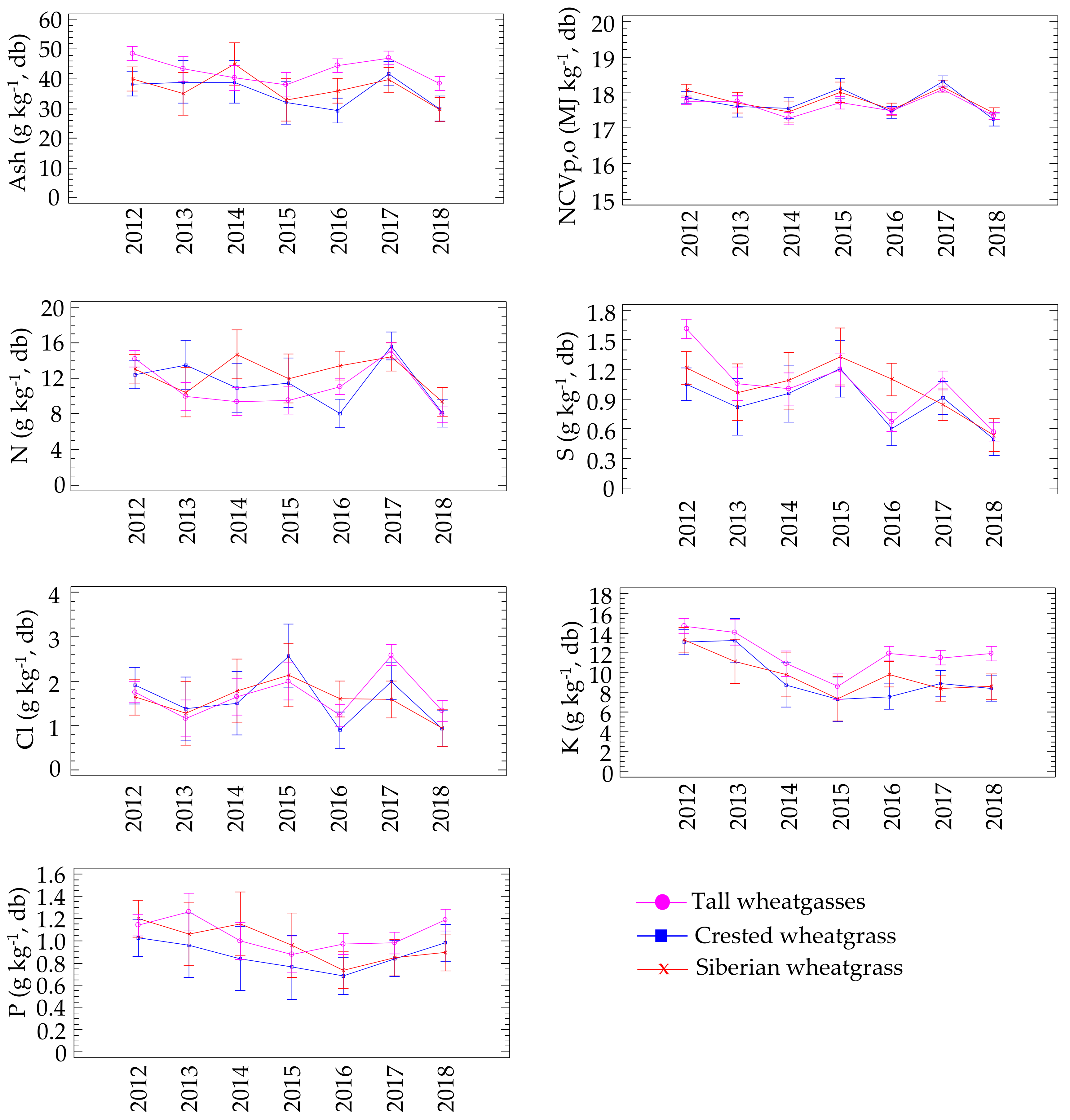
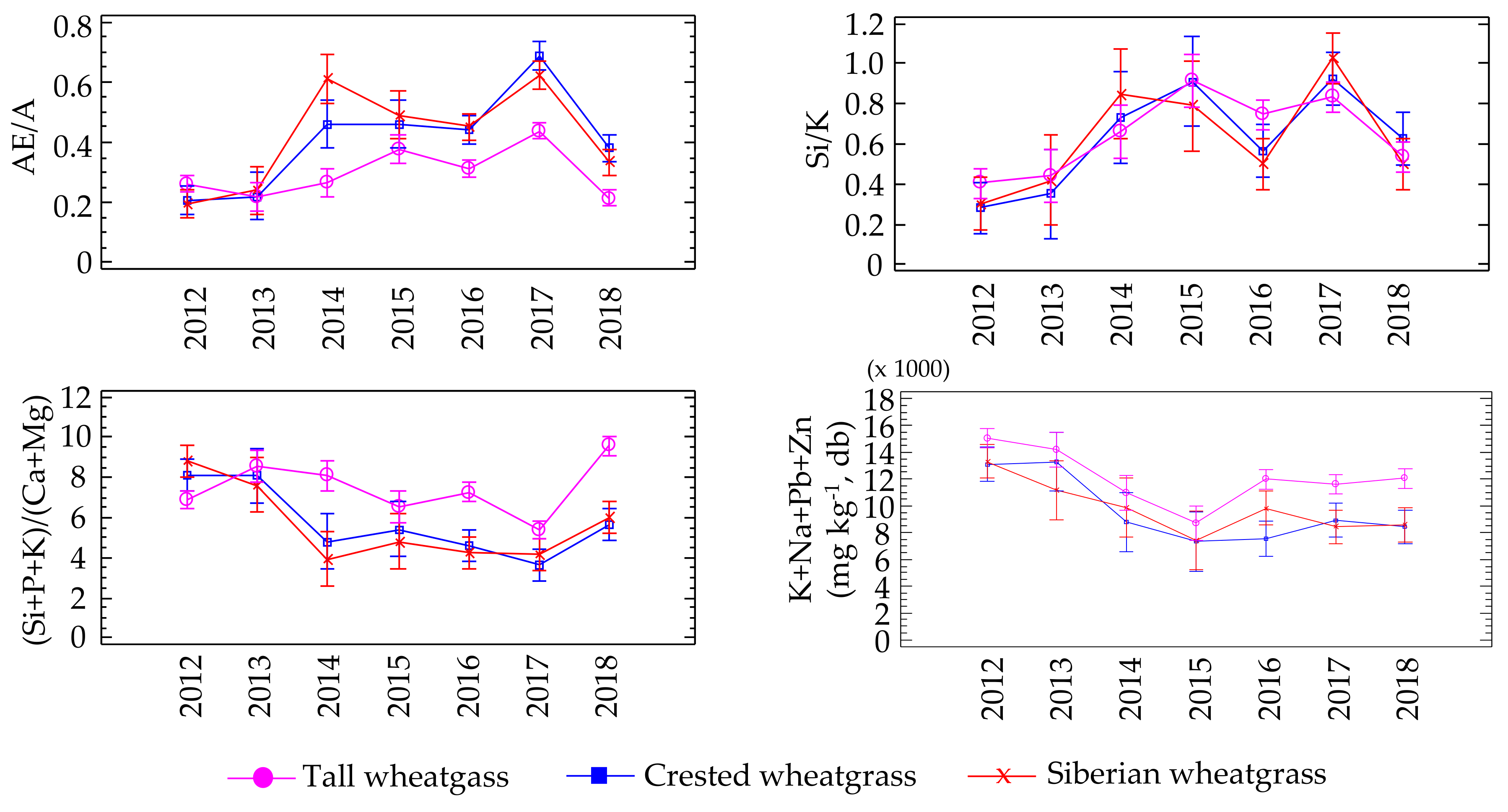
When grown in the same location (CS), the main differences were found across species rather than among cultivars. In this sense, the chemical composition of tall wheatgrass cultivars differed from crested and Siberian wheatgrass, finding higher ash, K, Na, and Si contents for the former, which resulted in lower AE/A ratios and higher K/(Ca + Mg), (Si + P + K)/(Ca + Mg), and K + Na + Pb + Zn indices. Therefore, fuel indices predict a slightly better combustion behavior of crested and Siberian wheatgrass with regard to ash sintering and aerosol emissions.
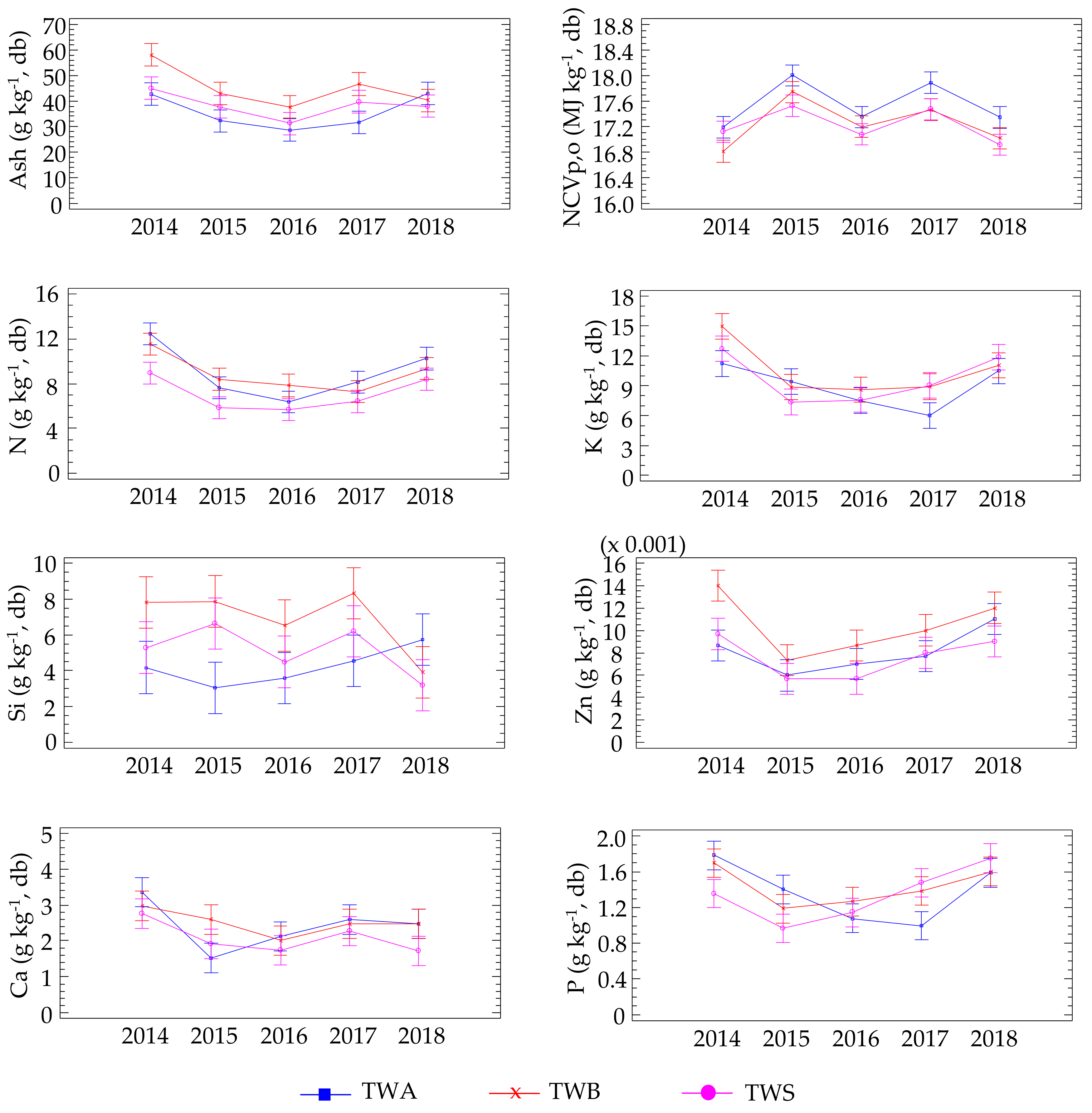
When different tall wheatgrass cultivars were grown in the same environment (TWA, TWJ, and TWR in CS and TWA, TWB, and TWS in AL), most of their properties varied in a relatively narrow range. Genotypic differences in the accumulation of minerals and the fuel quality of other grass species have been previously reported [30,45,71], and they can only be quantified when the grasses are grown at the same location.
However, it should be highlighted that the slight differences found among all the species and cultivars tested are not expected to be of any practical relevance if theses grasses are utilized in combustion processes. No matter the species or year considered, AE/A ratios were always maintained low (<0.8), and K/(Ca + Mg) ratios were >2, far from the guidelines to avoid sintering problems (AE/A >2 [52], and K/(Ca + Mg)<0.5 [53]). In addition, (Si + P + K)/(Ca + Mg) molar ratios were always from 3–10. Therefore, low sintering temperatures are expected for the cultivated grasses [52,53,54,55]. K + Na + Pb + Zn were always between 8000 and 16,000 mg kg−1 (Figure 5), suggesting medium aerosol emissions (PM1) for crested and Siberian wheatgrass to high aerosol emissions in the case of TW cultivars [54]. Si/K molar ratios were low (<1.2, Figure 5), also suggesting a high K release and aerosol formation.
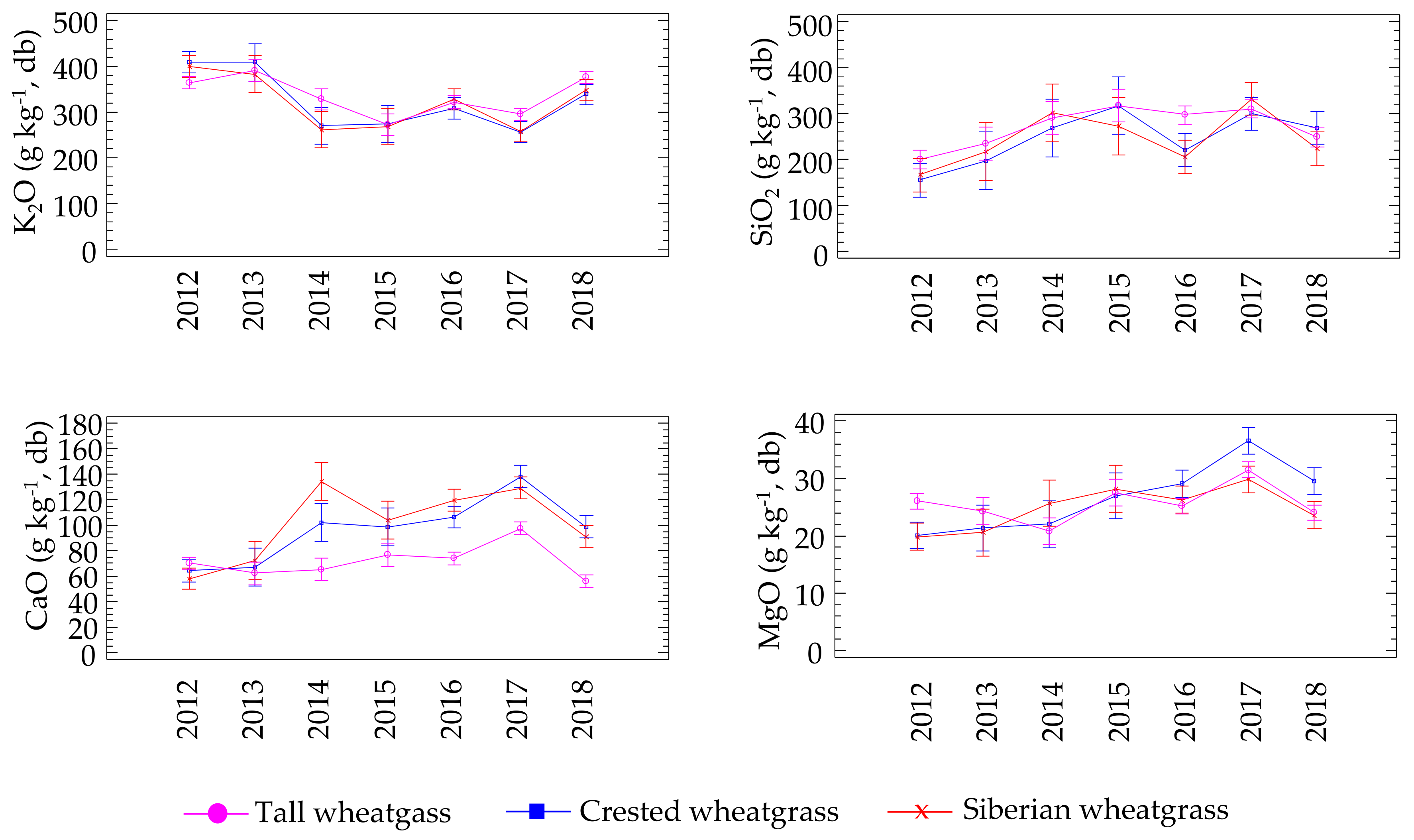
Our results suggest an improvement in the biomass quality of the grasses with crop age. In this sense, the ash content, as well as the concentrations of K, S, Na, and Cl, tended to decrease over the years, while the content of CaO, MgO, and SiO2 in the ashes tended to increase. As a result of the changes noted in the chemical composition, the biomass collected during the first years exhibited lower AE/A and Si/K ratios, and higher (Si + P + K)/(Ca + Mg) and K + Na + Pb + Zn indices. Therefore, the results obtained suggest a better ash fusibility behavior for the biomass harvested during the later years of the study, as well as lower gaseous and aerosol emissions. The positive effect of crop age on the chemical characteristics of other grasses was previously documented [31,42,45,56,71]. Similar to our results, ash content reductions and higher SiO2/K2O and CaO/K2O ratios were found in 10-year-old giant reed crops in central Italy [42]. The mineral concentration decline with plant maturation has been previously related to the different morphological characteristics of the stand crops during ageing, which produces a greater amount of thinner stems per unit area with fewer leaves [42,72]. However, as suggested by Di Nasso [42], it is very difficult to separate the effect of crop age from the effect of different annual meteorological conditions, particularly the rainfall distribution during the growing seasons.
Based on the chemical composition and the assessment of the calculated fuel combustion indices, the grasses cultivated in these marginal regions are expected to show the typical combustion behavior of cold perennial grasses harvested in summer. When assessing the fuel indices, results suggest that the differences found among wheatgrass species and cultivars for some of their combustion properties and chemical characteristics are not likely to affect their combustion behavior from a practical point of view. If these grasses are going to be used for producing bioenergy in a thermochemical conversion process, technological measures in power plants should be implemented to avoid sintering, corrosion, and emission-related problems [30,45,46]. Another possibility worth considering would be to try reducing the content of troublesome elements directly in the fuel. Practices, such as leaching during field drying or a harvest delay, have been proven effective for grasses [30,31,43,56,68,71], due to the reduction in ash content and water-soluble elements in the fuel, as well as an increase in ash deformation temperatures. The impact of leaching and/or a delayed harvest on the chemical composition and fuel quality parameters of theses grasses should be explored in marginal land and semi-arid environments with scarce precipitation and variable rain distribution. In addition, an economic assessment would also be useful to determine whether these alternatives would be viable in low-productive soils, as the improvement in the quality properties of the fuel is usually accompanied by significant dry matter losses and the risk of displacing the baling to periods with unfavorable weather conditions [43,71]. The biomass cultivated in this study could also be used to produce herbaceous pellets, class B [73]. The limitations established in ISO 17225-6 for herbaceous pellets, class A, would not be met, as the Cl content of the cultivated perennial grasses surpassed the limitation of 1.0 g·kg−1 db at both locations, but especially in AL, where higher levels of Na and Cl were found.

5. Conclusions

Tall wheatgrass can be an effective alternative for growing energy feedstock under marginal conditions as it provided better biomass yields and rain use efficiencies than crested and Siberian wheatgrass. Among all the tall wheatgrass cultivars tested, both Alkar and Szarvasi-1 provided the best biomass production. Agropyron spp. can achieve positive biomass yields in areas with biophysical constraints under rainfed conditions as long as the precipitation between March and June is higher than 150 mm.
The major differences in biomass composition were across species rather than among cultivars. Tall wheatgrass exhibited the highest ash content, K, Na, and Si concentrations. The net calorific value was higher in crested, Siberian, and tall wheatgrass cv. Riparianslopes than the rest of the tall wheatgrass cultivars. All species and cultivars showed similar fuel indices, being slightly better for crested and Siberian wheatgrass. In this sense, the differences found among species and cultivars regarding their main properties and chemical composition are not likely to be of any practical relevance if these grasses are utilized in combustion processes. The ash content, as well as the concentrations of K, S, Na, and Cl, tended to decrease over the years, while the content of other ash-forming elements, such as Ca, Mg, and Si, tended to increase, making the biomass collected during later years better in quality.
A genetic improvement of these grasses could be helpful to improve biomass productions for bioenergy in low-input agriculture. Later harvest times under marginal conditions should also be explored in order to improve the combustion quality of this type of biofuels.
This experiment could be replicated in more than 10 million ha located in Europe that have been categorized as marginal land [13], and where Agropyron spp., tall wheatgrass in particular, could perform well in terms of biomass production and water use efficiency. In addition, and according to FAOSTAT [74], there are more than five million hectares around the world that are actually sown with rye (Secale cereale L.), offering a doubtful positive economic margin and environmental balance [16], and which could be used to cultivate Agropyron species for bioenergy purposes. Further research should be carried out to assess whether later harvest dates, with the aim of improving the quality of the biomass produced, would be feasible under marginal conditions. Additionally, an assessment on the applicability of these grasses as feedstock for second-generation biofuels would be useful.

Author Contributions

Conceptualization, C.S.C. and R.B.; methodology, C.S.C, R.B. and M.S.; software, C.S.C., R.B. and M.S.; validation, C.S.C., R.B., M.S. and P.C.; formal analysis, C.S.C., R.B. and M.S.; investigation, C.S.C., R.B., M.S. and P.C.; resources, P.C.; data curation, C.S.C., R.B., M.S. and P.C.; writing—Original draft preparation, C.S.C.; writing—Review and editing, C.S.C., R.B., M.S. and P.C.; visualization, C.S.C., R.B., M.S. and P.C. supervision, R.B., M.S. and P.C.; project administration, P.C., funding acquisition, P.C. All authors have read and agreed to the published version of the manuscript.

Funding

This research received funding from the European Union’s Horizon 2020 research and innovation program under grant agreement No 727698. The article processing charge was funded by the European Union’s Horizon 2020 research and innovation program under grant agreement No 727698.

Acknowledgments

The authors would like to thank Javier Perez, Rocio Cortes and Emiliano Maletta for their valuable contribution to this work.

Conflicts of Interest

The authors declare that there is no conflict of interest.

References

  1. Rajagopal, D.; Sexton, S.E.; Roland-Holst, D.; Zilberman, D. Challenge of biofuel: Filling the tank without emptying the stomach? Environ. Res. Lett. 2007, 2, 1–9. [Google Scholar] [CrossRef]
  2. Mantineo, D.; D’Angosta, G.M.; Copani, V.; Patance, C.; Cosentino, S.L. Biomass yield and energy balance of three perennial crops for energy use in the semi-arid Mediterranean environment. Field Crop Res. 2009, 114, 204–213. [Google Scholar] [CrossRef]
  3. Nalepa, R.A.; Bauer, D.M. Marginal lands: The role of remote sensing in constructing landscapes for agrofuel development. J. Peasant Stud. 2012, 39, 403–422. [Google Scholar] [CrossRef]
  4. Dominguez Faus, R.; Powers, S.E.; Burken, J.G.; Alvarez, P.J. The water footprint of biofuels: A drink or drive issue? Environ. Sci. Technol. 2009, 43, 3005–3010. [Google Scholar] [CrossRef] [Green Version]
  5. Dauber, J.; Miyake, S. To integrate or to segregate food crop and energy crop cultivation at the landscape scale? Perspectives on biodiversity conservation in agriculture in Europe. Energy Sustain. Soc. 2016, 6, 25. [Google Scholar] [CrossRef] [Green Version]
  6. Mehmood, M.A.; Ibrahim, M.; Rashid, U.; Nawaz, M.; Ali, S.; Hussain, A.; Gull, M. Biomass production for bioenergy using marginal lands. Sustain. Prod. Consum. 2017, 9, 3–21. [Google Scholar] [CrossRef]
  7. Gerwin, W.; Repmann, F.; Spyridon, G.; Despoina, V.; Gounairs, N.; Baumgarten, W.; Christianes, V.; Keramitzis, D.; Kiourtsis, F.; Freese, D. Assessment and quantification of marginal lands for biomass production in Europe using soil quality indicators. Soil 2018, 4, 267–290. [Google Scholar] [CrossRef] [Green Version]
  8. Bordonal, R.d.O.; Nunes, J.L.; Lal, R.; de Figueiredo, E.B.; de Oliveira, B.G.; La Scala, N.J. Sustainability of sugarcane production in Brazil. A review. Agron. Sustain Dev. 2018, 38, 13. [Google Scholar] [CrossRef] [Green Version]
  9. Peterson, G.M.; Galbraith, J.K. The concept of marginal land. J. Farm Econ. 1932, 14, 295–310. [Google Scholar] [CrossRef]
  10. Liu, T.T.; McConkey, B.G.; Ma, Z.Y.; Liu, Z.G.; Li, X.; Cheng, L.L. Strengths, weaknesses, opportunities and threats analysis of bioenergy production on marginal land. Energy Procedia 2011, 5, 2378–2386. [Google Scholar] [CrossRef] [Green Version]
  11. Yakubu, A.S.; Ehlers, M.H.; Harnmeijer, J. Anaerobic digestion of feedstock grown on marginal land: Break-even electricity prices. Energies 2017, 10, 21. [Google Scholar]
  12. Shortall, O.K. “Marginal land” for energy crops. Exploring definitions and embedded assumtions. Energy Policy 2013, 62, 19–27. [Google Scholar] [CrossRef]
  13. Von Cossel, M.; Lewandowski, I.; Elbersen, B.; Staritsky, I.; Van Eupen, M.; Iqbal, Y.; Mantel, S.; Scordia, D.; Testa, G.; Cosentino, S.L.; et al. Marginal agricultural land low-input systems for biomass production. Energies 2019, 12, 25. [Google Scholar] [CrossRef] [Green Version]
  14. Ruf, T.; Audu, V.; Holzhauser, K.; Emmerling, C. Bioenergy from periodically waterlogged cropland in Europe: A first assessment of the potential of five perennial energy crops to provide biomass and their interactions with soil. Agronomy 2019, 9, 25. [Google Scholar] [CrossRef] [Green Version]
  15. Acharya, B.S.; Blanco-Canqui, H. Lignocellulosic-based bioenergy and water quality parameters: A review. Glob. Change Biol. Bioenergy 2018, 10, 504–533. [Google Scholar] [CrossRef] [Green Version]
  16. Ciria, C.S.; Sastre, C.M.; Carrasco, J.; Ciria, P. Tall wheatgrass (Thinopyrum ponticum (Podp.)) in a real farm context, a sustainable perennial alternative to rye (Secale cereale L.) cultivation in marginal lands. Ind. Crop. Prod. 2020, 146, 8. [Google Scholar] [CrossRef] [Green Version]
  17. Blanco-Canqui, H. Energy crops and their implications on soil and environment. Agron. J. 2010, 102, 403–419. [Google Scholar] [CrossRef]
  18. Chimento, C.; Almagro, M.; Amaducci, S. Carbon sequestration potential in perennial bioenergy crops: The importance of organic matter inputs and its physical protection. Glob. Change Biol. Bioenergy 2016, 8, 111–121. [Google Scholar] [CrossRef]
  19. Haughton, A.J.; Bohan, D.A.; Clark, S.J.; Mallot, M.D.; Mallot, V.; Sage, R.; Karp, A. Dedicated biomass crops can enhance biodiversity in the arable landscape. Glob. Change Biol. Bioenergy 2016, 8, 1071–1081. [Google Scholar] [CrossRef] [PubMed] [Green Version]
  20. Fernando, A.L.; Boleó, S.; Barbosa, B.; Costa, J.; Duarte, M.P.; Monti, A. Perennial grass production opportunities on marginal Mediterranean land. Bioenergy Res. 2015, 8, 1523–1537. [Google Scholar] [CrossRef]
  21. Landis, D.A.; Gratton, C.; Jackson, R.D.; Gross, K.L.; Duncan, D.S.; Liang, C.; Meehan, T.D.; Robertson, B.A.; Schmidt, T.M.; Stahlheber, K.A.; et al. Biomass and biofuel crop effects on biodiversity and ecosystem services in the North Central US. Biomass Bioenergy 2018, 114, 18–29. [Google Scholar] [CrossRef]
  22. Ruf, T.; Makselon, J.; Udelhoven, T.; Emmerling, C. Soil quality indicator response to land-use change from annual to perennial bioenergy cropping systems in Germany. Glob. Change Biol. Bioenergy 2018, 10, 444–459. [Google Scholar] [CrossRef]
  23. Dickeduisberg, M.; Laser, H.; Tonn, B.; Isselstein, J. Tall wheatgrass (Agropyron elongatum) for biogas production: Crop management more important for biomass and methane yield than grass provenance. Ind. Crop. Prod. 2017, 97, 653–663. [Google Scholar] [CrossRef]
  24. Tufekcioglu, A.; Raich, J.W.; Isenhart, T.M.; Schultz, R.C. Biomass, carbon and nitrogen dynamics of multi-species riparian buffers within an agricultural watershed in Iowa, USA. Agrofor. Syst. 2003, 57, 187–198. [Google Scholar] [CrossRef]
  25. Glover, J.D.; Culman, S.W.; DuPont, S.T.; Broussard, W.; Young, L.; Mangan, M.E.; Mai, J.G.; Crews, T.E.; DeHaan, L.R.; Buckley, D.H.; et al. Harvested perennial grasslands provide ecological benchmarks for agricultural sustainability. Agr. Ecosyst. Environ. 2010, 137, 3–12. [Google Scholar] [CrossRef]
  26. Pulighe, G.; Bonati, G.; Fabiani, S.; Barsali, T.; Lupia, F.; Vanino, S.; Nino, P.; Arca, P.; Roggero, P.P. Assessment of the agronomic feasibility of bioenergy crop cultivation on marginal and polluted land: A GIS-based. Suitability study from Sulcis area, Italy. Energies 2016, 9, 19. [Google Scholar] [CrossRef]
  27. Jiang, W.; Jacobson, M.G.; Langholtz, M.H. A sustainability framework for assessing studies about marginal lands for planting perennial energy crops. Biofuel Bioprod. Bior. 2019, 13, 228–240. [Google Scholar] [CrossRef] [Green Version]
  28. Podlaski, S.; Pietkiewicz, S.; Choluj, D.; Horaczek, T.; Wisniewski, G.; Gozdowski, D.; Kalaji, H.M. The relationship between the soil water storage and water-use efficiency of seven energy crops. Photosynthetica 2017, 55, 210–218. [Google Scholar] [CrossRef] [Green Version]
  29. Agostini, F.; Gregory, A.S.; Richter, G.M. Carbon sequestration by perennial energy crops: Is the jury still out? Bioenergy Res. 2015, 8, 1057–1080. [Google Scholar] [CrossRef] [Green Version]
  30. Lewandowski, I.; Scurlock, J.M.O.; Lindwall, E.; Christou, M. The development and current status of perennial rhizomatous grasses as energy crops in the US and Europe. Biomass Bioenergy 2003, 25, 335–361. [Google Scholar] [CrossRef]
  31. Nazli, R.I.; Tansi, V.; Ozturk, H.H.; Kusvuran, A. Miscanthus, switchgrass, giant reed, and bulbous canary grass as potential bioenergy crops in a semi-arid Mediterranean environment. Ind. Crop. Prod. 2018, 125, 9–23. [Google Scholar] [CrossRef]
  32. Cherney, J.H.; Johnson, K.D.; Lechtenberg, V.L.; Hertel, J.M. Biomass yield, fiber composition and persistence of cool season grasses. Agric. Biomass 1986, 10, 175–186. [Google Scholar] [CrossRef]
  33. Shan, C.J.; Liang, Z.S. Jasmonic acid regulates ascorbate and glutathione metabolism in Agropyron cristatum leaves under water stress. Plant Sci. 2010, 178, 130–139. [Google Scholar] [CrossRef]
  34. Wu, J.; Yang, X.M.; Wang, H.; Li, H.J.; Li, L.H.; Li, X.Q.; Liu, W.H. The introgression of chromosome 6P specifying for increased numbers of florets and kernels from Agropyron cristatum into wheat. Theor. Appl. Genet. 2006, 114, 13–20. [Google Scholar] [CrossRef] [PubMed]
  35. Himmel, M.E.; Ding, S.Y.; Johnson, D.K.; Adney, W.S.; Nimlos, M.R.; Brady, J.W.; Foust, T.D. Biomass recalcitrance: Engineering plants and enzymes for biofuels production. Science 2007, 315, 804–807. [Google Scholar] [CrossRef] [PubMed] [Green Version]
  36. Jafari, A.A.; Elmi, A.; Bakhtiari, M. Evaluation of yield and quality traits in 17 population of tall wheatgrass (Agropyron elongatum) grown in a rainfed area of Iran, under two cutting management. Rom. Agric. Res. 2014, 31, 792–797. [Google Scholar]
  37. Lauriault, L.M.; Kirksey, R.E.; Donart, G.B. Irrigation and nitrogen effects on tall wheatgrass yield in the Southern High Plains. Agron. J. 2002, 94, 792–797. [Google Scholar] [CrossRef]
  38. Jasinskas, A.; Zaltauskas, A.; Kryzeuiciene, A. The investigation of growing and using of tall perennial grasses as energy crops. Biomass Bioenergy 2008, 32, 981–987. [Google Scholar] [CrossRef]
  39. Monono, E.M.; Nyren, R.E.; Berti, M.T.; Pryor, S.W. Variability in biomass yield, chemical composition, and ethanol potential of individual and mixed herbaceous biomass species grown in North Dakota. Ind. Crop. Prod. 2013, 41, 331–339. [Google Scholar] [CrossRef]
  40. Jefferson, P.G.; McCaughey, W.P.; May, K.; Woosaree, J.; McFarlane, L. Potential utilization of native prairie grasses from western Canada as ethanol feedstock. Can. J. Plant Sci. 2004, 84, 1067–1075. [Google Scholar] [CrossRef]
  41. Martyniak, D.; Zurek, G.; Prokopiuk, K. Biomass yield and quality of wild populations of tall wheatgrass Elymus elongatus (Host.) Runemark. Biomass Bioenergy 2017, 101, 21–29. [Google Scholar] [CrossRef]
  42. Di Nasso, N.N.O.; Angelini, L.G.; Bonari, E. Influence of fertilisation and harvest time on fuel quality of giant reed (Arundo donax L.) in central Italy. Eur. J. Agron. 2010, 32, 219–227. [Google Scholar] [CrossRef]
  43. Prochnow, A.; Heiermann, M.; Ploechl, M.; Linke, B.; Idler, C.; Amon, T.; Hobbs, P.J. Bioenergy from permanent grassland—A review: 1. Biogas. Bioresour. Techol. 2009, 100, 4931–4944. [Google Scholar] [CrossRef] [PubMed]
  44. Florine, S.E.; Moore, K.J.; Fales, S.L.; White, T.A.; Burras, C.L. Yield and composition of herbaceous biomass harvested from naturalized grassland in southern Iowa. Biomass Bioenergy 2006, 30, 522–528. [Google Scholar] [CrossRef]
  45. El Nashaar, H.M.; Griffith, S.M.; Steiner, J.J.; Banowetz, G.M. Mineral concentration in selected native temperate grasses with potential use as biofuel feedstock. Bioresour. Technol. 2009, 100, 3526–3531. [Google Scholar] [CrossRef] [PubMed]
  46. Obernberger, I.; Brunner, T.; Baernthaler, G. Chemical properties of solid biofuels—significance and impact. Biomass Bioerg. 2006, 30, 973–982. [Google Scholar] [CrossRef]
  47. Ciria, C.S.; Sanz, M.; Carrasco, J.; Ciria, P. Identification of arable marginal lands under rainfed conditions for bioenergy purposes in Spain. Sustainability 2019, 11, 17. [Google Scholar] [CrossRef] [Green Version]
  48. Dardel, C.; Kergoat, L.; Hiernaux, P.; Grippa, M.; Mougin, E.; Ciais, P.; Nguyen, C. Rain-Use-Efficiency: What it tells us about the conflicting Sahel greening and Sahelian paradox. Remote Sens. 2014, 6, 3446–3474. [Google Scholar] [CrossRef] [Green Version]
  49. Hendrickson, J.R.; Schmer, M.R.; Sanderson, M.A. Water use efficency by switchgrass compared to a native grass or a native grass alfalfa mixture. Bioenergy Res. 2013, 6, 746–754. [Google Scholar] [CrossRef] [Green Version]
  50. Frank, A.B.; Bauer, A. Rooting activity and water-use during vegetative development of crested and western wheatgrass. Agron. J. 1991, 83, 906–910. [Google Scholar] [CrossRef]
  51. ISO 14780:2017 Solid Biofuels—Sample Preparation. Available online: https://www.iso.org/standard/66480.html (accessed on 4 April 2020).
  52. Llorente, M.J.; Carrasco, J.E. Comparing methods for predicting the sintering of biomass ash in combustion. Fuel 2005, 84, 1893–1900. [Google Scholar] [CrossRef]
  53. Johnson, J.M.F.; Gresham, G.L. Do yield and quality of big bluestem and switchgrass feedstock decline over winter? Bioenergy Res. 2014, 7, 68–77. [Google Scholar] [CrossRef]
  54. Sommersacher, P.; Brunner, T.; Obernberger, I. Fuel indexes: A novel method for the evaluation of relevant combustion properties of new biomass fuels. Energy Fuel 2012, 26, 380–390. [Google Scholar] [CrossRef]
  55. Zeng, T.; Weller, N.; Pollex, A.; Lenz, V. Blended biomass pellets as fuel for small scale combustion appliances: Influence on gaseous and total particulate matter emissions and applicability of fuel indices. Fuel 2016, 184, 689–700. [Google Scholar] [CrossRef]
  56. Nazli, R.I.; Tansi, V. Influences of nitrogen fertilization and harvest time on combustion quality of four perennial grasses in a semi-arid Mediterranean climate. Ind. Crop. Prod. 2019, 128, 239–247. [Google Scholar] [CrossRef]
  57. Boehmel, C.; Lewandowski, I.; Claupein, W. Comparing annual and perennial energy cropping systems with different management intensities. Agric. Syst. 2008, 96, 224–236. [Google Scholar] [CrossRef]
  58. Pearson, C.H.; Larson, S.R.; Keske, C.M.H.; Jensen, K.B. Native grasses for biomass production at high elevation, in Industrial crops. In Handbook of Plant Breeding, 1st ed.; Cruz, V.M.V., Dierig, D.A., Eds.; Springer: New York, NY, USA, 2014; Volume 9, pp. 101–132. [Google Scholar]
  59. Wang, G.J.; Nyren, P.; Xue, Q.W.; Aberle, E.; Eriksmoen, E.; Tjelde, T.; Liebig, M.; Nichols, K.; Nyren, A. Establishment and Yield of Perennial Grass Monocultures and Binary Mixtures for Bioenergy in North Dakota. Agron. J. 2014, 106, 1605–1613. [Google Scholar] [CrossRef]
  60. Pedroso, G.M.; Hutmacher, R.B.; Putnam, D.; Six, J.; Van Kessel, C.; Linquist, B.A. Biomass yield and nitrogen use of potential C-4 and C-3 dedicated energy crops in a Mediterranean climate. Field Crops Res. 2014, 161, 149–157. [Google Scholar] [CrossRef]
  61. Suyama, H.; Benes, S.E.; Robinson, P.H.; Getachew, G.; Grattan, S.R.; Grieve, C.M. Biomass yield and nutritional quality of forage species under long-term irrigation with saline-sodic drainage water: Field evaluation. Anim. Feed Sci. Tech. 2007, 135, 329–345. [Google Scholar] [CrossRef]
  62. Sandor, C. Tall wheatgrass cultivar Szarvasi-1 (Elymus elongatus subsp. ponticus cv. Szarvasi-1) as a potential energy crop for semi-arid lands of eastern Europe. In Sustainable Growth and Applications in Renewable Energy Sources, 1st ed.; Nayeripour, M., Ed.; Intech Open: Pécs, Hungary, 2011; pp. 269–294. [Google Scholar]
  63. Danielewicz, D.; Surma-Slusarska, B.; Zurek, G.; Martyniak, D. Selected grass plants as biomass fuels and raw materials for papermaking. Part I. Calorific value and chemical composition. Bioresources 2015, 10, 8539–8551. [Google Scholar] [CrossRef] [Green Version]
  64. Jensen, K.B.; Johnson, D.A.; Asay, K.H.; Olson, K.C. Seasonal-accumulated growth and forage quality of range grasses for fall and winter grazing. Can. J. Plant Sci. 2002, 82, 329–336. [Google Scholar] [CrossRef] [Green Version]
  65. Johnson, D.A.; Asay, K.H.; Jensen, K.B. Carbon isotope discrimination and yield in 14 cool-season grasses. J. Range Manag. 2003, 56, 654–659. [Google Scholar] [CrossRef]
  66. Cable, D.R. Influence of precipitation on perennial grass production in semidesert southwest. Ecology 1975, 56, 981–986. [Google Scholar] [CrossRef]
  67. Tello-Garcia, E.; Huber, L.; Leitinger, G.; Peters, A.; Newesely, C.; Ringler, M.E.; Tasser, E. Drought- and heat-induced shifts in vegetation composition impact biomass production and water use of alpine grasslands. Environ. Exp. Bot. 2020, 169, 10. [Google Scholar] [CrossRef]
  68. ISO 17225-1:2014 Solid Biofuels–Fuel Specifications and Classes—Part 1: General requirements. Available online: https://www.iso.org/standard/59456.html (accessed on 4 April 2020).
  69. Shield, I.F.; Barraclough, T.J.P.; Riche, A.B.; Yates, N.E. The yield response of the energy crops switchgrass and reed canary grass to fertiliser applications when grown on a low productivity sandy soil. Biomass Bioenergy 2012, 42, 86–96. [Google Scholar] [CrossRef]
  70. Jenkins, B.M.; Bakker, R.R.; Wei, J.B. On the properties of washed straw. Biomass Bioenergy 1996, 10, 177–200. [Google Scholar] [CrossRef]
  71. Iqbal, Y.; Lewandowski, I. Inter-annual variation in biomass combustion quality traits over five years in fifteen Miscanthus genotypes in south Germany. Fuel Process. Technol. 2014, 121, 47–55. [Google Scholar] [CrossRef]
  72. Angelini, L.G.; Ceccarini, L.; Bonari, E. Biomass yield and energy balance of giant reed (Arundo donax L.) cropped in central Italy as related to different management practices. Eur. J. Agron. 2005, 22, 375–389. [Google Scholar] [CrossRef]
  73. ISO 17225-6:2014 Solid Biofuels—Fuel Specifications and Classes—Part 6: Graded Non Woody Pellets. Available online: https://www.iso.org/standard/59461.html (accessed on 7 April 2020).
  74. FAOSTAT, Food and Agriculture Data. Available online: http://www.fao.org/faostat/en/#data/QC (accessed on 15 February 2020).
Figure 1. Rainfall and temperature data for Cubo de la Solana fields during the study years. Hollow and filled bars indicate different consecutive years.
Agronomy 10 01051 g001
Figure 2. Rainfall and temperature data for Alconaba fields during the study period. Hollow and filled bars indicate different consecutive years.
Agronomy 10 01051 g002
Figure 3. Net calorific value, ash, N, P, K, S, and Cl contents across species and years for the biomass cultivated in CS fields. Means and Fisher´s LSD interaction plots.
Agronomy 10 01051 g003
Figure 4. Si, K, Ca, and Mg variation across species and years for the biomass cultivated in CS fields (concentrations expressed as their corresponding oxides in the ash). Means and Fisher’s LSD interaction plots.
Agronomy 10 01051 g004
Figure 5. Net calorific value, ash, N, P, K, Ca, Si, and Zn contents across cultivars and years for the biomass cultivated in AL fields. Means and Fisher´s LSD interaction plots.
Agronomy 10 01051 g005
Figure 6. Fuel indices across species and years for the biomass cultivated in the CS fields. Means and Fisher´s LSD interaction plots.
Agronomy 10 01051 g006
Table 1. Analytical techniques and standards followed during testing.
PropertyAnalytical Technique (Equipment)Standard
Sample preparationSubsampling and millingISO 14780:2017
AshCalcination at 550 °CISO 18122:2015
C, H, NElemental analysis by IRD and TCD (TruSpec, Leco)ISO 16948:2015
S and ClCombustion bomb + IC (883 Basic IC Plus, Metrohm)ISO 16994:2016
Calorific valueCalorimetry (C5003, Ika Verke)ISO 18125:2017
Major elements: Al, Ca, Fe, K, Mg, Mn, Na, P, Si, Ti, ZnMW digestion (Ethos Pro, Milestone) + ICP-OES (Jarrell Ash, Thermo Fisher)ISO 16967:2015
IRD: Infrared Detection; TCD: Thermal Conductivity Detection, IC: Ion Chromatography; MW: microwave digestion; ICP-OES: Inductively Coupled Plasma—Optical Emission Spectroscopy.
Table 2. Variance analysis of the fixed effect of species (S), cultivars (C), and year (Y) on dry matter yields and RUE of the biomass produced.
YieldRUE
SourcedfF-Valuep-ValuedfF-Valuep-Value
CS fields
S24.510.013027.910.0006
Y745.610.0000728.560.0000
S × Y143.650.0001143.630.0001
AL fields
C22.700.035725.170.0087
Y49.380.000043.530.0124
C × Y83.980.001286.450.0000
df: degrees of freedom.
Table 3. Biomass yields from CS and AL stations. Data provided in Mg of dry matter (DM)·ha−1.
FieldsS/CYears
20112012201320142015201620172018Mean
CSTWA2.02.67.53.35.35.90.111.54.8 ± 3.6 a
TWJ2.02.67.62.84.05.90.212.64.7 ± 3.9 a
TWR2.02.17.13.34.65.80.211.54.6 ± 3.6 a,b
CWR1.22.65.71.72.81.90.36.52.8 ± 2.2 b
SWV1.32.26.31.92.92.10.36.72.9 ± 2.3 a,b
mean± SD1.7 ± 0.4 d2.4 ± 0.2 d6.9 ± 0.8 b2.6 ± 0.8 d3.9 ± 1.1 c4.3 ± 2.1 c0.2 ± 0.1 e9.8 ± 2.9 a
ALTWB---1.34.73.93.24.43.5 ± 1.5 a,b
TWS---3.57.03.72.35.14.3 ± 1.8 a
TWA- -0.92.53.72.85.23.0 ± 1.3 b
mean± SD---1.9 ± 1.4 c4.7 ± 2.2 a3.8 ± 0.1 ab2.8 ± 0.4 b,c4.9 ± 0.4 a
S: species; C: cultivar; SD: standard deviation. Different letters indicate significant different means between cultivars and years for that property at the 95% confidence level according to multiple range tests.
Table 4. RUE from CS and AL stations. Data provided in g DM·L−1.
FieldsS/CYears
20112012201320142015201620172018Mean
CSTWA0.91.92.92.12.22.80.12.82.0 ± 1.0 a
TWJ1.01.92.91.81.62.80.23.11.9 ± 1.0 a
TWR1.01.52.82.11.92.70.22.81.9 ± 0.9 a
CWR0.61.92.21.11.20.90.21.61.2 ± 0.7 b
SWV0.61.62.41.21.21.00.21.61.2 ± 0.7 b
mean± SD0.8 ± 0.2 d1.8 ± 0.2 c2.6 ± 0.3 a1.6 ± 0.5 c1.6 ± 0.4 c2.0 ± 1.0 b c0.2 ± 0.1 e2.4 ± 0.7 a,b
ALTWB---1.02.42.01.81.41.8 ± 0.5 a,b
TWS---2.73.62.01.11.72.2 ± 0.9 a
TWA- -0.71.32.01.31.71.4 ± 0.5 b
mean± SD---1.5 ± 1.1 b2.4 ± 1.1 a2.0 ± 0.1 a,b1.4 ± 0.4 b1.6 0.1 b
S: species; C: cultivar; SD: standard deviation. Different letters indicate significant different means between cultivars and years for that property at the 95% confidence level according to multiple range tests.
Table 5. Influence of the different species, cultivars, and years on the biomass properties and chemical composition of the biomass cultivated at two locations (CS and AL).
CS BiomassAL Biomass
FactorS/CYS/C × YCYC × Y
df4624248
Ash****ns****ns
C***ns****ns
H****ns*ns*
Nns**ns****ns
Sns**ns****ns
Clns**ns******
GCVv,0****ns****ns
NCVp,0***ns****ns
Alns**nsns**ns
Cans***ns**ns
Fens**nsnsnsns
K****ns***ns
Mg***nsnsnsns
Mnns**nsns*ns
Na***nsnsnsns
Pns*nsns****
Si***ns**nsns
Zn**********ns
S: species; C: cultivar; Y: year; df: degrees of freedom; ** p-value < 0.01; * p-value = 0.01–0.05; ns: p-value > 0.05, according to Fisher´s tests (order 2 ANOVA).
Table 6. Ash content, calorific values, and ultimate analysis of the biomass of different perennial grasses collected between 2012 and 2018 at CS plots. Mean values for three replicate plots per species, cultivar, and year.
AshCHNSClGCVv,0NCVp,0
S/CY(g·kg−1 db)(g·kg−1 db)(g·kg−1 db)(g·kg−1 db)(g·kg−1 db)(g·kg−1 db)(MJ·kg−1 db)(MJ·kg−1 db)
TWA20124848260141.61.719.117.8
20134447360101.01.119.017.7
201445459609.51.01.718.617.3
20153947361111.31.919.217.9
20164347061120.71.118.517.2
20174748461150.92.019.117.8
201838472618.40.61.418.617.3
mean ±SD44 ± 4 a473 ± 8 b6.1 ± 0.5 b11 ± 2.41.0 ± 0.41.5 ± 0.418.9 ± 0.3 b17.6 ± 0.3 b
TWJ2012504806013.91.62.119.017.7
201345469609.61.11.418.817.5
201436458608.61.01.418.517.2
201537469618.51.21.919.017.6
2016444776110.90.81.218.817.5
2017484826314.91.33.219.618.3
201841475617.70.71.418.717.3
mean ±SD43 ± 5 a473 ± 8 b61 ± 1.0 b11 ± 31.1 ± 0.31.8 ± 0.718.9 ± 0.3 b17.6 ± 0.3 b
TWR2012484826014.51.61.519.217.9
2013414726010.01.01.019.418.1
2014404586010.11.01.818.617.3
201538456629.51.22.119.017.7
201646476619.90.51.419.117.8
2017464846316.11.12.519.618.2
201837472617.80.51.218.717.4
mean ±SD42 ± 4 b471 ± 11 b61 ± 1.0 b11.1 ± 3.01.0 ± 0.41.6 ± 0.519.1 ± 0.4 a17.8 ± 0.4 a
CWH2012384876112.41.11.919.217.9
2013394626113.50.81.418.917.6
2014394606110.91.01.518.917.6
2015324756211.51.22.619.518.1
2016294656308.10.60.918.917.5
2017424866315.60.92.019.718.3
2018304746208.10.50.918.617.2
mean ±SD36 ± 5 b473 ± 11 b62 ± 1.0 a11.4 ± 2.80.9 ± 0.21.6 ± 0.619.1 ± 0.4 a17.7 ± 0.4 a
SWV20124048861.313.11.21.619.418.1
20133.547561.010.41.01.319.017.7
20144546061.014.71.11.818.817.5
20153348161.012.01.32.119.418.0
20163647562.313.41.11.618.917.5
20174048763.014.40.81.619.518.2
20183047962.009.40.51.018.817.4
mean ±SD3.7 ± 0.5 b478 ± 9.0 a61.7 ± 0.8 a12.5 ± 2.01.0 ± 0.31.6 ± 0.419.1 ± 0.3 a17.8 ± 0.3 a
Global mean ±SD41 ± 7476 ± 961 ± 1.011.7 ± 3.11.0 ± 0.41.6 ± 0.719.0 ± 0.417.7 ± 0.4
Min. value27456606.20.40.818.316.9
Max. value584916418.91.94.619.818.5
P75464846214.01.21.919.317.9
Different letters indicate significant different means between species/cultivars for that property at the 95% confidence level according to multiple range tests. Letters were only included when the p-value for the cultivar factor was below 0.05.
Table 7. Major elements present in the biomass of different grasses collected at CS plots between 2012 and 2018. Mean values for three replicate plots per species and year.
AlCaFeKMgMnNaPSiZn
S/CY(g·kg−1 db)(g·kg−1 db)(g·kg−1 db)(g·kg−1 db)(g·kg−1 db)(g·kg−1 db)(g·kg−1 db)(g·kg−1 db)(g·kg−1 db)(g·kg−1 db)
TWA20120.092.30.03314.30.780.0690.351.14.30.012
20130.032.20.02513.80.700.0730.121.24.60.013
20140.052.10.00411.20.550.0790.061.06.80.013
20150.221.90.0988.60.610.0710.080.95.80.008
20160.062.30.02910.80.680.0670.071.06.90.008
20170.203.10.06211.00.850.1060.120.97.30.011
20180.041.60.01111.40.560.0520.221.24.90.011
mean ±SD0.10 ± 0.082.2 ± 0.40.037 ± 0.032 1.1.6 ± 1.9 a0.68 ± 0.11 a0.074 ± 0.0160.15 ± 0.10 a1.0 ± 0.15.8 ± 1.2 a0.011 ± 0.002 a
TWJ20120.142.50.04915.50.730.0950.211.34.30.013
20130.011.60.00814.50.580.0330.141.44.30.011
20140.041.60.01910.50.450.0850.051.04.00.012
20150.142.10.0838.40.610.0930.100.85.70.010
20160.082.60.04412.10.700.0930.071.05.60.011
20170.303.60.06611.80.920.1050.091.06.80.012
20180.051.40.02213.20.550.0890.021.34.60.017
mean ±SD0.11 ± 0.102.2 ± 0.80.042 ± 0.02712.3 ± 2.4 a0.65 ± 0.15 a,b0.085 ± 0.0240.10 ± 0.06 a1.1 ± 0.25.1 ± 1.0 a,b0.012 ± 0.002 a
TWR20120.092.50.03314.40.770.0760.341.14.30.012
20130.051.90.01914.00.620.0600.141.24.40.014
20140.031.90.00711.10.520.0700.051.04.70.013
20150.142.20.0718.70.670.0660.160.95.30.008
20160.042.20.02012.90.660.0790.071.06.00.011
20170.273.20.05511.70.900.0900.131.06.50.011
20180.061.60.03411.10.560.1110.121.14.30.0013
mean ±SD0.10 ± 0.082.2 ± 0.050.034 ± 0.02212.0 ± 2.0 a0.67 ± 0.13 a0.079 ± 0.0170.15 ± 0.10 a1.0 ± 0.15.1 ± 0.9 a,b0.012 ± 0.002 a
CWH20120.081.80.03313.10.470.0490.011.02.60.013
20130.021.90.01813.20.500.0630.041.03.40.018
20140.022.80.01008.70.520.1110.010.84.60.017
20150.132.30.06107.30.520.0640.030.84.80.010
20160.052.20.03207.50.520.080<0.010.73.00.010
20170.244.10.05408.90.920.2130.010.85.80.022
20180.052.10.01508.40.530.080<0.011.03.80.014
mean ±SD0.09 ± 0.082.5 ± 0.80.032 ± 0.0199.6 ± 2.5 b0.57 ± 0.16 b,c0.094 ± 0.0560.02 ± 0.01 b0.9 ± 0.14.0 ± 1.1 b0.015 ± 0.004 b
SWV20120.151.70.05113.30.480.0480.021.22.90.013
20130.021.80.01811.10.430.0430.021.13.30.011
20140.054.30.0269.80.700.1470.031.15.90.039
20150.162.50.0107.40.560.1070.041.04.20.012
20160.083.10.0439.80.570.1280.010.73.50.012
20170.223.70.0648.40.700.1910.010.86.30.016
20180.051.90.0118.60.420.080<0.010.93.10.014
mean0.10 ± 0.072.7 ± 1.00.045 ± 0.0269.8 ± 2.0 b0.55 ± 0.12c0.106 ± 0.0540.02 ± 0.01 b1.0 ± 0.24.2 ± 1.4 b0.017 ± 0.010 b
Global mean ±SD0.11 ± 0.082.4 ± 0.80.038 ± 0.02411.2 ± 2.60.64 ± 0.170.090 ± 0.050.09 ± 0.131.0 ± 0.24.8 ± 1.70.013 ± 0.005
Min. value0.011.1<0.0016.90.390.030<0.010.51.80.007
Max. value0.424.40.10018.41.020.2800.621.69.30.039
P750.142.80.05313.20.780.1000.121.25.90.014
Different letters indicate significant different means between species/cultivars for that property at the 95% confidence level according to multiple range tests. Letters were only included when the p-value for the cultivar factor was below 0.05.
Table 8. Ash content, calorific values, and ultimate analysis of the tall wheatgrass cultivars collected at AL plots from 2014–2018. Mean values for three replicate plots per cultivar and year.
AshCHNSClGCVv,0NCVp,0
CY(g·kg−1 db)(g·kg−1 db)(g·kg−1 db)(g·kg−1 db)(g·kg−1 db)(g·kg−1 db)(MJ·kg−1 db)(MJ·kg−1 db)
TWA2014434606212.41.42.418.517.2
201532478617.61.31.819.318.0
201629468616.40.71.418.717.4
201732481618.11.21.819.217.9
2018434806010.21.12.518.717.3
mean ±SD36 ± 7 b473 ± 9 a61.1 ± 0.7 a9.0 ± 2.4 a1.1 ± 0.3 a2.0 ± 0.5 b18.9 ± 0.4 a17.6 ± 0.4 a
TWB2014584526011.51.43.418.116.8
201543471618.41.23.919.117.7
201638460617.80.62.718.517.2
201747467607.31.05.218.817.5
201846464608.31.03.918.717.4
mean ±SD46 ± 7 a463 ± 7 b61 ± 0.4 b8.7 ± 1.6 a1.0 ± 0.3 a3.8 ± 0.9 a18.6 ± 0.4 b17.3 ± 0.4 b
TWS201445460619.01.15.318.517.1
201538468615.80.93.718.917.5
201631460625.70.51.318.417.1
201740470616.41.03.618.817.5
201836466616.00.82.918.717.4
mean ±SD38 ± 5 b464 ± 5 b61 ± 0.4 a6.6 ± 1.4 b0.9 ± 0.2 b3.3 ± 1.4 a18.6 ± 0.2 b17.3 ± 0.2 b
Global mean ±SD40 ± 8468 ± 1061.0 ± 0.78.3 ± 2.20.10 ± 0.030.28 ± 0.1518.7 ± 0.417.3 ± 0.4
Min. value2744859.05.10.050.0818.016.7
Max. value6348762.014.40.160.7119.418.1
P754647661.09.80.130.4019.017.6
Different letters indicate significant different means between cultivars for that property at the 95% confidence level according to multiple range tests. Letters were only included when the p-value for the cultivar factor was below 0.05.
Table 9. Major elements present in the biomass of the tall wheatgrass cultivars collected at AL plots from 2014-2018. Mean values for three replicate plots per cultivar and year.
AlCaFeKMgMnNaPSiZn
CY(g·kg−1 db)(g·kg−1 db)(g·kg−1 db)(g·kg−1 db)(g·kg−1 db)(g·kg−1 db)(g·kg−1 db)(g·kg−1 db)(g·kg−1 db)(g·kg−1 db)
TWA20140.163.40.07511.20.760.0310.311.84.20.009
20150.051.50.0219.40.500.0210.151.43.00.006
20160.132.10.1017.50.560.0280.171.13.60.007
20170.112.60.0416.00.660.0180.491.04.60.008
20180.092.50.13610.50.710.0240.421.65.70.011
mean ± SD0.11 ± 0.042.4 ± 0.70.075 ± 0.0468.9 ± 2.2 b0.64 ± 0.110.024 ± 0.0050.31 ± 0.151.4 ± 0.34.2 ± 1.0 b0.008 ± 0.002 b
TWB20140.123.00.04615.00.650.0320.411.77.80.014
20150.062.60.0208.90.590.0200.691.27.90.007
20160.082.00.0418.60.490.0200.331.36.50.008
20170.172.50.0308.90.560.0180.701.48.30.010
20180.122.70.0308.90.550.0190.571.38.60.009
mean ± SD0.11 ± 0.042.5 ± 0.350.034 ± 0.01010.1 ± 2.7 a0.57 ± 0.060.022 ± 0.010.54 ± 0.161.4 ± 0.207.8 ± 0.79 a0.010 ± 0.003 a
TWS20140.062.80.02712.70.560.0250.381.45.30.010
20150.061.90.0167.30.500.0160.541.06.60.006
20160.071.70.0517.60.500.0220.251.14.50.006
20170.142.30.0359.00.520.0140.401.56.20.008
20180.092.00.0348.00.510.0170.401.25.80.006
mean ± SD0.09 ± 0.032.1 ± 0.40.033 ± 0.0138.9 ± 2.2 b0.52 ± 0.020.019 ± 0.0050.40 ± 0.101.2 ± 0.25.7 ± 0.8 b0.007 ± 0.002 b
Global mean ± SD0.10 ± 0.062.3 ± 0.60.050 ± 0.0519.7 ± 2.60.59 ± 0.0140.025 ± 0.0150.36 ± 0.0291.4 ± 0.35.4 ± 2.20.009 ± 0.03
Min. value0.021.30.0145.50.380.0110.000.92.30.005
Max. value0.283.80.32716.81.140.1081.272.010.40.017
P750.132.80.05511.40.660.0280.541.67.10.010
Different letters indicate significant different means between cultivars for that property at the 95% confidence level according to multiple range tests. Letters were only included when the p-value for the cultivar factor was below 0.05.
Table 10. Empirical fuel predictive indices for the biomass cultivated at both locations (CS and AL) and significance levels for the factors considered. Values averaged across the years.
CS Biomass Speciesp-Values
Fuel indexUnitsTWCWSWSYS × Y
AE/A 0.30 b0.41 a0.42 a******
K/(Ca + Mg) 4.4 a3.5 b3.4 b******
(Si + P + K)/(Ca + Mg)molar ratio7.5 a5.8 b5.7 b******
K + Na + Pb + Znmg kg−1 db12100 a9600 b9800 b****ns
Si/Kmolar ratio0.65 a0.63 a0.63 ans**ns
2S/Clmolar ratio1.5 a1.3 a1.4 ans**ns
(K + Na)/4.9*(2S + Cl)molar ratio1.9 a1.5 a1.5 ans**ns
AL biomass Cultivarsp-values
Fuel indexUnitsTWATWBTWSCYC × Y
AE/A 0.47 a0.37 a,b0.34 b***
K/(Ca + Mg) 2.8 a3.1 a3.3 ans**
(Si + P + K)/(Ca + Mg)molar ratio5.1 b7.3 a6.9 a**nsns
K + Na + Pb + Znmg kg−1 db8400 b10700 a9500 a,b***ns
Si/Kmolar ratio0.75 a1.20 a0.91 ans**ns
2S/Clmolar ratio1.38 a0.60 b0.63 b**ns**
(K + Na)/4.9*(2S + Cl)molar ratio1.0 a0.6 a0.7 ans***
S: species; C: cultivar; Y: year; df: degrees of freedom; ** p-value < 0.01; * p-value = 0.01–0.05; ns: p-value > 0.05, according to Fisher´s tests (order 2 ANOVA). Different letters indicate significant different means between those species or cultivars for that index at the 95% confidence level according to multiple range tests.

