Base Neutralizing Capacity of Agricultural Soils in a Quaternary Landscape of North-East Germany and Its Relationship to Best Management Practices in Lime Requirement Determination

Abstract

Despite being a natural soil-forming process, soil acidification is a major agronomic challenge under humid climate conditions, as soil acidity influences several yield-relevant soil properties. It can be counterbalanced by the regular application of agricultural lime to maintain or re-establish soil fertility and to optimize plant growth and yield. To avoid underdose as well as overdose, lime rates need to be calculated carefully. The lime rate should be determined by the optimum soil pH (target pH) and the response of the soil to lime, which is described by the base neutralizing capacity (BNC). Several methods exist to determine the lime requirement (LR) to raise the soil pH to its optimum. They range from extremely time-consuming equilibration methods, which mimic the natural processes in the soil, to quick tests, which rely on some approximations and are designed to provide farmers with timely and cost-efficient data. Due to the higher analytical efforts, only limited information is available on the real BNC of particular soils. In the present paper, we report the BNC of 420 topsoil samples from Central Europe (north-east Germany), developed on sediments from the last ice age 10,000 years ago under Holocene conditions. These soils are predominantly sandy and low in humus, but they exhibit a huge spatial variability in soil properties on a small scale. The BNC was determined by adding various concentrations of Ca(OH)₂ and fitting an exponential model to derive a titration curve for each sample. The coefficients of the BNC titration curve were well correlated with soil properties affecting soil acidity and pH buffer capacity, i.e., pH, soil texture and soil organic matter (SOM). From the BNC model, the LRs (LR_BNC) were derived and compared with LR_VDLUFA based on the standard protocol in Germany as established by the Association of German Agricultural Analytic and Research Institutes (VDLUFA). The LR_BNC and LR_VDLUFA correlated well but the LR_VDLUFA were generally by approximately one order of magnitude higher. This is partly due to the VDLUFA concept to recommend a maintenance or conservation liming, even though the pH value is in the optimum range, to keep it there until the next lime application during the following rotation. Furthermore, the VDLUFA method was primarily developed from field experiments where natural soil acidification and management practices depressed the effect of lime treatment. The BNC method, on the other hand, is solely based on laboratory analysis with standardized soil samples. This indicates the demand for further research to develop a sound scientific algorithm that complements LR_BNC with realistic values of annual Ca²⁺ removal and acidification by natural processes and N fertilization.

1. Introduction

Soil acidity is a key factor in soil fertility, since it influences the availability of nutrients and toxic substances, as well as affects the aggregate stability and activity of soil biota, amongst others [1,2,3]. Soil acidity is defined as the sum of acids in a soil, which can neutralize bases by releasing protons [4]. Soil acidification is one of the most common agronomic challenges in leaching climates and highly productive areas [5]. It involves the leaching of cationic nutrients (e.g., Ca²⁺, K⁺ and Mg²⁺) and increases the availability of toxic Al cation species. As has been known for centuries, acidic soils can be ameliorated by the application of lime in order to improve crop production. Mainly via an increase in soil pH, liming influences a wide range of soil properties and processes that have positive effects on crop yield [6,7]. However, also high pH values above 7.5 can have adverse effects. Hence, lime rates have to be calculated carefully. Even though one can deduct from the soil pH value whether a soil is acidic or alkaline, the pH value alone does not provide sufficient information on the soil acidity. Soil pH reflects only the H⁺ concentration in the soil solution (active acidity) while the absorbed H⁺ and Al³⁺ cations represent the potential acidity, which in cultivated soils is much higher than the active acidity [8]. In the pH range from 4.5 to 7.5, the pH is mainly buffered by association/dissociation reactions of H⁺ ions while dissolution/precipitation processes are relatively slow [1].

For the adequate determination of lime requirements (LR), three pieces of information are required: the current state of the soil acidity, the soil’s response characteristics (buffering) to lime, and the optimum (target) pH value to be achieved. To quantify soil acidity, the pH buffering and lime requirement of soils, several techniques were developed which can be classified according to Sims [9] as follows:

• Soil–lime incubations:
  They involve the mixing of increasing rates of liming material with a fixed weight or volume of soil, equilibrating the soil–lime mixture in a moist state for several weeks or months, and developing a lime–response curve based on the resultant pH changes that are used to determine the lime requirement. This approach is way too time-consuming to be applicable in practical agriculture.
• Soil-base titrations:
  A soil suspension is titrated or equilibrated with a basic solution, such as Ca(OH)₂ or NaOH, and the soil pH is measured after a certain equilibration time of the soil and the basic solution. LR can then be calculated by the conversion factors applied to the added concentration of basic solution. Several techniques have been used to measure soil buffer capacity [10,11,12,13,14,15,16]. As summarized by Robson [1] they differ mainly in: (1) the reagent added to the soil, (2) the conditions of equilibration, and (3) the method of measuring the pH, e.g., the method by Dunn [10] uses Ca(OH)₂ and an equilibration time of 3 d. Dunn’s method was often regarded as a reference in comparison with other LR methods (e.g., [17,18]). In contrast, the base neutralizing capacity (BNC) by Meiwes et al. [11] is a discontinuous soil-base titration that only requires an incubation time of 18 h. Compared to the incubation method, titration is much faster but still rather laborious and expensive which prevents its frequent application in routine soil testing.
• Soil-buffer equilibrations:
  Soil–buffer equilibration is the most widespread approach in the USA to assess the soil’s lime requirement (e.g., Shoemaker-McLean-Pratt (SMP) buffer [19], Adams–Evans buffer [20] or Mehlich buffer [21]). A chemical buffer solution is added to a soil sample, allowing the soil and buffer to equilibrate for a certain period of time. After that, the pH of the soil–buffer mixture is measured. The observed decrease in buffer pH is a measure of the amount of soil acidity to be neutralized by liming in order to raise the soil pH to a target pH [13]. The chemical composition of the buffer solutions is sometimes adapted to the properties of the soils under consideration. Thus, various studies have emphasized the need for a regional calibration of buffer pH methods to verify the suitability of the buffer solution to the range of soil characteristics of a certain geographical region [9,22]. The SMP and Mehlich buffer solutions contain hazardous chemicals that must be handled carefully. In conclusion, the involvement of harmful substances and the lack of universality in the soil–buffer equilibration approach are considered critical [23].
• Estimates based on soil pH and additional soil properties:
  The estimation methods rely on the measurement of the pH and soil properties that are well correlated with potential acidity (e.g., soil texture, soil organic matter (SOM), soil type or cation-exchange capacity). Based on field trials, empirical relationships have been established between these soil properties and lime requirements. For example, in California (USA), the United Kingdom and in Germany, recommendations for liming are given by defining an optimum pH value needed for the soil and measuring the current soil pH as well as estimating the soil texture (e.g., by hand texturing) and the soil organic matter content (e.g., by loss on ignition). Lime requirement values are listed in look-up tables [24,25]. If data of soil texture and soil organic matter are available from earlier investigations, only the pH has to be measured. This can be done quickly and at low costs, which makes the estimation method very attractive for farmers. However, the estimates might be too rough.

The target soil pH value that is considered optimum for agricultural management is actually not an unequivocal value since it has to be derived from the sometimes divergent requirements by the crops and by the maintenance of soil fertility. Crops react differently on soil pH, as some might be less sensitive than others, some have lower optima some have higher. Usually, the whole crop rotation has to be regarded. With respect to long-term soil fertility, one has to be aware that by the addition of a base in the form of lime (CaCO₃), the Ca²⁺ ions can trigger the leaching of other cations and accelerate the decomposition of SOM, which should be avoided. Recommendations for target pH values have to find a compromise between these different requirements. Consequently, a range of optimum pH has to be provided. Based on the compilation of 30 years of fertilization trials in Germany studying the correlation between soil pH and agricultural yield, Kerschberger [26,27], Kerschberger et al. [28] and Kerschberger and Marks [29] concluded that maximum yields were achieved at pH values between 5.3 and 6.6. This is in line with studies from other countries stating that the optimal soil pH for most arable crops ranges between 5.5 and 7 [30]. In general, the pH optimum is higher for soils with higher amounts of clay and lower amounts of SOM. This is caused by the susceptibility of clayey soils, poor in SOM, to soil compaction as well as by the positive effect of lime on the soil structure due to the role of calcium as bridge bonds in clay–humus complexes. Moreover, clayey soils contain more aluminum, which can be mobilized by acids to cause Al toxicity in plants. Higher amounts of SOM can counteract Al toxicity by forming complexes with Al ions. Thus, at higher SOM contents, the pH optimum and lime requirement decreases [4,31].

Due to cost and time efficiency, it is common to use estimation methods for determining pH buffering and target pH. The best management practice of lime rate calculation in Germany relies on an estimation method developed by the Association of German Agricultural Analytic and Research Institutions (VDLUFA) [25]. It derives the soil pH optimum from soil texture and SOM content and calculates its LR from the current soil pH value. This method can be considered an indirect LR (estimation) method since it is based on empirical relationships derived in field experiments [26] which does not further take into account (or measure) other factors affecting pH buffering such as clay mineralogy. In contrast, direct LR methods by means of soil-base titrations, such as the BNC, study the effect of base additions on the pH, individually for each soil sample. This might be more accurate than the estimation method. However, due to the extra efforts for material and time, only a few pH buffer curves are reported. Up to our knowledge, no BNC curves were particularly published for soils from Central Europe (north-east Germany), which developed on sediments from the last ice age 10,000 years ago under Holocene conditions. These soils are predominantly sandy and low in humus but exhibit a huge spatial variability on a small scale. Even though the soil acidity of these soils predominantly requires regular lime fertilization, in some places, the pH is naturally high due to the occurrence of carbonates from glacial till.

The objectives of the present paper are to:

• Characterize the BNC and pH buffer capacity (pHBC) of agricultural land of north-east Germany;
• Analyze the correlation between BNC parameters and BNC-based LR (LR_BNC) with soil properties that are well known to affect soil acidity and pHBC (pH, soil texture and SOM); and
• Compare the LR_BNC with the LR based on the VDLUFA standard procedure for lime fertilization in Germany (LR_VDLUFA).

2. Materials and Methods

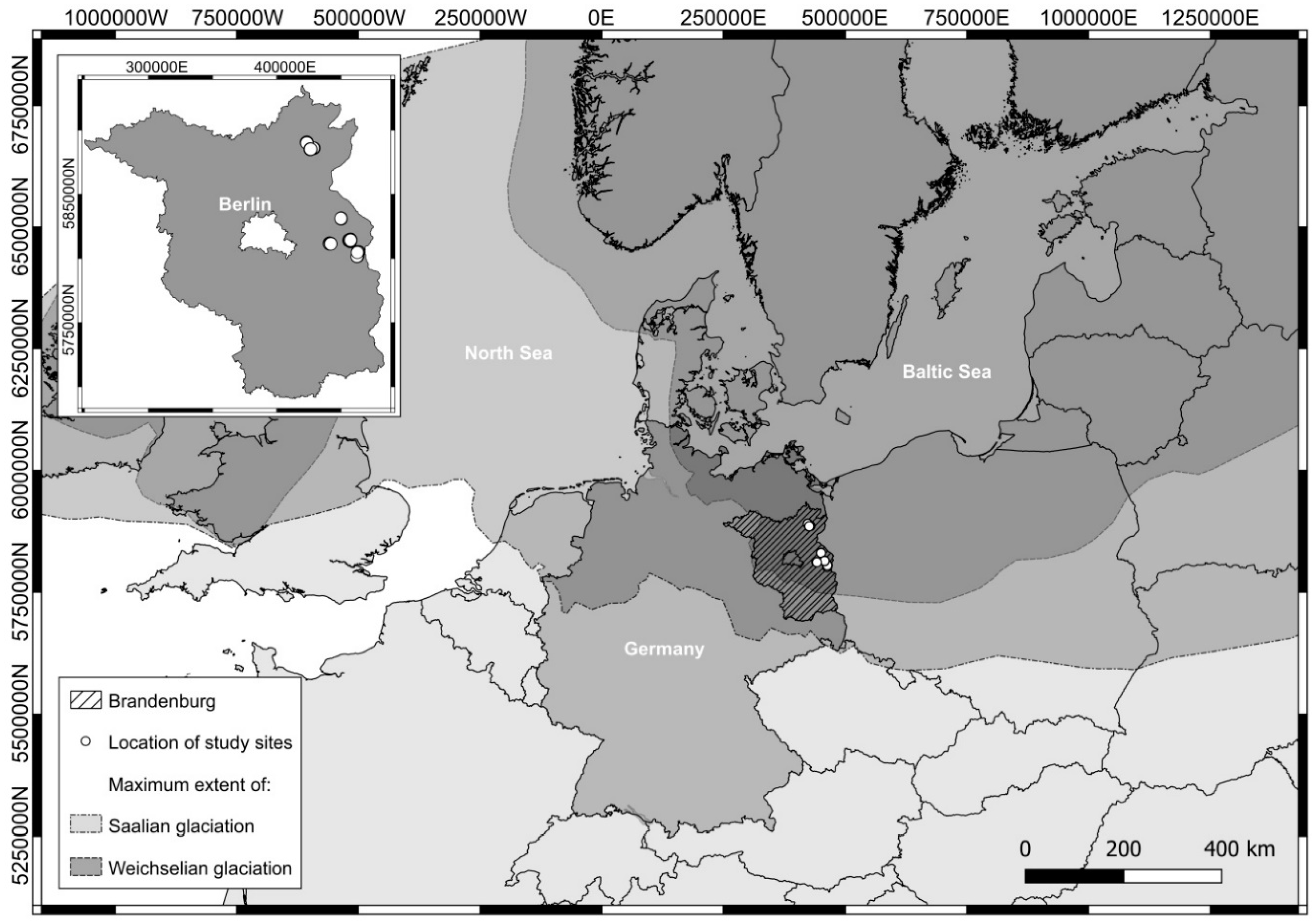
2.1. Site Description

Agricultural fields were studied in the north-east German Plain, which is part of the broader geomorphological region of the North European Plain (Figure 1). It was largely formed by the Pleistocene glaciations of the terrestrial Scandinavian ice sheets as well as by periglacial geomorphic processes. In the study area, the present-day landforms were particularly shaped by the advances of the Weichselian (115–12 ka) and the preceding Saalian glacial belt (150–130 ka; [32]). Climatically, it is situated in a transitional zone between the oceanic climate of Western Europe and the continental climate of Eastern Europe. Due to a relatively low altitudinal range of the land surface of ~0–200 m a.s.l., orography does not introduce relevant climatic differences. Thus, following the Koeppen–Geiger climate classification system, the climate of the study area can be classified as temperate oceanic with an increasing influence of continental circulations. The mean annual air temperature is around 9 °C. The coldest and warmest months are January and July with mean temperatures of −1 and 18 °C, respectively. With a mean annual total precipitation of less than 550 mm, it is one of the driest regions in Germany.

In the present study, eleven fields of three farms were analyzed (Figure 1). They are situated in the east and in the north of the federal state of Brandenburg, which is located in the Pleistocene young morainic landscape of the Weichselian glaciation as well as in the Holocene river valley of the Oderbruch. The fields studied well represent the agricultural land in Brandenburg that is characterized by a high in-field soil variability. Furthermore, they can exhibit both too low (acidic) as well as too high (alkaline) pH values.

2.2. Standard Laboratory Analyses of Studied Soils

To determine the LR according to the standard VDLUFA guidelines and to characterize the studied soils regarding their acidity-affecting soil properties, the following laboratory analyses were carried out on oven-dried (75 °C) and sieved (<2 mm) soil samples:

• The soil pH value was measured in 10 g of soil and 25 mL of 0.01 M CaCl₂ solution following DIN ISO 10390. The pH was measured with a glass electrode after a reaction time of 60 min;
• The particle distribution of the fraction <2 mm was determined according to the German standard in soil science (DIN ISO 11277) by wet sieving and sedimentation after removal of the organic matter with hydrogen peroxide (H₂O₂) and dispersal with 0.2 N sodium pyrophosphate (Na₄P₂O₇);
• Soil organic carbon (SOC) was analyzed by elementary analysis using the dry combustion method (DIN ISO 10694) after removing inorganic carbon with hydrochloric acid. Finally, the amount of SOM was calculated following Equation (1) [36]:

$$SOM[\%]=SOC[\%]·1.72$$

(1)

2.3. LR Based on Base Neutralizing Capacity (LR_BNC)

A total of 420 soil samples were analyzed for the base neutralizing capacity (BNC). The BNC is defined as the amount of soil acidity that is neutralized by a base in a given time interval to a certain pH value [11]. To directly determine the LR of the studied soils, based on their base neutralizing capacity (LC_BNC), we followed the protocol of Meiwes et al. [11] (see also [37]). The method essentially consists of the addition of varying concentrations of a base to aliquots of the soil sample. The resulting pH changes are recorded along with the base concentration added. With these data points, a continuous titration curve can be fitted which is used to determine the amount of base required to raise the pH value of that soil to a certain level.

In detail, the protocol included the following steps: the soil samples were air-dried, and where necessary, the soil aggregates were manually crushed before passing them through a 2 mm screen. Then, 150 g sample was divided into six subsamples of 25 g. One of these subsamples served as a control and was mixed with 50 mL deionized water, while the other subsamples were mixed with 25 mL 2 N CaCl₂ and 25 mL 8 N NaOH solutions of five concentrations. This yielded six concentration levels of Ca(OH)₂ added to the soil: 0, 0.25, 0.5, 1.25, 2.5 and 5 mmol_c (25 g soil)⁻¹. By adding Ca²⁺ and Na⁺ ions to the soil solution, H⁺ and Al³⁺ ions are desorbed from the surface of soil colloids and neutralized by OH^- ions. After 18 h of mechanical shaking the pH values were measured with a glass electrode (WTW SenTix^® 81, Xylem Analytics, Weilheim, Germany) in the supernatant solution. For the quantification of the buffering, the pH values and their corresponding concentrations of Ca(OH)₂ added were displayed in a scatterplot and a titration curve was fitted to the six points. Based on the model, the amount of Ca(OH)₂ in mmol_c (25 g soil)⁻¹ to achieve a target pH of 6.5 was derived and converted to kg CaCO₃ (ha*dm)⁻¹ by multiplying by 2000 [11,38]. Because fertilization guidelines for the UK [38] and most other countries advice to maintain a soil pH of 6.5 for cropped land [6], this was chosen as the target pH value. Of course, this does not reflect the fact that arable crops differ in their sensitivity to soil acidity.

2.4. LR Based on VDLUFA Guidelines (LR_VDLUFA)

The best management practice of liming in Germany is given by the Association of German Agricultural Investigation and Research Institutions (VDLUFA) [25]. The procedure is based on 30 years of fertilization trials studying the relationship between soil pH and yield [26,27,28,29]. The LR_VDLUFA indirectly estimates the LR of a soil based on its current pH value, soil texture and SOM content as they are related to soil–buffer capacity. Whereas the pH value is lab-analyzed, in practice, the soil texture and SOM are mostly estimated. A categorical classification scheme in terms of a look-up table is used to define a target pH range of the management unit from the classes of soil texture and SOM content, and determines the LR from the current pH value. Within the classes formed by texture and SOM, it is assumed that the pH changes linearly with the addition of pure lime:

$$LR \left[\frac{dt CaO}{ha}\right]=a+b\ast pH$$

(2)

where the regression coefficients a and b depend on the texture of the soil. For characterizing the pH conditions qualitatively, five pH classes are distinguished regarding LR and particular soil conditions, such as, nutrient availability and pollutant mobility, as well as soil structure and soil fertility (

Table 1. Soil pH and the lime requirement classes from the Association of German Agricultural Investigation and Research Institutions (VDLUFA) guidelines valid for Germany [25].

pH Class	Lime Supply	Lime Requirement
A	Very low	Recovery liming
B	Low	Buildup liming
C	Optimal	Maintenance liming
D	High	No liming
E	Very high	No liming and no use of fertilizers that react physiologically or chemically alkaline

).

It is important to note that the VDLUFA recommendation algorithm accounts formaintenance or conservation liming. This is a basic lime rate which should be applied even in cases when the pH value is in its optimal range (see Table 1 pH class C). The maintenance rate should secure that the pH value stays in an optimum range until the next lime application at the beginning of the next crop rotation in three to six years.

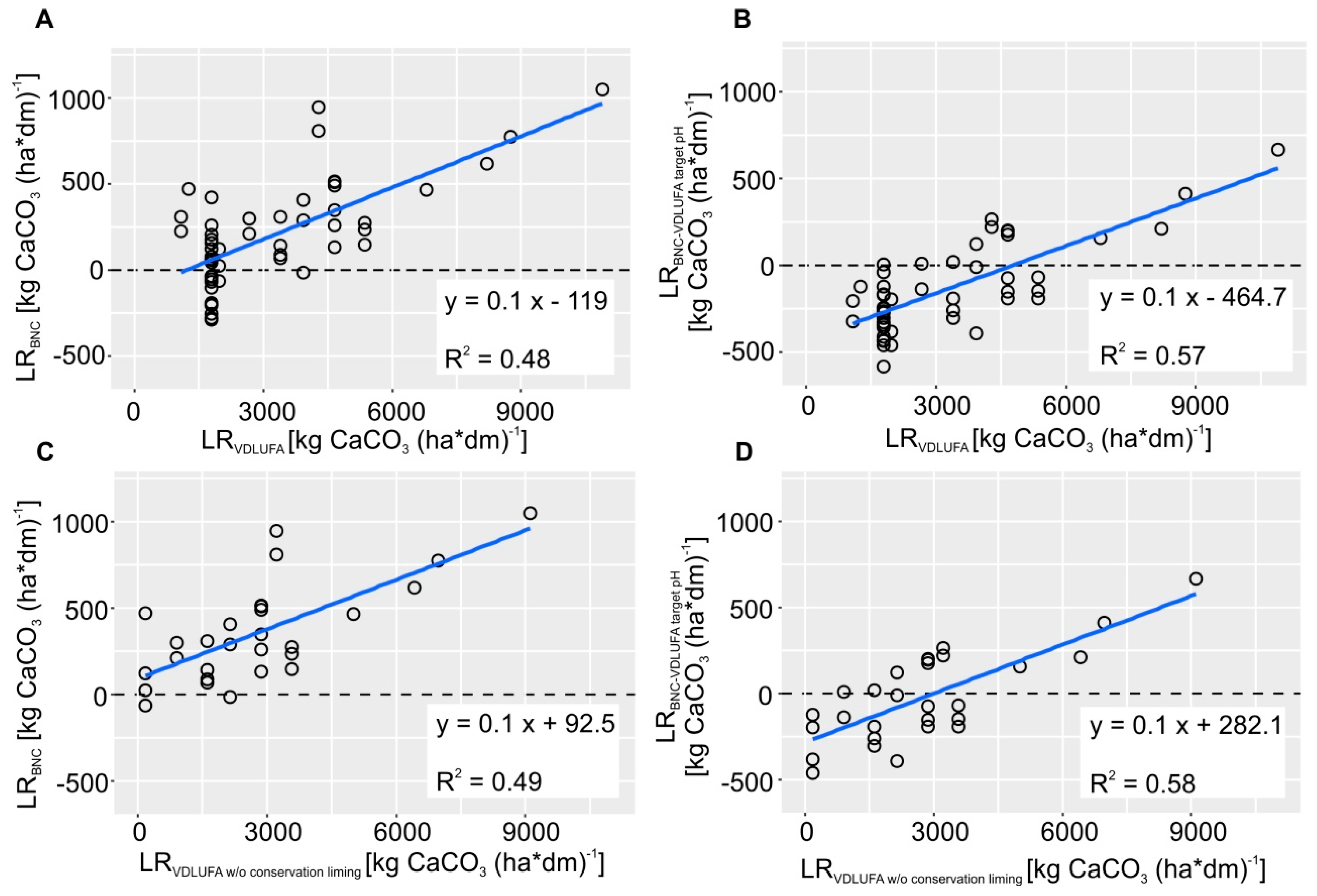
2.5. Comparison between LR_BNC and LR_VDLUFA

In a subsequent step, the lime recommendations based on the base neutralizing capacity (LR_BNC) are to be compared with the VDLUFA standard procedure for lime fertilization in Brandenburg (LR_VDLUFA). As the VDLUFA method quantifies LR in kg CaO ha⁻¹, it was converted to kg CaCO₃ ha⁻¹ using a conversion factor of 1.786. Furthermore, the two methods assume different bulk densities of the soil (VDLUFA: 1.2–1.5 g cm⁻³; BNC: 1.0 g cm⁻³). Hence, the LR_BNC was corrected by a factor of 1.35. Moreover, one major difference between the two methods must be accounted for: as mentioned above, the BNC method identifies one freely selectable target pH value whereas the VDLUFA method recommends an optimum pH range that is a function of texture and SOM content of the respective soil sample. To overcome this disparity, we also calculated the LR_BNC for the target pH values that were identified by the VDLUFA method using the arithmetic mean of the minimum and maximum values of the optimum pH range (LR_{BNC(VDLUFA target pH)}).

2.6. Titration Curve Fitting and Statistical Analysis

All the data were processed with the free software environment for statistical computing and graphics R (version 3.6.1) [39]. To fit a BNC curve to the six titration points, non-linear regression modeling was conducted using the nls function. To analyze the correlations between the BNC parameters and the soil properties that are well known to affect soil acidity and LR, univariate (ULR) and multi-variate linear regression (MLR) analyses were conducted. In the case of non-linear relationships between two variables, we transformed one variable in order to linearize the relation. For the SOM content, we applied a log transformation. As the three particle size fractions clay, silt, and sand are compositional data that sum up to 100%, a log-ratio transformation was conducted [40,41]. In order to quantify the degree of association between two variables while removing the controlling effect of others, we computed the partial correlation using Spearman’s rank correlation coefficient (Spearman’s Rho). In the MLR analysis, the importance (sensitivity) of the predictor variables was evaluated by computing standardized regression coefficients (SRCs). For this, the input data were standardized before conducting the MLR analysis by subtracting the sample mean from the original values and dividing by the sample’s standard deviation. This removes the influence of the different scales of the covariates on the estimation of the regression coefficients. The magnitudes of the SRCs are direct measures of sensitivity, i.e., the influence of an independent variable on the model as a whole [42]. The performance of the regression models was quantified using the coefficient of determination (R²).

3. Results and Discussion

The descriptive statistics of the laboratory results of soil reference samples as well as the results of the base neutralizing capacity (BNC) analysis are shown in

Table 2. Descriptive statistics of the laboratory results of reference soil samples as well as of the base neutralizing capacity (BNC) data.

		n	Minimum	Mean	Median	Maximum	Standard Deviation
Standard soil data	pH	360	3.9	6.1	6.2	7.4	0.7
	SOM * (%)	100	0.8	1.6	1.4	5.6	0.8
	Clay (%)	190	1.0	12.2	9.5	46.0	8.9
	Silt (%)	190	2.0	22.3	23.8	37.9	8.3
	Sand (%)	190	30.0	65.5	65.6	97.0	13.5
BNC data **	pH0	420	4.5	6.7	6.7	8.0	0.6
	pH0.25	420	5.6	7.5	7.4	9.7	0.6
	pH0.5	420	6.1	8.2	8.1	10.3	0.7
	pH1.25	420	7.0	9.8	9.8	11.6	0.7
	pH2.5	420	8.2	11.2	11.3	12.0	0.5
	pH5	420	9.1	12.1	12.1	12.4	0.3
	δpHtotal	420	2.5	5.4	5.4	7.6	0.7
	α	420	11.1	12.5	12.4	13.8	0.3
	β	420	4.1	5.8	5.8	8.5	0.8
	γ	420	0.1	0.5	0.5	0.9	0.1

* SOM: soil organic matter; ** pH₀: initial pH value measured in deionized water; pH_0.25, pH_0.5, pH_1.25, pH_2.5 and pH₅: pH values after the addition of respective amounts of Ca(OH)₂ (mmol_c (25 g soil)⁻¹); δpH_total: total pH increase over all the base additions; α, β, γ: parameters of the exponential regression model.

. The pH of the soils ranged between 3.8 (extremely acidic) and 7.4 (slightly alkaline) with median values of 6.2 (slightly acidic). The content of SOM was rather low throughout the study region, having minima of 0.8%, maxima of 5.6% and median values of 1.4%. The dominating soil texture classes (following the German Soil Texture Classification System KA5; [43]) of the soils studied are: loamy sand (56%) and silty sand (17%) whereas clayey loam (9%), clayey sand (7%), sandy loam (7%), pure sand (4%) and loamy clay (0.5%) are of rather sporadic occurrence.

The BNC data show that the initial pH value, which is measured in deionized water (pH₀), ranges between 4.5 and 8.0 with a median of 6.7. The addition of up to 5 mmol_c (25 g soil)⁻¹ Ca(OH)₂ increased the pH successively to 12.1 on average. The difference between the pH0 and pH5 (δpH_total) was 5.4 units on average. The pH increase per mmol_c base added was stronger at lower concentrations and considerably lower at higher concentrations.

The pH reacts non-linearly to the application of increasing quantities of Ca(OH)₂ (Figure 2). This can be described by an exponential model:

$$pH=\alpha -\beta ·{\gamma }^{\mathrm{Ca}{\left(\mathrm{OH}\right)}_2}$$

(3)

where α, β and γ are the regression coefficients of the exponential function. The exponential model is commonly used in soil science in the description of the kinetics of chemical reactions including titration and buffer curves [44,45]. In the range of Ca(OH)₂ applied, the pH response did indicate the presence of not more than one buffering system which could have necessitated the fitting of a more complex model (for titration curves which show the buffering of exchangeable H⁺ and Al₃⁺ the reader is referred to Sparks [44]). Depending on the differences in the soil acidity and the pH buffer capacity (pHBC), the titration curves of our samples varied as illustrated in Figure 2A. The coefficients of the model can be understood as follows: whereas α represents the threshold value to which the pH can maximally increase Figure 2B), the term α − β is the starting point of the graph at the axis of ordinates. β, on the other hand, is described by the difference from the starting point to the end point of the titration curve. Finally, γ represents the sensitivity of the buffer system. When γ is close to 0, the curve exhibits a strong concavity with a steep ascent (Figure 2A, curve a). When γ is close to 1, the ascent is gentle and the curve is almost linear (Figure 2A, curve c; Figure 2B). The parameter γ particularly characterizes the pHBC of the soils. This can be seen in Table 2, where the standard deviation of the pH response increases from pH₀ to pH_1.25. Correspondingly, in Figure 2 one can observe the differences in the concavity and the exponential part of the curves characterizing the strongest pH increase in the course of the curve due to the different pHBCs of the investigated soils. In the subsequent saturation phase of the curve (pH_2.5 and pH₅), when the pH change decreases, the standard deviation decreases (Table 2). Summery statistics of the BNC model parameters α, β and γ can be found in. Furthermore, it is of interest whether the parameters vary independently from each other or whether they contain redundant information about the pH buffering. In

Table 3. Correlation matrix of the regression coefficients of the exponential function using Spearman’s Rho.

	α	β	γ
α		0.85	0.57
β	0.85		0.44
γ	0.57	0.44

Spearman’s Rho is shown as an indicator of the correlations between the model parameters. Correlations between α and γ as well as β and γ are weak, indicating that these parameters are largely independent. The correlation of parameters α and β is much stronger. This can be explained by the fact that α and β form an interaction term in the model (Equation (3)). Visually, one can observe this interaction in Figure 2B, which shows that both parameters affect the starting point of the curve at the y axis and thus, they cannot be completely independent from each other.

The exponential shape of the measured titration curves are not in line with earlier studies, which reported an approximately linear relationship between lime application and pH response for the pH range from 4.5 to 6.5 [14,46,47,48]. However, for wider pH ranges near and above pH 6.5, other authors like Sparks [44] or Sposito [45] described a non-linear pH response. Furthermore, Liu et al. [14] found that for 60% of their titrations performed in deionized water, the initial pH before adding Ca(OH)₂ was lower than the intercept of the linear regression model. This, as well as the course of titration points illustrated in Liu et al. [14] suggests that a better fit could be obtained by an exponential rather than a linear model. However, this only becomes obvious when a wider range of pH responses is induced as it was done in the present study. Süsser and Schwertmann [49], Sparks [44], Sposito, and others stated that the individual shape of the titration curve depends on the characteristics and concentrations of proton-buffering substances in the soil. A list of buffering substances, buffer reactions and main pH ranges of buffering can be found in Schwertmann et al. [50]. According to Süsser and Schwertmann [49], soils rich in SOM show a rather linear graph, i.e., the BNC increase is nearly constant over a wider pH range from 2.5 to 7. This is because the acid strength of functional groups of humic substances is evenly distributed over this pH range. On the contrary, soils poor in SOM show non-linear titration curves. The latter applies to our studied soils, showing low amounts of SOM of median values of 1.4%.

Hue and Ikawa [51] also found exponential lime requirement curves in a study of acid soils from Hawaii. Nelson and Su [52] studied pHBC in acidic tropical soils and found non-linear titration curves with an exponential shape for pH values above 4–5. However, at a pH value below 4–5, they observed a dramatic increase in the pHBC resulting in an actually sigmoidal graph. Magdoff and Bartlett [53] also discovered sigmoidal titration curves for soils of Vermont (USA) with high pHBCs below pH 4 and above pH 7. This pHBC increase at low pH values was not observed in the present study due to a lack of strongly acidic soils.

The pHBC of a soil quantifies its ability to resist pH changes upon the addition of H⁺ or OH⁻ ions through neutralization reactions with a buffer substance. The change in pH depends on both the initial pH value as well as the capacity of the buffer substance. As long as the buffer substance is not completely depleted, the pH will not change considerably [4]. The pHBC is expressed in moles of acid/base needed to change the pH by one unit (mmol_c kg⁻¹ pH⁻¹). Consequently, it can be directly deduced from the titration curve. As the BNC titration curve has a non-linear form, the pHBC is not constant over the entire pH range as it would be for a linear model (see [54]). Thus, it is expressed as follows:

$$pHBC \left[mmo{l}_c k{g}^{-1} p{H}^{-1}\right]=\left(\frac{\log \left(\frac{\alpha -p{H}_2}{\beta }\right)}{\log \left(\gamma \right)}\right)-\left(\frac{\log \left(\frac{\alpha -p{H}_1}{\beta }\right)}{\log \left(\gamma \right)}\right); for p{H}_b-p{H}_a=1$$

(4)

where α, β and γ are the regression coefficients and pH_a and pH_b are the lower and the upper boundary of the pH increase of interest, whereas pH_b − pH_a = 1. This implies that the pH change through liming is strongest at low soil pH values and pHBCs, and exponentially decreases towards a threshold value at higher pH values and pHBCs. It has to be emphasized that the agronomically relevant section of the titration curves up to pH 7 are well below that region of saturation where LR increases significantly (see Figure 2). However, for all 420 soil samples analyzed, the median LR increases from 394 to 449 and from 449 to 524 kg CaCO₃ ha⁻¹ to achieve a pH increase from pH 4 to 5, 5 to 6, and 6 to 7, respectively.

As the difference of the regression coefficients, α − β, describes the starting point of the graph, it is a function of the initial pH measured in deionized water (pH₀; Figure 3A). β, on the other hand, Figure 3B). Furthermore, the lower the pH_0, or α − β, respectively, the higher the total pH increase over all five base additions (Figure 3B).The δpH_total is affected by the soil’s pHBC showing higher values at lower pHBCs and vice versa.

In a subsequent step, the BNC parameters were correlated with soil properties that are known to affect soil acidity and pHBC, i.e., pH, SOM and soil texture [54]. This is done by means of bivariate partial correlation (

Table 4. Spearman’s rank correlation coefficient of the partial correlation between the BNC parameters and the soil acidity and pH buffer capacity affecting soil properties (pH, SOM, Clay and sand).

	pH	SOM *	Clay **	Sand **
δpHtotal °	−0.91	−0.31	−0.22	−0.14
α	−0.84	0.18	−0.02	0.09
β	−0.92	0.27	−0.25	0.01
γ	−0.77	0.63	0.22	−0.24
LRBNC °°	−0.89	0.11	−0.35	−0.01

* log-transformed; ** log-ratio-transformed; ° δpH_total: the total pH increase over all five base additions; °° LR_BNC: BNC-based lime requirement.

) as well as standardized regression coefficients (SRC) from MLR models (

Table 5. Standardized regression coefficients (SRC) BNC parameters and the soil acidity and pH buffer capacity affecting soil properties pH, SOM, Clay and sand. Numbers in brackets indicate the sensitivity ranking.

	pH	SOM *	Clay **	Sand **
δpHtotal	−0.70	−0.18	−0.07	−0.05
α	−0.60	0.06	0.02	0.07
β	−0.82	0.07	−0.10	−0.01
γ	−0.60	0.50	0.10	−0.17
LRBNC	−0.77	0.00	−0.19	0.02

* log-transformed; ** log-ratio-transformed.

). Both results clearly show that for all BNC parameters, high correlations as well as sensitivities exist for the soil pH, whereas the association with SOM and soil texture are rather negligible. Consequently, the pH value is by far the most important soil parameter to characterize the pHBC and lime requirement of the investigated soils. This confirms the importance of regular soil pH measurements. A certain exception is the association with γ where SOM received a comparatively high Spearman’s Rho and SRC value, respectively. This indicates that the concavity of the titration curve, respectively the soil’s pHBC, is equally controlled by pH and SOM: the lower the pH and the higher the SOM content, the larger is γ. This confirms the statement by Süsser and Schwertmann [49] that soils rich in SOM show a rather linear titration curve with γ close to 1.

The higher sensitivity of SOM compared to the soil texture is, at first sight, surprising, since the amounts of SOM are rather low throughout the study region. However, as explained by Stevensen [55] and Bloom [54], pH-dependent protonation and deprotonation is governed by carboxylic groups in humic acids. Accordingly, Magdoff and Bartlett [53], Mikkelsen [56] (2005) and Nelson and Su [52] observed pronounced correlations between the pHBC and SOM.

The MLR models with the explanatory variables pH, SOM, clay, and sand were used for the sensitivity determination. However, the best performance in the prediction of BNC parameters was often achieved by the MLR models with a lower number of predictors (Figure 4). The prediction performance was reasonable for γ (R² = 0.62) and good for β (R² = 0.82), LR_BNC (R² = 0.82) and δpH_total (R² = 0.85). The prediction model for α yielded a lower R² of 0.49. This was caused by the leverage of some very low and very high α values which cannot be explained well by the predictors in consideration. Furthermore, all the prediction models have in common that they slightly underestimate high and overestimate low values.

Finally, the LR was determined based on the VDLUFA standard procedure for lime fertilization in Brandenburg (LR_VDLUFA) to be compared with LR_BNC. There are two major differences between the two LR methods. Firstly, LR_BNC can be determined for a freely selectable target pH allowing for an adaptation of liming to specific crop demands, whereas LR_VDLUFA is calculated for a pH optimum that depends on the texture and SOM content designated as a discrete classification system. Secondly, LR_BNC also defines negative LR values providing useful information on the magnitude of soil acidification necessary when a soil has a too high pH value. On that basis, the farmer is able to evaluate if these sections of the field are simply left out of lime treatment or if it is needed to actively acidify the soil to increase soil productivity, e.g., by applying fertilizers that react physiologically or chemically acidic. With respect to economics, it should be considered that LR_BNC does not require the expensive analysis of soil texture and SOM as this is the case with the VDLUFA algorithm. On the other hand, however, if data on texture and SOM are available, only measuring the pH is all that the VDLUFA algorithm needs for calculating the LR while the BNC determination is more laborious and time consuming. Maybe new developments in proximal soil sensing can overcome these shortcomings [57].

As Figure 5A and B illustrate, the LR_VDLUFA correlates well with the LR_BNC and LR_{BNC(VDLUFA target pH)}, respectively. As the latter takes into account the VDLUFA target pH values, it received a higher R² of 0.57 compared to 0.48 when considering a fixed target pH of 6.5. It is noticeable from the scatterplots that the VDLUFA applies a categorical classification scheme in order to determine the LR whereas LR_BNC is continuous. Consequently, from Figure 5A, it can be seen that a LR_BNC range from −289 to 420 kg CaCO₃ ha⁻¹ is associated with a single LR_VDLUFA value of 1786 kg CaCO₃ ha⁻¹. Furthermore, due to that categorical classification, the VDLUFA scheme sometimes produces rather erratic changes in LR at class boundaries of soil texture and SOM, which are technically and scientifically not justified. The development of a continuous and stepless VDLUFA algorithm for LR calculation could overcome this situation.

From the equations of the two regression models of Figure 5A,B, the difference between the LR_BNC and LR_VDLUFA can be quantified. As the slope of the regression line has a value of 0.1, LR_VDLUFA is approximately one order of magnitude higher than the LR_BNC. Furthermore, from the intercept it can be stated that a constant surcharge of 119 and 465 kg CaCO₃ ha⁻¹ needs to be added to the LR_BNC and LR_{BNC(VDLUFA target pH)}, respectively, to obtain the same rates as the LR_VDLUFA. Three main reasons can explain the higher LR_VDLUFA values. First, the VDLUFA adopts a concept of maintenance or conservation liming, which recommends applying lime even when the pH value is already in its optimal range. The intention of this approach is to sustain the optimum pH until the next lime application is due, during the next rotation in three to six years. The rates for conservation liming range between 536 and 3572 kg CaCO₃ ha⁻¹ with lower values for sandy soils rich in SOM and higher values for clayey soils poor in SOM [25]. The BNC method, on the other hand, only determines the LR necessary to reach the target pH value but not to preserve it over a longer period of time.

Conservation liming aims at compensating calcium losses due to soil acidifying processes such as leaching and the removal of nutrients, as well as the input or formation of acids. These Ca losses range between 180 and 1250 kg CaCO₃ ha⁻¹, depending on the crop type (farmland, grassland), soil texture and annual precipitation (

Table 6. Calcium losses due to neutralization and leaching in kg CaCO₃ ha⁻¹ (after [58]; modified).

		Annual Precipitation
Soil Texture	Crop Type	Low (<600 mm)	Medium (600–750 mm)	High (>750 mm)
Sandy soils	Farmland	540	710	890
	Grassland	270	450	630
Loamy soils	Farmland	710	890	1070
	Grassland	360	540	710
Clayey soils	Farmland	890	1070	1250
	Grassland	450	630	800

). When a liming cycle of three years is considered, these values correspond well with the range of conservation liming rates suggested by the VDLUFA protocol. Subtracting the respective amount of conservation liming from LR_VDLUFA reduces the differences of LR_BNC and LR_{BNC(VDLUFA target pH)} to −92 and 282 kg CaCO₃ ha⁻¹, respectively. Furthermore, it very slightly increases the R² of the respective regression models to 0.49 and 0.58 (Figure 5 C,D).

A second reason for higher LR_VDLUFA values results from the development of the VDLUFA method on the bases of field trials. Hence, the estimation of the pH-buffering effect of the soil as well as the liming effect on soil acidity and yield development were investigated in an open system, i.e., natural soil acidifying processes taking place in the soil during the experiment that have an influence on the reaction of lime and the development of soil acidity are included. Consequently, the pH effect of liming is expected to be depressed by these factors resulting in higher lime recommendations. On the contrary, the BNC method was solely developed on the basis of laboratory analyses. Here, the LR estimation is carried out in a closed system, i.e., processes like the leaching of bases, acid rain or nutrient uptake by plant roots are excluded.

The third reason can be found in the preparation of the soil samples. For BNC, the soil samples are standardized by drying and sieving and are exposed to the basic solution for the entire trial period. Thus, in the laboratory experiments, the chemical reactions triggered by the addition of bases can run more effectively and completely. These results in an underestimation of the LR following the BNC method compared to the VDLUFA method. Using the regression models shown in Figure 5, LR_BNC can be converted into LR_VDLUFA. However, additional research should be done in order to develop a sound scientific model that adjusts LR_BNC by realistic values of annual Ca²⁺ removal and acidification by natural processes and N fertilization. Furthermore, further BNC studies should be carried out in different soilscapes.

4. Conclusions

In the present paper, the base neutralizing capacity (BNC) of 420 samples from a quaternary landscape in Central Europe (north-east Germany) were analyzed in order to characterize the soils regarding their pH buffer capacity and determine their lime requirement (LR). Since pH and pH buffering are key factors for many soil processes, it is important to regard them in research as well as in practical decision making. The detailed, otherwise hard-to-get information about the pH buffer capacity of soils in this region, might aid scientists and advisors in their work. An important application of data on pH buffering is the determination of lime requirements. Thus, the BNC data were correlated with soil properties that are well known to affect soil acidity, i.e., pH, soil texture and SOM. It could be shown that the current pH value has the highest impact on the BNC-based determination of lime requirement. Thus, it is of uttermost importance to regularly measure soil pH. From the soil acidity perspective, it is also of great importance to manage SOM in these poor soils, since SOM contributes much more to the buffering than soil texture. The BNC-based lime requirement (LR_BNC) was compared with the LR following the VDLUFA standard procedure for lime fertilization in Germany (LR_VDLUFA). One big difference is that the LR_BNC also gives information on the amount of soil acidification needed when the soil pH is too high. This is important because soils developed on glacial till often contain natural lime. In this regard, practitioners should know that the LR_VDLUFA is generally higher than LR_BNC, which is partly the result of a maintenance or conservation liming that is included in the LR_VDLUFA approach to keep an optimum pH in a longer term. This concept is reasonable for managing acidic soils but not for calcareous soils. It would be favorable to combine conservation liming for soils with a positive LR_BNC. Furthermore, to better value the VDLUFA approach, one should bear in mind that the algorithm was primarily derived from field experiments where natural soil acidifying and management practices reduced the effect of lime treatment. We conclude that the evaluation of the BNC could be a suitable method (or addition) to determine the LR since it integrates more comprehensive information about the direct response to lime application. Thus, it may allow better adapting pH management to individual soils. Since this study is based on laboratory analyses only, it requires field trials to compare both approaches under practical conditions.

References

1. Robson, A.D. Soil Acidity and Plant Growth; Academic Press: Sydney, NSW, Australia, 1989. [Google Scholar]
2. Mengel, K.; Kirkby, E.A. Principles of Plant Nutrition, 5th ed.; Kluwer Academic Publishers: Dordrecht, The Netherlands, 2001. [Google Scholar]
3. Epstein, E.; Bloom, A.J. Mineral Nutrition of Plants: Principles and Perspectives, 2nd ed.; Sinauer Associates: Sunderland, MA, USA, 2001. [Google Scholar]
4. Blume, H.-P.; Bruemmer, G.W.; Fleige, H.; Horn, R.; Kandeler, E.; Koegel-Knabner, I.; Kretzschmar, R.; Stahr, K.; Wilke, B.-M. Scheffer/Schachtschabel Soil Science; Springer: Heidelberg, Germany, 2016; p. 618. [Google Scholar]
5. Pagani, A.; Sawyer, J.E.; Mallarino, A.P.; Moody, L.; Davis, J.; Phillips, S. Site-Specific Nutrient Management For. Nutrient Management Planning To Improve Crop. Production, Environmental Quality, and Economic Return: Module 8—Soil pH and Lime Management; U.S. Department of Agriculture—Natural Resources Conservation Service (USDA-NRCS): Washington, DC, USA, 2017. Available online: http://www.nutrientstewardship.com/training/ (accessed on 6 January 2020).
6. Goulding, K.W. Soil acidification and the importance of liming agricultural soils with particular reference to the United Kingdom. Soil Use Manag. 2016, 32, 390–399. [Google Scholar] [CrossRef] [PubMed]
7. Holland, J.; Bennett, A.; Newton, A.; White, P.; McKenzie, B.; George, T. Liming impacts on soils, crops and biodiversity in the UK: A review. Sci. Total Environ. 2018, 610, 316–332. [Google Scholar] [CrossRef] [PubMed]
8. Mengel, K.; Kirkby, E.A. Principles of Plant Nutrition; Kluwer Academic Publishers: Dordrecht, The Netherlands, 2001; p. 849. [Google Scholar]
9. Sims, J.T. Lime Requirement. In Methods of Soil Analysis—Part 3: Chemical Methods; Bigham, J.M., Bartels, J.M., Eds.; Soil Science Society of America Book Series; John Wiley & Sons, Inc.: New York, NY, USA, 1996; Volume 5, p. 670. [Google Scholar]
10. Dunn, L.E. Lime-requirement of soils by means of titration curves. Soil Sci. 1943, 56, 341–352. [Google Scholar] [CrossRef]
11. Meiwes, K.J.; Koenig, N.; Khana, P.K.; Prenzel, J.; Ulrich, B. Chemical test methods for mineral soils, litter layers and roots to characterize and evaluate acidification in forest soils (In German: Chemische Untersuchungsverfahren für Mineralboden, Auflagehumus und Wurzeln zur Charakterisierung und Bewertung der Versauerung in Waldböden). In Die Erfassung des Stoffkreislaufs in Waldökosystemen—Konzeption und Methodik, Berichte des Forschungszentrums Waldökosysteme/Waldsterben, Bd. 7; Meiwes, K.-J., Hauhs, M., Gerke, H., Asche, N., Matzner, E., Lammersdorf, N., Eds.; Institut für Bodenkunde und Waldernährung der Universität Göttingen: Göttingen, Germany, 1984. [Google Scholar]
12. Alley, M.; Zelazny, L. Soil Acidity: Soil pH and Lime Needs. In Soil Testing: Sampling, Correlation, Calibration, and Interpretation, Proceedings of the Annual Meeting of the American Society of Agronomy and Soil Science Society of America, Chicogo, IL, USA, 1–5 December 1985; Brown, J.R., Ed.; Soil Science Society of America, Inc.: Madison, WI, USA, 1987; pp. 65–72. [Google Scholar]
13. McLean, E. Principles underlying the practice of determining lime requirements of acid soils by use of buffer methods. Comm. Soil Sci. Plant. Anal. 1978, 9, 699–715. [Google Scholar] [CrossRef]
14. Liu, M.; Kissel, D.E.; Cabrera, M.L.; Vendrell, P.F. Soil Lime Requirement by Direct Titration with a Single Addition of Calcium Hyroxide. Soil Sci. Soc. Am. J. 2005, 69, 522–530. [Google Scholar] [CrossRef]
15. Kissel, D.E.; Isaac, R.A.; Hitchcock, R.; Sonon, L.S.; Vendrell, P.F. Implementation of soil lime requirement by a single-addition titration method. Commun. Soil Sci. Plant. Anal. 2007, 38, 1341–1352. [Google Scholar] [CrossRef]
16. Thompson, J.S.; Kissel, D.E.; Cabrera, M.L.; Sonon, L.S. Equilibration reaction from single addition of base to determine soil lime requirement. Soil Sci. Soc. Am. Proc. 2010, 74, 663–669. [Google Scholar] [CrossRef]
17. Alabi, K.E.; Sorensen, R.C.; Knudsen, D.; Rehm, G.W. Comparison of several lime requirement methods on course textured soils of Northeastern Nebraska. Soil Sci. Soc. Am. J. 1986, 50, 937–941. [Google Scholar] [CrossRef]
18. Owusu-Bennoah, E.; Acquaye, D.K.; Mahamah, T. Comparative study of selected lime requirement methods for some acid Ghanaian soils. Commun. Soil Sci. Plant. Anal. 1995, 26, 937–950. [Google Scholar] [CrossRef]
19. Shoemaker, H.E.; Mclean, E.O.; Pratt, P.F. Buffer methods for determining lime requirement of soils with appreciable amounts of extractable aluminum. Soil Sci. Soc. Am. Proc. 1961, 25, 274–277. [Google Scholar] [CrossRef]
20. Adams, F.; Evans, C.E. A rapid method for measuring lime requirement of red-yellow podzolic soils. Soil Sci. Soc. Am. Proc. 1962, 26, 355–357. [Google Scholar] [CrossRef]
21. Mehlich, A. New buffer pH method for rapid estimation of exchangeable acidity and lime requirement of soils. Commun. Soil Sci. Plant. Anal. 1976, 7, 637–652. [Google Scholar] [CrossRef]
22. Viscarra Rossel, R.A.; McBratney, A.B. A response surface calibration model for rapid and versatile site-specific lime requirement predictions in southeastern Australia. Aust. J. Soil Res. 2001, 39, 185–201. [Google Scholar] [CrossRef]
23. Pagani, A.; Mallarino, A.P. Comparison of Methods to Determine Crop Lime Requirement Under Field Conditions. Soil Sci. Soc. Am. J. 2011, 76, 1855–1866. [Google Scholar] [CrossRef]
24. Vossen, P. Changing pH in Soil; University of California Cooperative Extension: Davis, CA, USA, 2002. [Google Scholar]
25. von Wulffen, U.; Roschke, M.; Kape, H.-E. Target Values for Soil Fertility Analysis and Guidance, as well as for the Implementation of the Fertilization Ordinance; (In German: Richtwerte für die Untersuchung und Beratung sowie zur fachlichen Umsetzung der Düngeverordnung (DüV): Gemeinsame Hinweise der Länder Brandenburg, Mecklenburg-Vorpommern und Sachsen-Anhalt); Landesanstalt für Landwirtschaft, Forsten und Gartenbau des Landes Sachsen-Anhalt (LLFG): Bernburg, Germany; Güterfelde, Germany; Rostock, Germany, 2008. [Google Scholar]
26. Kerschberger, M. Ermittlung von Kalkdüngermengen zur Erreichung optimaler pH-Werte des Bodens. Ph.D. Thesis, Institut für Pflanzenernährung Jena der Akademie der Landwirtschaftswissenschaften der DDR, Jena, Germany, 1980; p. 132, Unpublished doctoral dissertation. [Google Scholar]
27. Kerschberger, M. Ermittlung Optimaler Bodenreaktion auf dem Ackerland—Sekundarrohstoffe im Stoffkreislauf der Landwirtschaft und Weitere Beiträge aus den Öffentlichen Sitzungen; VDLUFA-Verlag: Darmstadt, Germany, 1996; Volume 44, pp. 591–594. [Google Scholar]
28. Kerschberger, M.; Deller, B.; Hege, U.; Heyn, J.; Kape, H.; Krause, O. Bestimmung des Kalkbedarfs von Acker-und Grünlandböden; VDLUFA-Verlag: Darmstadt, Germany, 2000. [Google Scholar]
29. Kerschberger, M.; Marks, G. Einstellung und Erhaltung Eines Standorttypischen Optimalen pH-Wertes im Boden—Grundvoraussetzung für Eine Effektive und Umweltverträgliche Pflanzenproduktion; Berichte über Landwirtschaft: Stuttgart, Germany, 2007; Volume 85, pp. 56–77. [Google Scholar]
30. Havlin, J.L.; Tisdale, S.L.; Nelson, W.L.; Beaton, J.D. Soil Fertility and Fertilizers: An Introduction to Nutrient Management; Prentice-Hall, Inc.: Upper Saddle River, NJ, USA, 2005; p. 499. [Google Scholar]
31. Schilling, G. Pflanzenernährung und Düngung; UTB: Stuttgart, Germany, 2000; p. 464. [Google Scholar]
32. Krbetschek, M.R.; Degering, D.; Alexowsky, W. Infrared radiofluorescence ages (IR-RF) of Lower Saalian sediments from Central and Eastern Germany. Zeitschr. Dtsch. Ges. Geowiss. 2008, 133–140. [Google Scholar] [CrossRef]
33. Ehlers, J.; Grube, A.; Stephan, H.J.; Wansa, S. Pleistocene glaciations of North Germany e new results. In Quaternary Glaciations e Extent and Chronology e a Closer Look. Developments in Quaternary Science 15; Ehlers, J., Gibbard, P.L., Hughes, P.D., Eds.; Elsevier: Amsterdam, The Netherlands, 2011; pp. 149–162. [Google Scholar]
34. Winsemann, J.; Brandes, C.; Polom, U.; Weber, C. Depositional architecture and palaeogeographic significance of Middle Pleistocene glaciolacustrine ice marginal deposits in northwestern Germany: A synoptic overview. E G Quat. Sci. J. 2011, 60, 212–235. [Google Scholar] [CrossRef]
35. Moreau, J.; Huuse, M.; Janszen, A.; van der Vegt, P.; Gibbard, P.L.; Moscariello, A. The glaciogenic unconformity of the southern North Sea. In Glaciogenic Reservoirs; Huuse, M., Redfern, J., Le Heron, D.P., Dixon, R.J., Moscariello, A., Craig, J., Eds.; Geological Society of London: London, UK, 2012; pp. 99–110, Special Publication 368. [Google Scholar]
36. Peverill, K.; Sparrow, L.; Reuter, D. Soil Analysis: An Interpretation Manual; CSIRO publishing: Collingwood, VIC, Australia, 1999; p. 369. [Google Scholar]
37. Utermann, J.; Gorny, A.; Hauenstein, M.; Malessa, V.; Müller, U.; Scheffer, B. Geologisches Jahrbuch Reihe G, Band G 8; Schweizerbart´sche Verlagsbuchhandlung: Stuttgart, Germany, 2000. [Google Scholar]
38. Defra. The Fertiliser Manual (RB209); TSO: London, UK, 2010. [Google Scholar]
39. R Core Team. R: A Language and Environment for Statistical Computing; R Foundation for Statistical Computing: Vienna, Austria, 2018; Available online: http://www.R-project.org (accessed on 11 November 2019).
40. Huang, J.; Subasinghe, R.; Triantafilis, J. Mapping particle-size fractions as a composition using additive log-ratio transformation and ancillary data. Soil Sci. Soc. Am. J. 2014, 78, 1967–1976. [Google Scholar] [CrossRef]
41. Muzzamal, M.; Huang, J.; Nielson, R.; Sefton, M.; Triantafilis, J. Mapping soil particle-size fractions using additive log-ratio (ALR) and isometric log-ratio (ILR) transformations and proximally sensed ancillary data. Clays Clay Miner. 2018, 66, 9–27. [Google Scholar] [CrossRef]
42. Saltelli, A.; Ratto, M.; Andres, T.; Campolongo, F.; Cariboni, J.; Gatelli, D.; Saisana, M.; Tarantola, S. Global Sensitivity Analysis: The Primer; John Wiley & Sons: Chichester, UK, 2008. [Google Scholar]
43. Eckelmann, W.; Sponagel, H.; Grottenthaler, W. Bodenkundliche Kartieranleitung KA5, 5th ed.; Bundesanstalt für Geowissenschaften und Rohstoffe in Cooperation with Staatliche Geologische Dienste: Hanover, Germany, 2005. [Google Scholar]
44. Sparks, D. Environmental Soil Chemistry, 2nd ed.; Academic Press, an Imprint of Elsevier: San Diego, CA, USA, 2003. [Google Scholar]
45. Sposito, G. The Chemistry of Soils, 3rd ed.; Oxford University Press: New York, NY, USA, 2016. [Google Scholar]
46. Weaver, A.R.; Kissel, D.E.; Chen, F.; West, L.T.; Adkins, W.; Rickman, D.; Luvall, J.C. Mapping soil pH buffering capacity of selected fields in the coastal plain. Soil Sci. Soc. Am. J. 2004, 68, 662–668. [Google Scholar] [CrossRef]
47. Hoskins, B.R.; Erich, M.S. Modification of the Mehlich lime buff er test. Commun. Soil Sci. Plant. Anal. 2008, 39, 2270–2281. [Google Scholar] [CrossRef]
48. Wolf, A.M.; Beegle, D.B.; Hoskins, B. Comparison of Shoemaker–McLean–Pratt and modified Mehlich buffer tests for lime requirement on Pennsylvania soils. Commun. Soil Sci. Plant. Anal. 2008, 39, 1848–1857. [Google Scholar] [CrossRef]
49. Süsser, P.; Schwertmann, U. Proton buffering in mineral horizons of some acid forest soils. Geoderma 1991, 49, 63–76. [Google Scholar] [CrossRef]
50. Schwertmann, U.; Süsser, P.; Nätscher, L. Proton buffer compounds in soils. J. Plant. Nutr. Soil Sci. 1987, 150, 63–76. [Google Scholar]
51. Hue, N.V.; Ikawa, H. Liming acid soils of Hawaii. University of Hawaii. CTAHR Agron. Soils 1994, 1, 1–2. [Google Scholar]
52. Nelson, P.N.; Su, N. Soil pH buffering capacity: A descriptive function and its application to some acidic tropical soils. Aust. J. Soil Res. 2010, 48, 201–207. [Google Scholar] [CrossRef]
53. Magdoff, F.R.; Bartlett, R.J. Soil pH buffering revisited. Soil Sci. Soc. Am. Proc. 1985, 49, 145–148. [Google Scholar] [CrossRef]
54. Bloom, P.R. Soil pH and pH buffering. In Handbook of Soil Science; Sumner, M.E., Li, Y., Huan, P.M., Eds.; CRC Press: Boca Raton, FL, USA, 2000. [Google Scholar]
55. Stevenson, F.J. Humus Chemistry, 2nd ed.; Wiley: New York, NY, USA, 1994. [Google Scholar]
56. Mikkelsen, R.L. Humic materials for agriculture. Better Crops 2005, 89, 6–10. [Google Scholar]
57. Leenen, M.; Welp, G.; Gebbers, R.; Pätzold, S. Rapid determination of lime requirement by mid-infrared spectroscopy: A promising approach for precision agriculture. J. Plant. Nutr. Soil Sci. 2019, 182, 953–963. [Google Scholar] [CrossRef] [Green Version]
58. BAD. Nährstoffverluste aus landwirtschaftlichen Betrieben mit einer Bewirtschaftung nach guter fachlicher Praxis; Bundesarbeitskreis Düngung: Frankfurt/Main, Germany, 2003. [Google Scholar]
Figure 1. Map of Central Europe with the location of the study sites in the federal state of Brandenburg (Germany) that was largely influenced by the Saalian and Weichselian glaciation at the end of the Pleistocene (Projection: UTM ETRS89 33N) (after [33,34,35]). The inlay map indicates the detailed location of the study sites.
Agronomy 10 00877 g001
Figure 2. Examples of the BNC titration curves: (A) the range of BNC titration curves (a, b, c) from the investigated soils. The solid black line indicates the target pH of 6.5. (B) the influence of the correlation coefficients of the exponential function (α, β, γ) on the shape of the titration curve.
Agronomy 10 00877 g002
Figure 3. Correlations between (A) the BNC regression coefficients α − β and pH0, (B) β and the total pH increase over all five base additions (δpHtotal), and (C) pH0 and δpHtotal.
Agronomy 10 00877 g003
Figure 4. Best-performing multi-variate linear regression (MLR) models in order to predict the BNC parameters (A) δpHtotal, (B) α, (C) β, (D) γ and (E) LRBNC (Claylogratio—log-ratio-transformed clay content, SOMlog—log-transformed SOM content).
Agronomy 10 00877 g004
Figure 5. (A) Comparison between the LRVDLUFA and the LRBNC for a fixed target pH of 6.5, (B) the LRVDLUFA and LRBNC calculated for variable target pH values according to the VDLUFA, (C) the LRVDLUFA without conservation liming and LRBNC for a fixed target pH of 6.5, and (D) the LRVDLUFA without conservation liming and LRBNC calculated for variable target pH values according to the VDLUFA.
Agronomy 10 00877 g005