A Methodological Approach for Irrigation Detection in the Frame of Common Agricultural Policy Checks by Monitoring

Abstract

New needs have arisen from member states and paying agencies (PA) to achieve the compliance assessment from farmers in the frame of the European Common Agricultural Policy (CAP). Traditional field inspection (on-the-spot checks) and computer-aided photointerpretation (CAPI) carried out by each PA over a sample of 5% of the applicants are being replaced by a 100% sample Copernicus satellite-based system (checks by monitoring, CbM). This new approach will be an integral part of the Area Monitoring System that will be part of the Integrated Administrative Control System (IACS) in the post-2020 CAP. Among all the aid schemes having to be analyzed, there are some specific aids in which the detection of irrigation of certain crops can result in a no-compliance resolution. Apart from that, the knowledge of the truly irrigated area in each campaign has always been data of great interest in irrigation planning, crop yield statistics, and water management, and now more than ever. Although several sources of information exist, there is no consensual methodology for estimating the actual irrigated area. The objective of this study is to propose a methodological approach based mainly on Copernicus Sentinel and IACS data not only to detect the surface of herbaceous crops that have been actually irrigated but also to derive a product suitable to be incorporated into the CAP monitoring process system. This methodology is already being used operationally during the ongoing campaign 2020 by Castile and León PA.

1. Introduction

As of 22 May 2018, the European Commission (EC) adopted new rules [1] as a movement to simplify and modernize the EU’s Common Agricultural Policy (CAP) allowing for the first time the usage of a range of modern technologies when carrying out checks for CAP payments. Particularly, these new rules enable data from the EU’s Copernicus Sentinel satellites and other Earth Observation (EO) platforms to be used as evidence when checking farmers’ fulfillment of requirements under the CAP for area-based payments, either direct payments to farmers from European agricultural guarantee fund (first pillar of the CAP) or rural development support payments (second pillar of the CAP). This includes the possibility to completely replace physical checks on farms, the so-called on-the-spot Check (OTSC), with an automatic-check system based on EO data analysis. It is worth noting that this OTSC system only checks 5% of the dossiers randomly selected from the whole of applicants, either with field visits or computer-aided photointerpretation (CAPI). Opposite to this resource and budget consuming procedure is the capability of monitoring almost 100% of the dossiers by means of what have been called Checks by Monitoring (CbM). This new procedure not only should support the control of those area-based payments but also the cross-compliance requirements, which set environmental and other commitments that farmers must address to receive subsidies. The new CAP paradigm requires the competent authorities, member state, or paying agency (PA), to develop a system to gradually substitute the current OTSC system with the new control by monitoring procedure by phase-in CbM. This transition period or phase-in period should be limited in time to ensure equal treatment of beneficiaries [1].

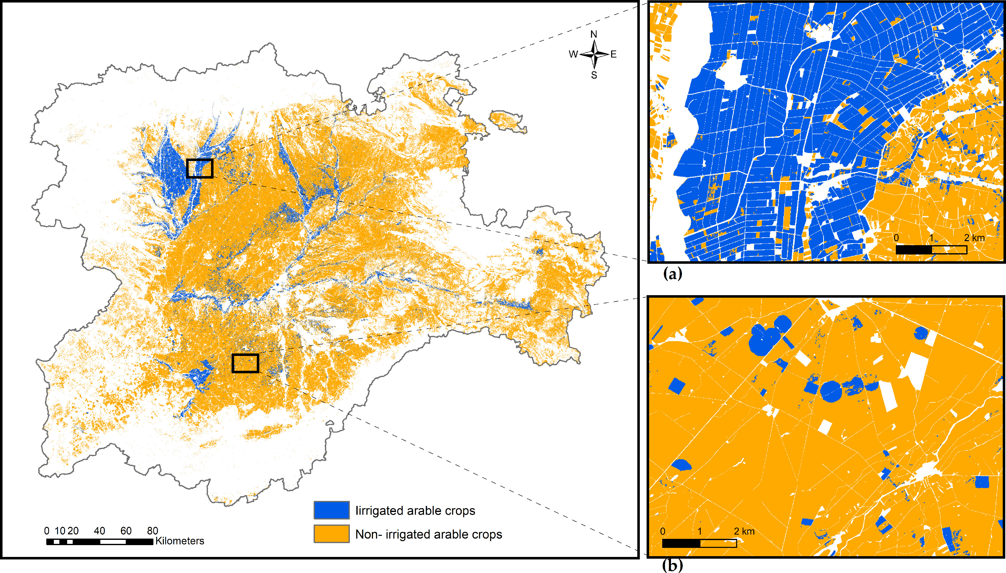
In this context, the PA of Castile and León (Spain) has been involved since the very beginning of the setting out of the new CAP monitoring approach, in 2018. Therefore, a new system of controls has been set to be applied to the main aid lines from the first pillar of the CAP in which irrigation is not a determining factor, such as basic payment subsidies (BPS) and its derivates, Young Farmers Scheme, Greening, and all Voluntary Coupled Support schemes. In all, it addressed eight first pillar schemes in 2019. This meant that in Castile and Leon over 5000 holdings covering almost 340,000 ha were checked by monitoring, which turned out that more than 63 million euros were paid to farmers in the phase-in area thanks to CbM. This first experiment was large enough to draw conclusions for next year.

Among other products and strategies, one of the key base information layers on which this system relies on is the Castile and Leon crops and natural land map (MCSNCyL, Spanish acronym) which is a land cover layer, updated twice a year, at the middle of the agricultural campaign, in July, and, at the end of the campaign, in October [2]. The project began in 2013, and since then, layers have been generated annually from 2011 to 2019. From 2017 on, this regional land cover map is generated with 10 m ground sampling distance (GSD) spatial resolution, thanks to the pair of satellites S-2A and S-2B of the constellation Sentinel within the Copernicus program. This spatial resolution is optimal for agricultural land monitoring since it has been reported that fine spatial resolutions of 10–30 m are ideal for regional-scale monitoring purposes [3]. Recently, there have been several studies proving its good performance of using Integrated Administrative Control System (IACS) data for crop type mapping [4]. There are other sources to extract the crop type information, such as the global ESA-CCI Land Cover product which distinguishes irrigated cropland or post-flooding areas [5]. Unfortunately, their spatial resolution is far from being convenient for this purpose since its spatial resolution of 300 m GSD is so coarse that it is ineffective for agricultural monitoring at parcel level. Using the ESA-CCI crop map to identify irrigation, most of the plots smaller than 9 ha would be ignored, which account for over 95% of all agricultural plots in Castile and León, where the average plot is 2.4 ha. Other global irrigation datasets are the United Nations Food and Agricultural Organization (FAO) and Rheinische Friedrich–Wilhelms–University deriving Global Map of Irrigation Areas version 5 [6] with a spatial resolution of 7 km in this area, and the Global Irrigated Areas Mapping from Institute Water Management Institute (IWMI) at 750 m spatial resolution [7].

In contrast, the MCSNCyL can detect plots greater than 0.01 ha, thus most of the plots in the region can be identified. The overall accuracy achieved and that obtained in each crop category considered in this crop map [8] were highly acceptable and enables it to be used in the crop identification to determine whether the declared crop was reliable or not. This has been demonstrated after the first experience using CbM in the region over the phase-in area. As an extra validation process, field visits were carried out to verify the grade of reliability and the result was also successful (not shown here) and proved that this regional crop map met some of the basic requirements for the CAP control system, such as crop type identification, agricultural activity control or crop diversification assessment.

However, following the EC regulations regards to phase-in period [1] the aids control system in Castile and León should gradually keep on developing towards the control aids in the second pillar of the CAP (rural development policy). This type of aids implies the need to establish a system that allows determining if the plots are actually irrigated since some of these lines establish limitations in relation to the use of water. In addition, the cross-compliance of the CAP (a set of basic rules that farmers must respect in order to receive EU income support), which until now has not been subject to monitoring controls, also implies that irrigation should be carried out only in plots that have rights to do so. Cross-compliance fulfillment control is expected to be addressed also in the near future. Thus, any support offered to the decision-making system in terms of irrigation identification is going to be an essential part of the Area Monitoring System with the current regulation and especially with the new CAP post-2020.

Thus, under this background, it is necessary to study and assess different methodological approaches to offer a product that distinguishes irrigated plots from the non-irrigated ones. To achieve this objective, in this study two strategies are presented, assessed, and discussed in order to offer a solution in the first place to our own PA, and in second place to the rest of the interested community, other PAs, and stakeholders.

The importance of the implementation of a methodology to detect irrigated crops also lies in the current limitation of knowing the cropland area actually irrigated [9], as well as its annual variation, particularly with regards to herbaceous or arable crops. Based on our experience in CAP controls, the data recorded in the farmers’ aid application forms are related mainly to the possibility to irrigate that parcel, regardless of the actual regimen of the current crop in the plot. For this reason, the study presented here provides information of great interest not only for the future CbM, but also for irrigation planning and modernization, crop yield statistics, and water management. The irrigated area estimation and identification of irrigated crops have been the subject of numerous research works [10,11,12] precisely because of the importance of having as much knowledge as possible of the use of water in an increasingly water-scarce world. Therefore, the ultimate goal to be achieved is to have a better understanding of the use of water for agriculture in our region and thus be able to achieve the objectives proposed by the European guidelines for more efficient agriculture and sustainable water resources.

Given the relevance of this issue, in the last decade, several studies have addressed this issue and have proposed different methodologies to map and monitoring irrigated areas using remote sensing data. Ambika et al. (2016) [11] developed annual irrigated area maps at a spatial resolution of 250 m for the period of 2000–2015 in India using the normalized difference vegetation index (NDVI) data from the moderate resolution imaging spectroradiometer (MODIS). Vogels et al. (2019) [13] proposed a methodology with a semi-automatic classification using image segmentation and variables such as shape, texture, neighbor, and location apart from commonly used spectral variables obtaining excellent results over a small area (669 km²), but requiring visual interpretation to label the training and validation dataset. The extent of our study area is 140 times larger than that, and visual interpretation is not feasible for operational classification over such a large area. More recently, there has been a plethora of works addressing this issue [13,14,15,16,17]. A special interest has been focusing on radar data, especially on Sentinel-1 or the synergy between Sentinel-1 and Sentinel-2 to propose more methodological approaches to detect irrigated areas [15,16,17].

However, what the checks by monitoring require is a methodology to assess the regular or continuous irrigation on a certain plot, or the probability of having been watered at some point during the development of the crop, by means of an automatic classification without any visual interpretation, since the vast extension we need to address it would be a very time-consuming data preparation process. Timing is a key point to consider if we want to check farmer’s applications on the ongoing agricultural campaign. Besides, the average size of an agricultural plot in Castile and León is about 2.4 ha, thus we need a resulting map with a fine spatial resolution over 20 m GSD to have a minimum quantity of pixels per plot, which also allows us to know its intra-parcel variability to let us detect no irrigation, homogeneous irrigation, or occasional irrigation.

Considering the above, in 2019 it was carried out a work to investigate if the traditional methodology employed to elaborate annually the MCSNCyL was also suitable to detect herbaceous irrigated crops. This research gave, as a result, a work presented in the Congress of the Spanish Association of Remote Sensing in 2019 [18]. In this work, the performance of the MCSNCyL approach for detecting irrigated agriculture was assessed obtaining very satisfactory accuracies. As examples, the ranges of F-score values obtained in the four irrigated crops with the most dedicated area in Castilla y León were (96.8–98.2), (62.7–77.8), (76.7–84.9), and (92.3–94.9), for maize, irrigated wheat, irrigated alfalfa, and sugar beet, respectively, during 2016, 2017, and 2018. Thus, it was proved that our method based on a decision tree algorithm and IACS data as reference data gave very accurate results for detecting irrigated agriculture over a national-scale area and even considering more than one hundred of land cover classes. It is reasonable to presume that, if the number of classes detected was decreased or the study area was smaller, the accuracy measures would be even higher. We also researched this assumption in 2019, but the results were never disseminated. That year, the CAP monitoring system designed in Castile and León was expected to check farmer’s applications in a phase-in area covering 8239 km², because our region was one of the 15 regions committed to carrying out the checks by monitoring from 2019 onwards. Thus, the same classification method was applied in the phase-in area, but only addressing 37 classes in order to improve the final accuracy. The overall accuracy and kappa index obtained were 94.60% and 0.93, respectively, in the phase-in area. Therefore, the MCSNCyL methodology with a reduced number of classes could meet the need for detecting irrigated cropland in order to support the checks by monitoring. However, this new approach of the traditional methodology would have a constrain regards to the minority crops that are not represented within the 37 classes directly derived from MCSNCyL 2019, and so, they will not be detected as irrigated, if necessary. That was the starting point to consider that it would be more convenient to get a binary classification map, where there were not land cover classes, but rather a pixel identification as irrigated or rainfed. That way, it would be possible to detect irrigated pixels in any land cover if full or partial watering had been applied. Ambika et al. (2016) [11] derived irrigated area maps according to agroecological zones using the NDVI threshold with satisfactory accuracies since Ozdogan, et al. (2008) [10] previously had demonstrated that the NDVI threshold approach was promising for identifying irrigated areas. Therefore, we consider including in the methodology a variable determining different agroclimatic areas in order to consider that crops show phenological differences depending on which agroclimatic area they are developed. We also include in both approaches the NDVI images on certain key dates.

Therefore, the main aim of this study is to present a new variant derived from the MCSNCyL methodology to obtain the regional crop map [18] which provides us with irrigated binary maps. This new approach uses the same classifier, reference data, and satellite images. The difference between them is the ancillary data and the classes definition. The reference data for irrigated crop maps will require to reclass the very detailed legend with more than one hundred classes to just two: irrigated or not irrigated class. The comparison of the results of the two variants of the same methodology (a land cover map of 121 classes versus a binary irrigation map) to detect irrigated crops in Castile and León will be analyzed to determine which one is more convenient to be implemented in the checks by monitoring in the phase-in area of Castile and Leon. Besides, a detailed implementation methodology to include the irrigated binary maps results into the CAP monitoring system will be described in order to let it be operational in this ongoing year 2020.

2. Materials and Methods

2.1. Different Methodological Strategies Tested

As was mentioned in the introduction, in this study two approaches derived from the same methodology [2,18] are tested to assess the irrigation in each declared plot by farmers in the CAP subsidy application.

• High detailed thematic map (HDTM) including irrigated and/or rainfed crop classes: It distinguishes 121 land cover classes, including 45 specific crop types. The list and descriptions of these classes can be found in

  Table A3. List of the 121 classes distinguished in the High Detailed Thematic Map (HDTM) grouped by the type of coverage to which they belong. The percentages in the forest classes indicates tree density: very sparse (10–40%), sparse (40–70%), and thick (>70%).

  Class Description Grouped by Coverage Type
  Rainfed Arable Crops:	Irrigated Arable Crops:
  Wheat	Maize
  Barley	Sorghum
  Rye	Bean
  Oats	Irrigated wheat
  Triticale	Irrigated barley
  Fallow	Irrigated alfalfa
  Sunflower	Irrigated sunflower
  Rapeseed	Irrigated rapeseed
  Green peas	Irrigated rye
  Lumps	Irrigated oats
  Chickpeas	Irrigated triticale
  Lentils	Sugar beet
  Vetch	Potatoes
  Ervils	Poppy
  Alfalfa	Strawberries
  Other forage crops	Pumpkin
  Esparceta	Garlic
  Raygrass	Onion
  Lathyrus cicera	Carrot
  Locust beans	Leek
  Other land cover areas:	Horticultural crops
  Artificial and Urban areas	Permanent crops:
  Rocky areas	Vineyard
  Waterbodies	Olive groves
  Natural and Semi-natural vegetation:	Almond trees
  Mesoxerphytic basophilic grasslands	Peaches trees
  Southwestern Mediterranean perennial and Iberian summer pastures	Forest Areas:
  Rushes	Pinus sylvestris (>70%)
  Weed and subnitrophilous grass and crucifer communities	Pinus sylvestris (40–70%)
  Gullies	Pinus sylvestris (10–40%)
  Nardus grasslands and other non-cryoturbed pastures of the high mountain	Pinus nigra (>70%)
  Mesophyll basophilic grasslands	Pinus nigra (40–70%)
  Nardus grasslands of the High mountain	Pinus pinaster (>70%)
  Subalpine cryoturbated-soils grasslands	Pinus pinaster (40–70%)
  Atlantic and sub-Atlantic lowland and submontane hay meadows	Pinus pinaster (10–40%)
  Rosemary (Rosmarinus officinalis)	Pinus pinea (>70%)
  Gipsophilic bush	Pinus pinea (40–70%)
  Lavender (Lavandula stoechas)	Pinus halepensis (>40%)
  Mixed thyme	Pinus radiate (>70%)
  Grassy dwarf-shrub garrigues	Pinus radiata (40–70%)
  Thymes-dried grass	Juniperus thurifera (>40%)
  Silicaphillic scrubland with creeping juniper	Juniperus thurifera (10–40%)
  Basophilic juniper field (Juniperus communis) and/or Juniperus thurifera	Quercus ilex (>70%)
  Gorse (Genista sp.).	Quercus ilex (40–70%)
  Hedgehog-heaths dominated by Genista hispanica	Quercus ilex (10–40%)
  Hedgehog-heaths dominated by Erinacea anthyllis or Genista pumila cushion	Quercus faginea (>70%)
  Echinospartum dominated hedgehog-heaths and Genista and Astragalus heaths	Quercus faginea (40–70%)
  Gorse thickets of Ulex spp.	Quercus faginea (10–40%)
  Whiteleaved rock roses	Quercus pyrenaica (40–70%)
  Gum rock roses	Quercus pyrenaica (>70%)
  Cytisus purgans piornal	Quercus pyrenaica (10–40%)
  High mountain Genista piornal	Fagus sylvatica (>70%)
  Open formations with Cytisus scoparius	Populus plantation (40–70%)
  White-flowered broom fields (Cytisus multiflorus) and related	Populus plantation (10–40%)
  Deciduous thorny forest	Eucalyptus camaldulensis (40–70%)
  Juniperus phoenicea scrub	Eucalyptus camaldulensis (>70%)
  Juniperus scrub	Eucalyptus globulus (>70%)
  Hydrophilic heaths	Populus plantation (>70%)
  High thick heaths	Quercus rubber (>70%)
  Low thick heaths	Quercus rubber (40–70%)
  Low sparse heaths	Castanea sativa (>70%)
  Heaths-rock roses (Cistus ladanifer)	Castanea sativa (40–70%)
  Bearberry	Pinus sylvestris (>70%)

  of Appendix A.
• Irrigation binary map (IBM): This map only has two categories showing irrigated or non-irrigated pixels.

The core of the methodology used is based on the US crop data layer [19] and the US National Land Cover Database (NLCD). This product takes advantage of supervised classification systems based on machine learning algorithms with huge amounts of satellite images. Machine learning allows computers to become more accurate in predicting outcomes without explicit programming, using algorithms that iteratively learn from data. At its core, machine learning is the process of automatically discovering patterns in data. In particular, the decision trees algorithm used here has proved to be efficient for land cover classification [20]. This methodology [19] originated the MCSNCyL project [2] which is a dynamic and public operational service since 2013 that produces a land cover layer twice a year, a provisional version in July and a definitive and more accurate version at the end of each year. All annual products generated from 2011 are published on the ITACyL website [2] where a data viewer exists to retrieve the information and to allow the download printable high-resolution maps and the raw data to let expert users handle these data.

2.2. Study Area

The study area covers the whole region of Castile and León (Spain). This region is in southern Europe (Figure 1a) and has an extent of 94,224 km², representing one fifth of the total area of Spain. It consists mainly of a dry and wide basin defined by the Duero river and its contributors with an average altitude of 800 m, surrounded by mountains.

The territory is composed mainly of areas of extensive herbaceous crops or natural vegetation. Most of the arable land (55,000 km²) is located in the center of the basin (Figure 1b), where rain averages 500 mm per year. Dryland farming is based in winter crops such as cereals, namely wheat or barley, and also forage. Ten percent of the arable land is irrigated in summer with water stored in reservoirs. The main irrigated crops are maize, barley, wheat, sugar beet, alfalfa, and potato. Among permanent crops, vineyards are the most important.

2.3. Data

The data sources have been divided into three groups: Satellite images, representing the core of the independent variables in the machine learning for both strategies, NDVI images, and ancillary data which are different in each approach.

2.3.1. Satellite Imagery

The Copernicus program of the EC with its implementation of a free and open access policy for the Sentinel data provides an excellent opportunity for the scientific community and public administration to develop a plethora of products to support them in a lot of issues. Specifically, the fine spatial resolution of the Sentinel-2 optical sensors ranging from 10 to 60 m and its 5 days revisit time with Sentinel 2A and 2B satellites combined, allow us to generate land cover maps with 10m GSD. Sentinel-2A and Sentinel-2B are a constellation of two identical optical sensors with 13 spectral bands. The Sentinel-2 images used in this work are the Level-2A products that are atmospherically corrected using Sen2Cor processor and provide bottom of atmosphere (BOA) reflectance in cartographic geometry. These products are currently processed by ESA and have been downloaded from the Copernicus Open Access Hub (https://scihub.copernicus.eu/).

Processing large amounts of images such as the Sentinel-2 archive is a computationally demanding task. The European Space Agency (ESA) provides the Sentinel-2 L2A images in 100 × 100 km tiles. There are three Sentinel-2 orbits: R037, R137, and R094 containing 33 tiles covering the Castile and Leon region (Figure 2). The total amount of available images covering the whole study area from January 2019 until September 2019 was 1797 tiles, although only approximately 50% of them were completely downloaded, accounting for over 1.5 TB of data used in the study.

Table 1. Sentinel-2A and Sentinel-2B images available and downloaded covering the study area.

Relative Orbit	Tiles Covering CyL	Total Tiles Available	Tiles Downloaded
R037	10	540	290
R094	8	432	192
R137	15	825	420
Total	33	1797	902

summarizes the orbit and number of tiles used in this study

Due to the large extension of the study area, we opt for creating relatively cloud-free images composite of each orbit and date instead of a composite with tiles from the 3 orbits and different dates. The selection criteria for optimal images to create the composites were based on the analysis of the metadata of all the granules that cover the study area in each orbit. When most of the tiles included in each orbit and day have less than 25% cloud cover, the tiles are downloaded and the composite is generated. Due to the need to have images over the whole region covering the period of maximum interest of all crops in order to facilitate their classification, some image composite per orbit may slightly exceed the cloud cover threshold established by including granules with more clouds than desired.

For this study, 81 Sentinel-2 tiles composite per orbit and day images were processed, 40 from Sentinel-2A and 41 from Sentinel-2B. The selection of the bands was carried out one year before by means of a sensibility analysis of different band combinations and the accuracy of the resulting land cover map considering all land cover classes (more than one hundred). The relevance of each band as an independent variable in the classifier was determined by assessing the resulting files of the See 5 Classifier process, where there is information letting us know how each individual band contributes to the classifier. Thus, a multiband image with 6 bands (B2-B4-B8-B5-B11-B12) was generated after processing each original L2A Sentinel image. The spectral region of blue, red, and near-infrared (NIR) corresponding to bands B2 (490 nm), B4 (665 nm), and B8 (842 nm) have a spatial resolution of 10 m but the spectral bands B5 (705 nm), B11 (1910 nm), and B12 (2190 nm) have 20 m, corresponding to red-edge and shortwave-infrared (SWIR1 and SWIR2) respectively. As the final maps to be generated will be at 10 m GSD, a pan-sharpening process using a Geospatial Data Abstraction Library (GDAL) script, in particular a bilinear resampling (gdal_pansharpen.py), was applied to the 20 m bands to convert them into 10 m. First, we created a reference image from the 10 m bands B04 and B08, to use it as it was a panchromatic band. Afterward, we resampled the 20 m bands to 10 m on the basis of this previously created reference image. Note that only the 20 m bands B05, B11, and B12 are used in this study.

Concerning the number of images, as a rule of thumb, we recommend disposing of at least one cloud-free image per month for every orbit composite to be included. That way, we were able to have enough spectral information to detect the phenological changes in the crops during the agricultural campaign.

NDVI Images

Numerous studies have included vegetation indexes into land cover classification [4,10,11,13,14,15,16,17,21]. Regarding the detection of irrigated crops and areas, six NDVI composite images have been created to be included as independent variables in the classifier. NDVI images were computed using the GDAL script (gdal_calc.py) from the 10 m Sentinel-2 bands B04 and B08. Actually, two relevant dates to distinguish irrigated crops in our region have been carefully selected according to the orbit composite availability and that the three selected orbit composites for the same date were cloud-free. The dates of the images selected are shown in

Table 2. Dates of the NDVI (Normalized Difference Vegetation Index) mosaicked images generated.

	R037	R137	R094
Middle growing season	26 March 2019	23 March 2019	30 March 2019
Ending growing season	30 May 2019	1 June 2019	3 June 2019

. The first date had to be around the end of March and the second date at the beginning of June. With both NDVI dates the differences given in the NDVI peak value in winter crops irrigated and non-irrigated are evidenced, as illustrated in Figure 3 where the histogram of NDVI values of irrigated pixels are compared to rainfed pixels in the R137 orbit image on two different dates, 23th March and 1st June, for two representative crops in the region, barley and alfalfa. The summer crops in our region are mostly or even exclusively cultivated in irrigation regime. Besides, in the first approach, six out of the seven crop classes with irrigation discrimination are winter crops, except sunflower.

2.3.2. Ancillary Data

Besides satellite imagery, it is possible and advisable to include more ancillary data in order to aid the classification algorithm to determine the class properly. These datasets constitute a complement and most of them might be available with the pan-European Copernicus land services. These data are considered very stable and therefore could be used for the ongoing year. However, since we have access to a lot of regional datasets with high-quality and updated information, we do not need to use external sources.

We used the following complementary data in the first approach to generate the HDTM:

• Land cover class information from Spanish Land Parcel Information System (LPIS) for each ongoing year.
• Digital Elevation Model (DEM) and its derivate Slopes and Aspect.
• Averaged precipitation map (over the last 30-year period, 1981–2010).
• Vegetation height and canopy cover fraction layers derived from LIDAR (Light detection and ranging). This dataset is available at the local level and improves considerably in the forest and natural vegetation discrimination. Therefore, for crop class discrimination, it is complementary but absolutely dispensable.

On the other hand, the following ancillary data are employed to derive the IBM:

• Regional crops and natural land map for the studied year, in this case, the MCSNCyL of 2019 [2].
• Castile and León agroclimatic zoning derived from 3 variables related to accumulated precipitation at key periods of phenological development of winter and summer crops, that is, in spring and summer, and with the average temperature of the warmest month. Four different zones have been obtained, zones with a value equal to 1, those with the highest precipitation in spring and summer and milder temperatures during July, and zones with a value of 4 that receive less precipitation and have higher temperatures during July.

2.3.3. Reference Data

IACS database containing CAP farmers’ applications is the keystone from which we obtain the reference data for our crop classification system. From 2017 on, the farmers make their application claims by means of the Geo-Spatial Aid Application (GSAA) allowing the administration to get directly the geographical features with alphanumerical associated information. This database is compiled by the local PA and contains an invaluable source of training cases for crop identification due to the degree of detail and the truth contained in farmers’ applications regarding the declared crop. Thus, this database is a perfect reference dataset for a crop map classification. GSAA also includes an attribute about the nature of the water availability (irrigated or rainfed) in the parcel. This data could be considered more as an attribute regarding the right to use the water than an actual sign of water allocation within the parcel during that campaign.

The GSAA is the geographical farmer’s declaration based on cadastral references, which means that these GSAA does not fit exactly with the agricultural plots. Thus, from these GSAA containing the required crop type information, a preprocessing has been done to merge those GSAA belonging to the same holding and declaring the same crop. That way, we work with minimum management units as similar as possible to the agricultural parcels on the land. These new entities are the features of interest (FOIs) and are the reference data where the training cases are extracted from.

Concerning irrigated crops, rigorous filtering from all FOIs declared has been done in order to select the most reliable training cases. This selection is carried out thanks to two complementary sources of information, the Spanish LPIS (SIGPAC) and a shapefile of irrigation districts provided by the Spanish part of the Duero River Basin Authority. LPIS provides us information about the irrigation coefficient (IC) of each parcel ranging from 0% to 100%, meaning the percentage of the plot that is actually irrigated. The vectorial layer of irrigation districts tells us what areas have good infrastructure and cheap water allocation. This only implies that a crop cultivated there is more likely to be irrigated but not that it was actually irrigated. On one hand, we assure that all FOIs declared as irrigated for the CAP subsidies are actually irrigated when they have been assigned an IC of 100% and are located within an irrigation district. As opposed, concerning the selection of rainfed crop training cases, only those with an IC of 0% were candidates. Besides, we only select those plots located at least 2 km away from an irrigable area to make sure that the parcels are more likely to be without irrigation structures.

Regarding natural and semi-natural land cover cases, they have been provided by regional public administration responsible for natural resources management and control (Dirección General del Medio Natural). As for forest types they rely on two data sources: the Spanish National Forest Inventory plots (except for Populus spp., Pinus radiata, Eucalyptus spp., Castanea sativa, and Quercus robur, for which we have generated training datasets manually with aerial photography and ancillary information), and LIDAR data.

In the first highly detailed regional land cover layer obtained, there are seven crop classes that can appear in both regimes, irrigation and rainfed. The remaining of the crop classes can only be presented in one of the systems either irrigated or rainfed. For training cases in the binary classification, the latter reference data were reclassified into just two categories, irrigated or not irrigated.

2.4. Classification Algorithm

The classification has been performed using a pixel-based approach. This classification is carried out by using the data-mining tool C5.0, distributed freely under the GNU General Public License (GPL) [22]. This C5.0 is an improvement on the previous C4.5 algorithm used to generate decision trees from a set of reference data.

Before using this algorithm, it is necessary to randomly sample the reference data to obtain the training pixels on which the creation of decision trees will be based on. This step has been done with the NLCD sampling tool implemented in ERDAS imagine 2018 [23]. By this tool, we select a random and stratified sample from the reference dataset that will be the training cases and set aside a smaller sample of the remaining reference data to validate internally the decision tree creation process. The amount or percentage of cases/pixels used by the algorithm and the internal test cases are predefined by the user in the NLCD tool. In this study, we set 560,000 cases for training the classifier and 240,000 for internal validation of the model, establishing a minimum number of samples per class to 2000 cases. Afterward, the algorithm C5.0 is run on a Linux terminal and needs to set some parameters before being run in order to customize the process of decision tree creation. The setting is established to acquire a boosted classifier using tests that require two branches with at least two cases implied and with a pruning confidence level of 25% preventing the overfitting of the decision tree learning algorithm. Once this step is finished, the final generated decision trees are applied to all pixels of every satellite images and ancillary data, obtaining the land cover classification of the whole region in a unique step. The final image classification using the previously created decision trees has been done using the See Classifier tool of the NLCD plugin incorporated in ERDAS.

Postprocessing

Normally several postprocessing steps take place after classification in order to provide a more easily interpretable map: simplify (grouping) the mapped classes if required due to accuracy problems and crop identification requirements and elimination of speckle artifacts, or the “salt and pepper,” an effect common to pixel-based classifications of fine spatial resolution imagery. The procedure is carried out using the sieve command from GDAL. For this study, the original version without grouping has been issued for the highly detailed land cover map in order to assess the ability to detect irrigated croplands versus the irrigation binary maps.

2.5. Classification Accuracy Assessment

In order to assess the performance of the two approaches studied in this work and to have some knowledge about how much confidence each one provides, the same dataset is required for the validation process of both approaches. This dataset belongs to the same reference data gathered from IACS data, the only caveat being that it must not be involved in the learning process of the classifier. Therefore, the training cases used for the classifier were discarded from the reference data, keeping the rest of the data for validation. The resulting validation dataset covers over a million hectares, which comprises over 10% of the whole region and almost 30% of the total arable cropland in Castile and Leon. The nature of both approaches implies that the validation dataset should be postprocessing to be able to validate the irrigated crop map. Thus, a reclassification process will be needed to make it usable to validate the irrigation binary maps. Afterward, an independent validation was done by comparing the predicted crop types or category (irrigated/non-irrigated in the case of binary maps) with the known crops (or category) using the validation dataset. This validation process has been carried out employing the module r.kappa [24] including in Geographical Resources Analysis Support System (GRASS) which is a free and open-source geographic information system (GIS) software suitable for advanced management and analysis of geospatial data under the GNU GPL. This module r.kappa computes the confusion matrix and returns accuracy measures obtained of pixel-based classification in a plain text file, such as kappa coefficient [21,25] for overall and each class and commission errors, a complement of the user’s accuracy (UA), and omission errors, a complement of the producer’s accuracy (PA). UA (also called precision) evaluates how well the predicted crops agree with the known reference data (i.e., the IACS field data), while PA (also called recall) measures the agreement between the reference data and the prediction [4]. OA assesses the overall performance of a model and is the ratio of correctly predicted crops and the total number of predicted crops. We also compute the widely used F-score, which is the harmonic mean of UA and PA.

The assessment of the high detailed thematic map with 121 classes brings us also class-specific metrics. However, this map will be converted into a binary classification through a reclassification process so that the results of both strategies are analogous and comparable. In the context of evaluating the precision of a binary classification with unbalanced classes (more rainfed pixels than irrigated pixels in our case), a more suitable alternative metric has recently been proposed for these cases, the Matthews correlation coefficient (MCC) [26]. It might be useful to consider the normalized MCC, defined as nMCC (see

Table 3. Summary of the confusion matrix obtained and other accuracy measures adopted.

	Reference Data
Class Mapped	1	2	Row Sum
1	TP *	FP *	$TP+FP$	Precision/UA * $TP/TP+FP$
2	FN *	TN *	$FN+TN$
Col Sum	$TP+FN$	$FP+TN$	$TP+FP+FN+TN$
	Recall/PA * Sensitivity $TP/TP+FN$	Specificity $TN/FP+TN$		Overall Accuracy $TP+TN/TP+FP+FN+TN$
		F1 score $2\times Precision\times Recall/Precision+Recall$
nMCC $MCC+1/2$		Matthews correlation coefficient (MCC) $TP\times TN-FP\times FN/\surd \left(TP+FP\right)\left(TP+FN\right)\left(TN+FP\right)\left(TN+FN\right)$

* TP = True Positives; FP = False Positives; FN = False Negatives; TN = True Negatives; UA = User’s Accuracy; PA = Producer’s Accuracy

), and linearly projecting the original range into the interval [0,1], being value 0.5 the average value for the coin-tossing classifier, and 1 for perfect classifiers. Using this latter measure, all metrics computed are comparable among them. All the accuracy metrics calculated are depicted in Table 3.

2.6. Implementing Process in the CAP Monitoring System

As was previously explained, the shift of the CAP controls towards the new paradigm of CbM means that every parcel that claims any CAP subsidy has to be monitored and assessed in terms of agriculture activity evidence [1]. Within the CbM framework, the concept of Marker has been adopted. A Marker is a binary state of the monitored parcel that informs whether a certain requirement for a subsidiary schema is accomplished or not. The combination of two or several markers allows the CAP control system to make a judgment on the compliance of the parcel for that schema. In this sense, the binary irrigation map generated in this work along with the S2 NDVI series and the MCSNCyL [2], might be very useful to characterize a parcel in terms of decision about presence/absence of crop, compatible vegetation development with the declared crop, or even irrigation/no-irrigation activity as a novelty this year.

Besides the information derived from EO data, to perform the above-mentioned judgment, the CAP control system needs the boundaries of the parcel in vector format which are provided by the FOIs previously created along with the declared crop in the GSAA. Once all the FOIs within the region boundaries (2,126,124) are inserted into the CAP control system database, all of them will be intersected with the irrigation map selected as the best strategy. Several scripts in python programing language have been developed to carry out the extraction of all this information and populate the CAP control system database. The scripts made intensive use of specific libraries for geospatial information managing such as gdal, rasterio, shapely, and fiona. Other libraries were also needed to compute some statistics, these mainly were numpy, scipy, and pandas. Apart from the libraries themselves, the scripts were developed to take advantage of all the available computer resources by distributing the process over all the processors in the machine and to avoid memory overload that could lead to a reduction in the performance.

In regards to the aim of creating a specific irrigation-based marker for each FOI, the information required is going to be collected from the irrigation identification map proposed in this work. Basically, it is the count of pixels belonging to each class (irrigated/non-irrigated) within the boundaries of each FOI and the percentage that it represents over the overall counting. So, some conclusions are gathered about the potential of its use on a regional scale. Nonetheless, the final decision to be made in the aid control system on whether or not a parcel is detected as irrigated using this irrigated binary map will require further analysis. A certain threshold could be set for each crop, after which each plot will be considered irrigated only if it exceeds that percentage of pixels detected as irrigated. As an example, a table will show the percentage of plots of each declared crop that will be considered irrigated depending on the threshold that was established. Nevertheless, the application of that threshold might imply that an aid application was proposed to be amended by the farmer, therefore how this decision should be taken by the competent authority is out of the scope of this study. This work just focuses on proposing a tool to ease for them this complex final decision, in which more factors, such as economical issue, might play a key role.

3. Results

3.1. Assessment of the HDTM: Highly Detailed Thematic Map Including Irrigation Discrimination

The overall accuracy obtained in the first approach (HDTM) was 87.13% and a kappa coefficient of 0.85 (see Appendix A

Table A1. Class-specific accuracy measures obtained after validation of the land cover map with high thematic detail (HDTM of 121 classes) distinguishing irrigated arable crops from rainfed arable crops and permanent crops, over the whole region of Castile and Leon. Natural and semi-natural vegetation and other coverages are not shown here for sake of brevity.

Land Cover Type	Class Description	CI * User’s Accuracy	Comission. Error (%)	CI * Producer’s Accuracy	Omission Error (%)	F-Score	Kappa
Rainfed Arable Crops	Wheat	84.77 ± 0.12	15.23	92.29 ± 0.09	7.71	88.37	0.80
	Barley	89.39 ± 0.1	10.61	93.56 ± 0.08	6.44	91.43	0.86
	Rye	83.01 ± 0.42	16.99	58.19 ± 0.46	41.81	68.42	0.82
	Oats	71.16 ± 0.43	28.84	59.45 ± 0.43	40.55	64.78	0.70
	Triticale	85.86 ± 1.15	14.14	22.58 ± 0.71	77.42	35.75	0.86
	Fallow	86.47 ± 0.15	13.53	94.28 ± 0.1	5.72	90.21	0.84
	Sunflower	92.3 ± 0.15	7.70	90.32 ± 0.17	9.68	91.30	0.92
	Rapeseed	95.99 ± 0.63	4.01	65.92 ± 1.27	34.08	78.16	0.96
	Green peas	78.69 ± 0.58	21.31	76.9 ± 0.59	23.10	77.79	0.78
	Lumps	45.88 ± 5.56	54.12	93.37 ± 3.96	6.63	61.53	0.46
	Chickpeas	82.89 ± 1.22	17.11	64.73 ± 1.37	35.27	72.69	0.83
	Lentils	84.67 ± 1.02	15.33	72.09 ± 1.17	27.91	77.87	0.85
	Vetch	76.06 ± 0.39	23.94	75.2 ± 0.4	24.80	75.63	0.75
	Ervils	84.82 ± 1.5	15.18	46.93 ± 1.55	53.07	60.42	0.85
	Alfalfa	88.4 ± 0.36	11.60	84 ± 0.4	16.00	86.14	0.88
	Other forage crops	75.47 ± 1.37	24.53	33.34 ± 1	66.66	46.25	0.75
	Esparceta	81.38 ± 1.66	18.62	52.41 ± 1.7	47.59	63.76	0.81
	Raygrass	77.01 ± 1.34	22.99	47.11 ± 1.24	52.89	58.46	0.77
	Lathyrus cicera	72.62 ± 1.83	27.38	55.96 ± 1.78	44.04	63.21	0.73
	Locust beans	54.38 ± 2.67	45.62	74.18 ± 2.74	25.82	62.76	0.54
Irrigated Arable Crops	Maize	98.92 ± 0.09	1.08	98.98 ± 0.09	1.02	98.95	0.99
	Sorghum	40.99 ± 8.58	59.01	95.06 ± 5.76	4.94	57.28	0.41
	Bean	21.72 ± 11.16	78.28	97.77 ± 8.49	2.23	35.54	0.22
	Irrigated wheat	90.09 ± 0.42	9.91	79.01 ± 0.54	20.99	84.18	0.90
	Irrigated barley	89.01 ± 0.79	10.99	47.86 ± 0.93	52.14	62.25	0.89
	Irrigated alfalfa	92 ± 0.54	8.00	88.99 ± 0.62	11.01	90.47	0.92
	Irrigated sunflower	92.12 ± 0.75	7.88	63.87 ± 1.12	36.13	75.44	0.92
	Irrigated rapeseed	87.69 ± 2.11	12.31	95.01 ± 1.46	4.99	91.20	0.88
	Irrigated rye	72.43 ± 3.44	27.57	79.45 ± 3.26	20.55	75.77	0.72
	Irrigated oats	83.42 ± 1.93	16.58	63.94 ± 2.18	36.06	72.40	0.83
	Irrigated triticale	53.27 ± 4.24	46.73	85.12 ± 3.82	14.88	65.53	0.53
	Sugar beet	97.56 ± 0.45	2.44	93.66 ± 0.7	6.34	95.57	0.98
	Potatoes	92.07 ± 1.01	7.93	92 ± 1.01	8.00	92.03	0.92
	Poppy	76.24 ± 5.12	23.76	98.49 ± 1.67	1.51	85.95	0.76
	Strawberries	84.73 ± 3.17	15.27	95.78 ± 1.88	4.22	89.92	0.85
	Pumpkin	69.1 ± 8.08	30.90	95.38 ± 4.31	4.62	80.14	0.69
	Garlic	66.23 ± 3.62	33.77	94.27 ± 2.12	5.73	77.80	0.66
	Onion	73.72 ± 3.57	26.28	92.93 ± 2.34	7.07	82.22	0.74
	Carrot	73.08 ± 3.38	26.92	91.67 ± 2.36	8.33	81.33	0.73
	Leek	54.92 ± 5.92	45.08	95.72 ± 3.18	4.28	69.80	0.55
	Horticultural crops	68.54 ± 5.96	31.46	85.57 ± 5.04	14.43	76.11	0.69
Permanent crops	Vineyard	99.2 ± 0.16	0.80	94.11 ± 0.42	5.89	96.58	0.99
	Olive groves	99.14 ± 0.64	0.86	99 ± 0.69	1.00	99.07	0.99
	Almond trees	97.08 ± 1.03	2.92	82.25 ± 2.16	17.75	89.05	0.97
	Peaches trees	69.67 ± 9.27	30.33	99.28 ± 2.04	0.72	81.88	0.70
		Overall accuracy (%)				87.13
		Kappa index				0.85

* CI: Confidence Interval of the estimate for a 95% confidence level.

) considering a great number of land cover classes, 121 land cover classes, including 44 crops: 19 rainfed arable crops, 21 irrigated arable crops, and 4 permanent crops. For the sake of a better visualization in Figure 4 the classes are depicted grouped into the main land cover types.

The two more representative crop classes within the region are by far wheat and barley (see Appendix A

Table A2. Area covered (hectares) by each class in the classified map, reference data, training data and validation data in the first classification approach (HDTM of 121 classes) in the entire region of Castile and León. Non-crop classes are not shown here for sake of brevity.

Land Cover Type	Class Description	Map Area (%)	Map Area (ha)	Ref. Data (%)	Ref. Data (ha)	Train. Data (ha)	Validat. Data (ha)
Rainfed Arable Crops	Wheat	10.02	943,829	22.26	307,148	1245	305,903
	Barley	9.21	868,332	23.67	326,642	1324	325,318
	Rye	0.89	84,174	3.16	43,605	177	43,428
	Oats	1.37	129,485	3.67	50,656	205	50,451
	Triticale	0.07	6357	0.97	13,354	54	13,300
	Fallow	8.67	816,624	13.82	190,718	773	189,945
	Sunflower	3.02	284,781	8.82	121,773	494	121,279
	Rapeseed	0.12	11,712	0.39	5388	22	5366
	Green peas	0.45	42,481	1.42	19,563	79	19,484
	Lumps	0.01	851	0.01	172	20	152
	Chickpeas	0.08	7803	0.34	4670	20	4650
	Lentils	0.09	8478	0.41	5704	23	5681
	Vetch	1.13	106,821	3.33	45,962	186	45,776
	Ervils	0.04	3770	0.29	4004	20	3984
	Alfalfa	0.82	77,531	2.39	32,933	133	32,800
	Other forage crops	0.08	7928	0.62	8570	35	8535
	Esparceta	0.06	6084	0.24	3320	20	3300
	Raygrass	0.22	20,584	0.45	6260	25	6234
	Lathyrus cicera	0.05	4714	0.22	2993	20	2973
	Locust beans	0.03	2557	0.07	1001	20	981
Irrigated Arable Crops	Maize	1.44	136,100	3.90	53,857	218	53,639
	Sorghum	0.01	877	0.00	74	20	54
	Bean	0.01	518	0.00	32	20	12
	Irrigated wheat	0.63	59,301	1.59	22,005	89	21,916
	Irrigated barley	0.23	21,923	0.81	11,114	45	11,069
	Irrigated alfalfa	0.40	37,573	0.72	9884	40	9844
	Irrigated sunflower	0.16	15,271	0.52	7144	29	7115
	Irrigated rapeseed	0.05	4617	0.06	879	20	859
	Irrigated rye	0.07	6475	0.04	611	20	591
	Irrigated oat	0.05	4430	0.14	1886	20	1866
	Irrigated triticale	0.03	2702	0.02	353	20	333
	Sugar beet	0.22	21,003	0.34	4675	20	4655
	Potatoes	0.19	18,250	0.20	2772	20	2752
	Poppy	0.02	1918	0.01	225	20	205
	Strawberries	0.03	2640	0.03	458	20	438
	Pumpkin	0.01	727	0.01	111	20	91
	Garlic	0.03	2525	0.03	482	20	462
	Onion	0.03	2990	0.03	483	20	463
	Carrot	0.05	4912	0.04	547	20	527
	Leek	0.02	1562	0.01	176	20	156
	Horticultural crops	0.03	2902	0.01	207	20	187
Permanent crops	Vineyard	0.92	86,246	0.88	12,164	49	12,115
	Olive groves	0.12	10,972	0.06	812	20	792
	Almond trees	0.10	9087	0.09	1223	20	1203
	Peaches trees	0.20	18,487	0.00	86	20	66
	Total	100.00	9,422,714	100.00	1,381,745	7356	1,374,389

), representing more than half of the arable land of Castile and León. Both winter cereals obtained high-performance measures, an F-Score of 88.4 and 91.4, respectively, even though both are very similar botanically and the phenology and life cycle of the two species were basically similar. This is one of the key achievements of this map version since, in most of the published works with crop types classification, there is not a distinction between these two similar types of cereal [21,27] which are so important in a cereal area, such as Castile and León. Another milestone achieved in this approach is to be able to separate irrigated wheat and irrigated barley as well as independent classes, among others, reached acceptable accuracies, F-score of 84.8 and 62.3, respectively. However, it is worthy to highlight that there is misclassification among winter cereals are due to the same reason, for the similar botanic characteristics and phenology. In fact, it can be observed that all the winter cereals (wheat, barley, rye, oats, and triticale) in the classified map account for around 90–98% of all the training cases for these classes. Likewise, the summer cereals, maize and sorgo (this being a very minor cereal in our region) can be misclassified mainly between them because they are the most similar to each other. We have not seen that these errors are concentrated in any specific area. The errors are spatially distributed equally over the region.

In order to compare both strategies, the HDTM is reclassified into an irrigated/non-irrigated binary map. The irrigated class comes from all irrigated herbaceous crops (21 classes) and the rest of crops are labeled as non-irrigated. The accuracy measures of this layer are shown in

Table 4. Contingency table of the validation of the Highly Detailed Thematic Map (HDTM) reclassified as an irrigation binary map at pixel level.

	Reference Data
Class mapped	Irrigated	Non-irrigated	Row Sum	Precision
Irrigated	10,484,519	231,762	10,716,281	0.9784
Non-irrigated	1,247,632	88,622,758	89,870,390
Col Sum	11,732,151	88,854,520	100,586,671
Recall	0.8937		F1 score	0.9341
Overall Accuracy	98.53%		MCC	0.9270
Kappa	0.9258		nMCC	0.9635

. After the reclassification process, the validation provides a significant improvement in the overall accuracy comparing to the very detailed land cover map due to the drastic reduction of the number of classes. OA, kappa index and F-score were 98.53%, 0.9258 and 0.9341 respectively. As was previously explained, we also compute the normalized Matthews correlation coefficient (nMCC) which is more convenient for binary classification with unbalanced classes as is our case, with a higher percentage of non-irrigated areas than irrigated. The nMCC reached a value of 0.9635.

3.2. Assessment of the IBM: Irrigation Binary Map

Figure 5 depicts the IBM generated by the second approach, where it is possible to identify the main irrigation areas in Castile and León due to the fact that most of the detected irrigation fields are concentrated in those areas (Figure 5a). Otherwise, Figure 5b shows an area dominated by rainfed agriculture, where some pivots can be identified with a regular irrigation system.

The OA, kappa index, and F-score obtained in the binary approach (IBM) were 98.47%, 0.9228, and 0.9314, respectively. The normalized MCC was 0.9621 (

Table 5. Contingency table of the validation of the IBM.

	Reference Data
Class mapped	Irrigated	Non-irrigated	Row Sum	Precision
Irrigated	10,428,685	232,623	10,661,308	0.9782
Non-irrigated	1,303,466	88,621,897	89,925,363
Col Sum	11,732,151	88,854,520	100,586,671
Recall	0.8889		F1 score	0.9314
Overall Accuracy	98.47%		MCC	0.9242
Kappa	0.9228		nMCC	0.9621

). There is no significant difference with the results obtained by the HDTM. Therefore, on the basis of these accuracy measures, both maps would be sufficient enough to detect the main irrigated plots in Castile and Leon. However, as it will be explained later in the Discussion section, the IBM will be eventually chosen by addressing the irrigated minority crops as well. Therefore, it detects a slightly larger area, 360,478 ha, whereas the HDTM detected 349,216 ha as it can observed in

Table 6. Summary of the irrigated arable crops areas and accuracies measures obtained in the two approaches (HDTM and IBM).

Approaches to Detect Irrigated Arable Crops	O.A. (%)	Kappa Index	Irrigated Arable Crops Area (ha)
HDTM-High detailed thematic land cover map (121 classes, among them 21 irrigated classes)	87.13	0.85	349,216
HDTM-reclassified to a binary map (2 classes: irrigated crops/ non-irrigated crops)	98.53	0.93	349,216
IBM-Irrigation binary map (2 classes: irrigated crops/ non-irrigated crops)	98.47	0.92	360.478

The irrigated area estimations were extracted from both maps after the filtering process ‘sieve’.

. This table shows the estimation of the irrigated arable crops areas, as well as a summary of the main accuracy measures obtained in each approach.

3.3. Results from the Implementation of the Best Performance Approach in the CAP Monitoring System

The results of the intersection between the agricultural parcels declared in the IACS data as irrigated and the irrigation map chosen in this work, are shown in Figure 6.

Some comments must be considered in order to get a better understanding of the results. The crops represented in Figure 6 are grouped according to our expert knowledge on the crops that are commonly grown in the region under regular irrigation, or generally as rain-fed crops or in both systems. Observing the Figure 6a, it is possible to see that most of the plots declared in the IACS system as irrigated with a commonly rainfed crop, do not have almost any pixels detected in irrigation, except the forage crops. In Figure 6b, it is proved that the crops combining both irrigated/rainfed systems are detected by the binary map, since about half are detected as completely irrigated and the other half where almost no irrigated pixels are detected. Finally, Figure 6c shows that most of the crops that are usually cultivated under irrigation in our region, are detected because of the high percentage of irrigated pixels. The information extracted by this method might be easily exploited into the decision-making chain for subsidies compliance. It also might be useful to establish a threshold above which we could consider a parcel to be irrigated. This threshold can be set, for instance, as the percentage of pixels within the FOI boundaries that belongs to the irrigated class.

Table 7. Percentage of plots confirmed as irrigated according to the threshold proposed in each crop type for the Geo Spatial Aid Application (GSAA) declared as irrigated by the farmer.

	Threshold (% Pixels Irrigated to Consider the Plot as Irrigated)
Crop Type	20	30	40	50	60	70	80	90
Alfalfa	79.19	77.26	75.19	73.43	71.68	69.32	65.99	59.79
Barley	50.04	45.74	41.54	37.28	33.51	29.01	23.78	17.19
Beans	93.15	92.46	91.53	90.22	88.97	87.29	84.8	80.31
Chickpeas	20.77	18.41	15.76	13.4	11.93	9.57	7.81	5.15
Green peas	22.46	19.85	17.62	16.34	14.51	12.09	9.81	6.48
Maize	99.1	98.98	98.85	98.66	98.47	98.19	97.63	96.2
Oats	35.13	31.92	28.92	25.96	23.67	21	17.75	13.95
Other forage crops	55.76	53.58	50.05	46.52	43.53	40.15	35.63	29.92
Poppy	96.05	95.39	93.42	91.45	90.79	88.82	87.5	78.95
Potato	90.73	89.7	88.46	86.93	85.25	82.91	78.99	72.08
Rapeseed	40.26	36.37	32.16	28.08	25.13	21.61	18.4	13.32
Rye	27.08	23.12	19.38	15.87	13.31	10.6	7.73	4.5
Sugar beet	97.74	97.42	97.15	96.85	96.43	95.71	94.27	91.02
Sunflower	51.33	48.06	44.97	41.86	38.51	35.36	31.35	25.96
Vetch	26.73	23.27	20.69	18.27	15.98	13.6	11	8.28
Wheat	55.91	53.26	50.69	48.23	45.71	42.92	39.26	33.8

shows the percentage of the irrigated declared parcels that could be identified as such depending on the established threshold.

4. Discussion

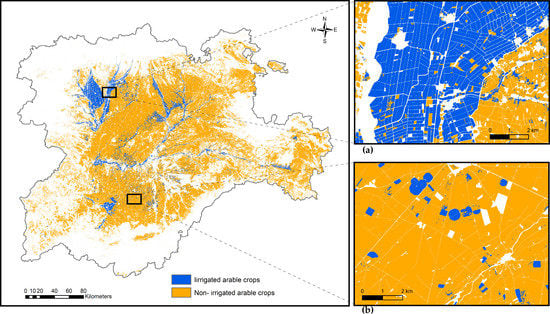
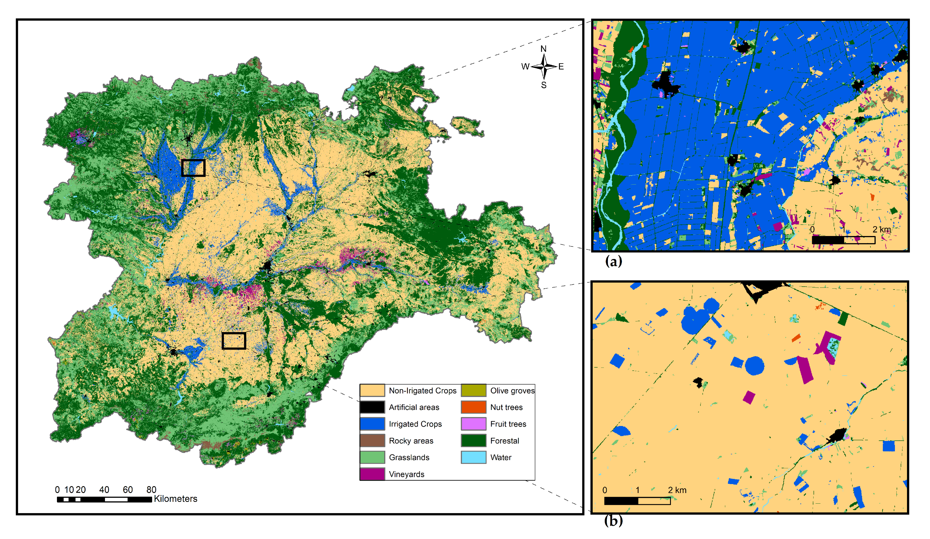
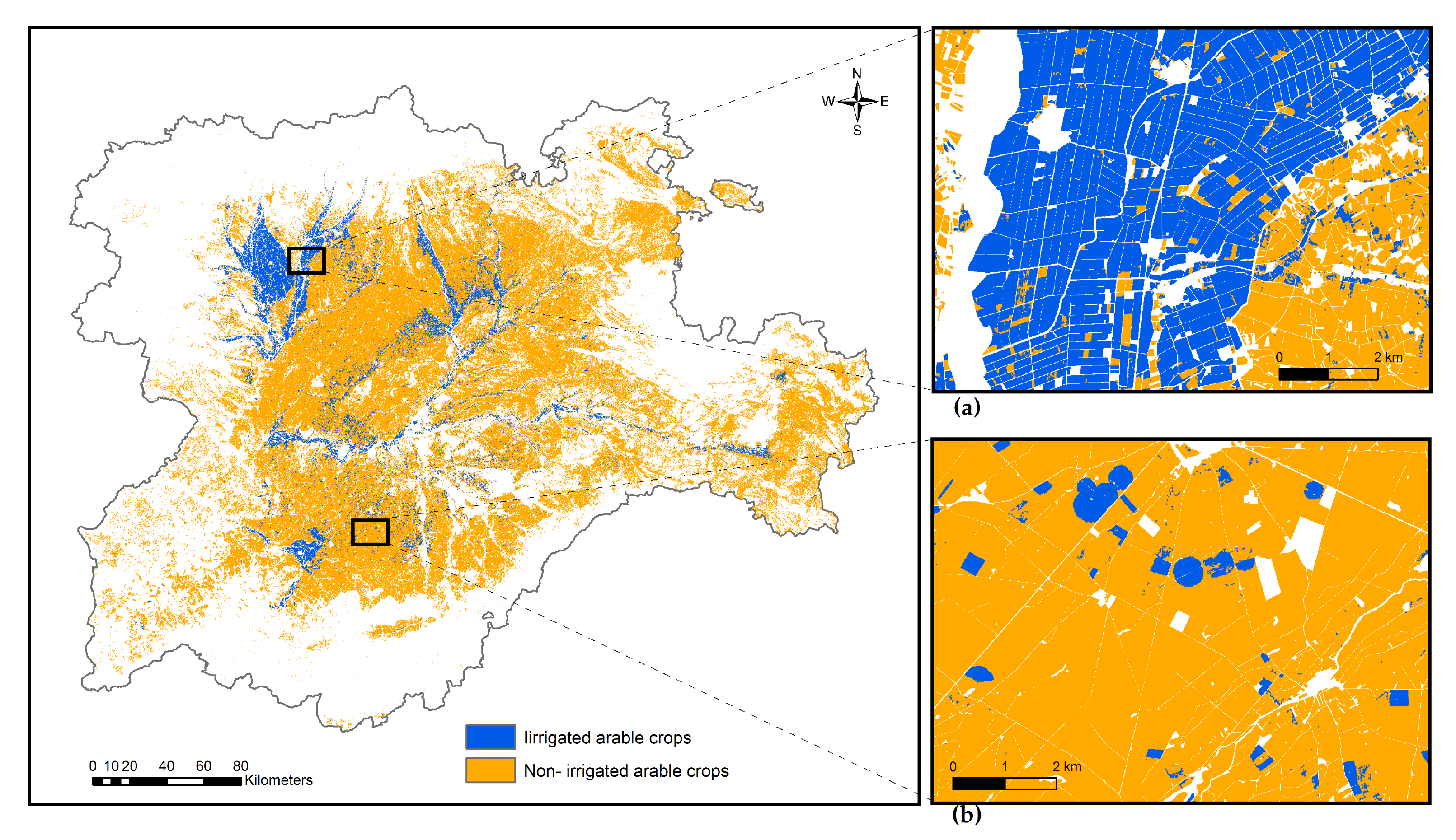
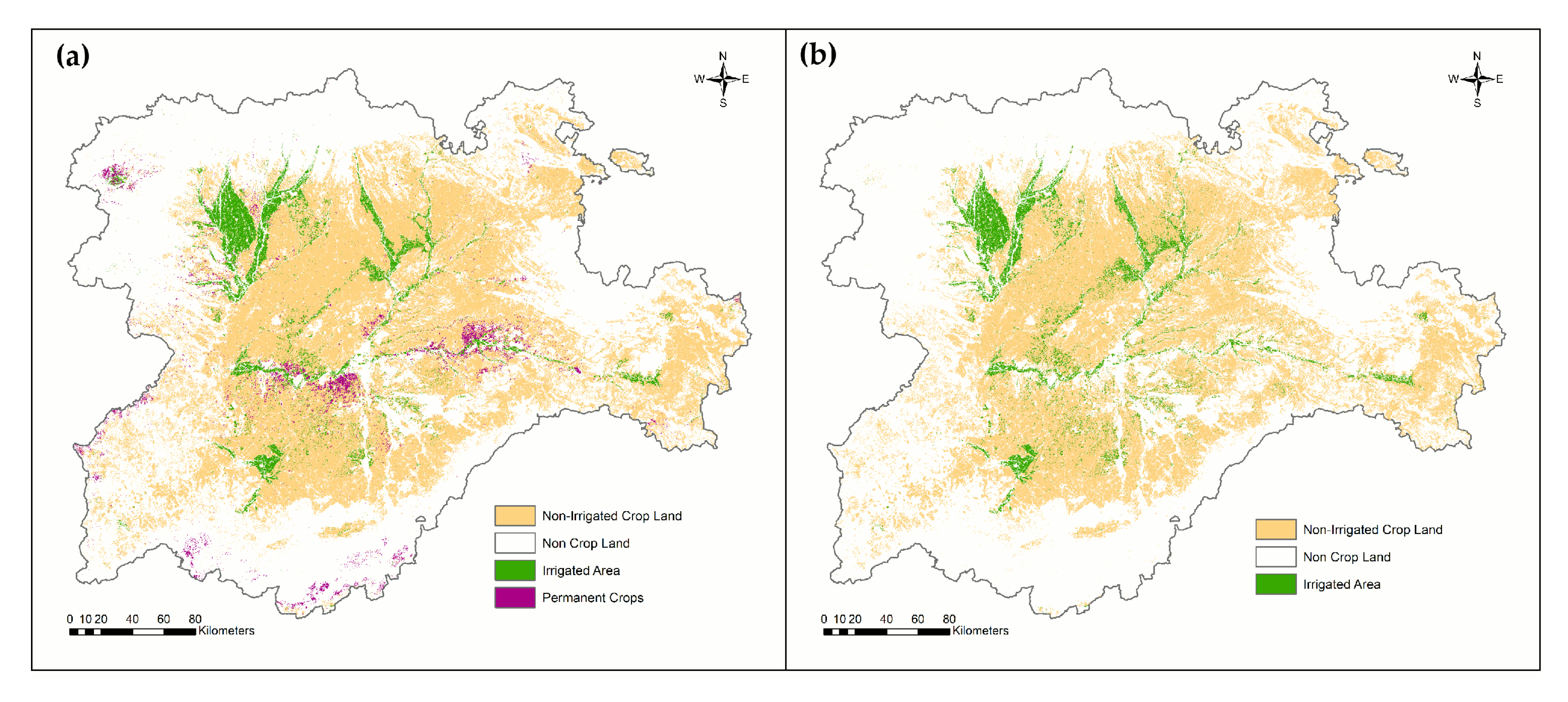
Both irrigation maps derived from the two procedures applied in this work have yielded similar results, not only regarding the accuracy measures but also in the allocations of the irrigated areas. Most of the irrigated plots detected are concentrated in the well-known irrigable areas in Castile and Leon (Figure 4 and Figure 5). Nevertheless, we can also detect, in both strategies, some rainfed fields within the irrigation areas, and on the contrary, we can detect sparse irrigation plots in the predominantly rainfed area (Figure 4 and Figure 5).

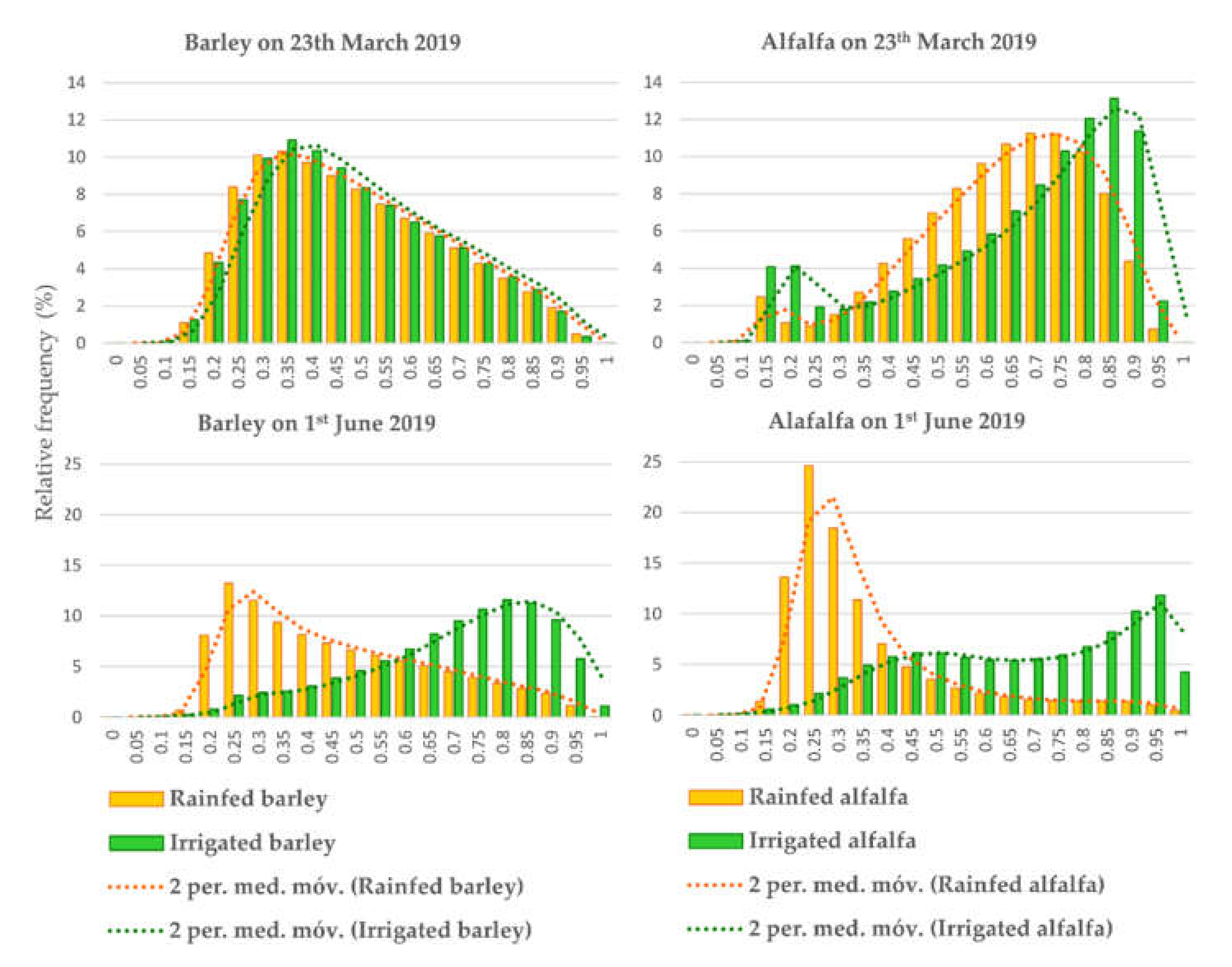
It is important to bear in mind that summer crops in irrigation agriculture are easier to identify due to the agroclimatic conditions existing in our region, given that crops such as corn, beet, and potato, among the most representative, are only cultivated in that season under irrigation. However, discriminating winter crops that can take place in both systems of cropping systems (irrigation and rainfed agriculture) is the real challenge, since the difference in spectral response between the two systems in spring is not as pronounced as in summer when water stress conditions cause rainfed crops to react to such stress [28]. For that reason, from the remote sensing approach, solving this situation is complicated. 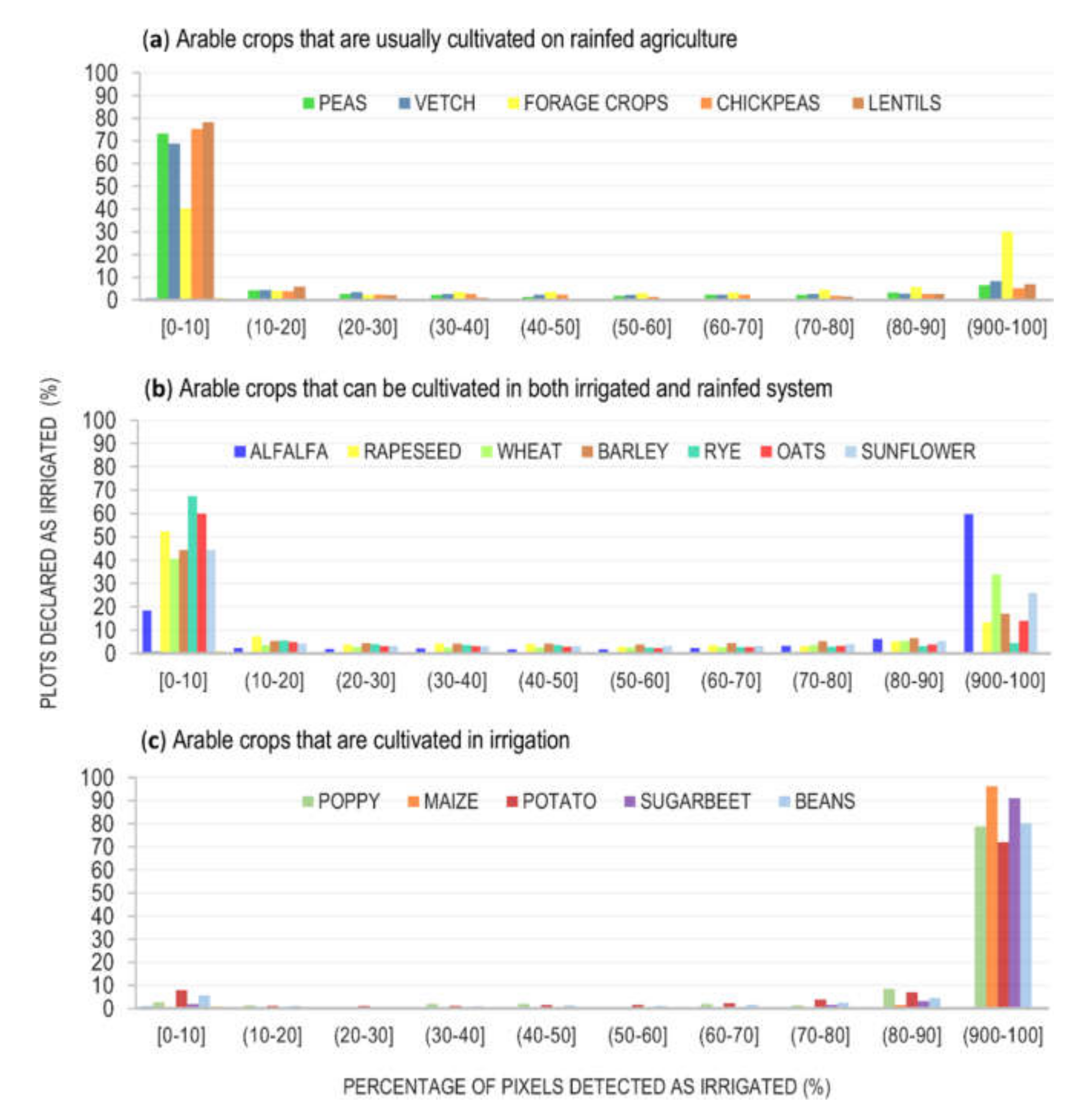However, the methodology proposed has been effective for this purpose, as it can be seen in Table A1, which shows the discrimination of the irrigation system in the most representative winter crops in the community of Castile and León, for instance, wheat which represents approximately 11% of the total area of the region (see Appendix A Table A2).

The discrimination between irrigated crops and rainfed crops that the methodology here presented offers, is of special relevance in the context of the CAP, since as we have already explained in the introduction, not only the crop identification is interesting but also the verification of compliance with some type of conditionality or cross-compliance. This is due to the fact that there are specific aids associated with certain crops that are only granted in a certain system, rainfed, or irrigated. Such is the case of aid associated with protein crops, specifically for alfalfa, which requires the crop not to be irrigated.

It should be noted that until now this technique has only been applied for the discrimination of certain herbaceous crops under irrigation. Meadows and woody crops (also permanent crops), among which the vineyard is the only significant one in Castile and León, have not been evaluated for several reasons that are explained. Firstly, the vineyard in this region is exclusively oriented to production under quality figures that impose restrictions on yield. Under these conditions, deficit irrigation is used to ensure the quality of the grapes, and therefore the differences between rainfed and irrigated are less. Furthermore, in vineyard cultivation, the soil/plant ratio is high, and therefore it is more difficult to detect changes in the hydric state of the crop by remote sensing.

Regarding the location and area estimation derived from both approaches, the results show similar figures. It is important to mention that we can also observe irrigation in minority crops in the IBM product. Figure 7 depicts the results of the total of irrigated and non-irrigated arable crops obtained from both strategies. In order to standardize results from both maps, some postprocessing steps have been carried out. A reclassification was done for the first approach map (HDTM) and the application of a mask of arable land extracted from the LPIS to both maps for representing only the herbaceous crops.

These large-area land cover maps also provide a clear added value for water allocation statistics in order to derive an estimation of the total irrigated agricultural area. It is important to keep in mind that the surface obtained by remote sensing refers to “effective” irrigation (actually watered surface), where satellite images objectively detect the pixels that behave as watered (Figure 4 and Figure 5). As has been reported previously [8,18], there is no unique and feasible source of information about this actual irrigated area. The comparison between the irrigated and non-irrigated arable cropland areas detected from both strategies, with similar area estimations (Figure 7 and Table 6), along with the fact that there is not a significant difference among the accuracy measures obtained from both maps show us that any of these maps might be a candidate to be implemented into the CAP monitoring system to detect if a declared field is actually irrigated. However, we can see an important advantage in using the IBM approach to support the aid control system, since the irrigation detection is not limited to the major crops previously defined in the reference dataset what occurs in the HDTM. Otherwise, any pixel can be identified as irrigated, regardless of the type of crop it belongs to. This allows us to identify irrigation even in minor crops, underrepresented on a regional scale, and therefore have not been included as data to train the classifier. This is also the explanation why the irrigated area estimation by the IBM is greater than that detected by the HDTM. Therefore, the map that has been chosen to be implemented into the regional aid control system has been the IBM.

Furthermore, thanks to the implementation methodology into the aid control system, there will be a marker related to irrigation in each claimed plot. Besides, it will inform about what percentage of pixels are identified as irrigated during the whole monitoring period within the agricultural parcel. The latter will allow us to have a more accurate estimation in the plots irrigated regularly. This is because we can detect not only if a plot is irrigated or not, but also if it has been irrigated on a regular basis and homogeneous way, or contrarily when an occasional irrigation event has been applied. The first case can be observed easily when most of the pixels inside the plot are detected as irrigated. However, when a low percentage of the pixels inside the plot has been detected as irrigated and there is an effect of “salt and pepper” within a plot, this usually indicates that there has been some occasional irrigation event to save the crop, for example when it suffers from water stress. Therefore, when a crop has been irrigated regularly is highly likely to be detected by this approach. On the other hand, when a crop has been watered occasionally, it might be that the change in its phenology may be unnoticed, and consequently also its detection. This will depend on several factors, the irrigation event date, the water consumption employed, and the timing when the irrigation has occurred. However, a further analysis was carried out to assess the difference between the number of parcels declared in the IACS as irrigated and the number identified as such in the IBM according to the percentage of pixels identified as irrigated within the agricultural parcel (Table 7). This could be very useful for agricultural statistics rather than to help CAP’s aid control system. To this end, an opposite analysis must be made. It must be seen if parcels declared in dryland farming have actually been watered. This is what really has an implication in the control of CAP’s aids, either because that plot did not have the right to use water for irrigation or because it is a specific requirement for some aids.

There is going to be an urgent need to implement a feasible methodology into any European CAP monitoring system to detect irrigation in the declared cropped fields to get some of the CAP subsidies. In the case of the Paying Agency of Castile and León the methodology here proposed as the second approach is going to be implemented this ongoing year 2020. Nevertheless, further research is required to improve accuracy results. We will certainly continue to pursue that aim, thus, for this year we are exploring the chances of introducing the Sentinel-1 images in the classification, and also, we are studying more vegetation indexes as the normalized difference moisture index (NDMI) or the normalized difference water index (NDWI) [4,16,17]. Another strategy we are going to research in the 2020 land cover classification is the stratification approach. Experimental results indicated that in large territories, a classification based on the stratification method achieved higher accuracies in the intensively cropped areas while the traditional method achieved higher accuracies in low or non-agricultural areas [29]. Therefore, we will make use of the agroclimatic zones raster prepared for the generation of the IBM, and we will use each zone as a stratum.

5. Conclusions

The results of this work are intended to support the CAP Integrated Administrative Control System in irrigation-related issues by means of intensive use of Sentinel-2 and decision tree supervised classification strategies. The proposed methodology allows us to perform a binary classification using information mainly contained in the IACS itself without specific fieldwork with very high accuracy (0.92 kappa index). The derivation of an irrigation binary maps is meant to be a relevant source of information for the CAP decision-making system and the eligibility of the farmers’ application. Besides, the methodology to implement that information into the CAP control system makes it suitable to be operational into the aids control system as suggested by the European Court of Auditors.

References

1. European Union. DG AGRI. Commission Implementing Regulation (EU) 2018/746 of 18 May 2018 amending Implementing Regulation (EU) No 809/2014 as regards modification of single applications and payment claims and checks. Off. J. Eur. Union 2018, 125, 1–7. Available online: http://data.europa.eu/eli/reg_impl/2018/746/oj (accessed on 10 April 2020).
2. Castile and León Crops and Natural Land Map (MCSNCyL). Available online: http://mcsncyl.itacyl.es/en/inicio (accessed on 10 April 2020).
3. Pareeth, S.; Karimi, P.; Shafiei, M.; De Fraiture, C. Mapping agricultural landuse patterns from time series of Landsat 8 using random forest based hierarchial approach. Remote Sens. 2019, 11, 601. [Google Scholar] [CrossRef] [Green Version]
4. Kyere, I.; Astor, T.; Graß, R.; Wachendorf, M. Multi-Temporal Agricultural Land-Cover Mapping Using Single-Year and Multi-Year Models Based on Landsat Imagery and IACS Data. Agronomy 2019, 9, 309. [Google Scholar] [CrossRef] [Green Version]
5. ESA-CCI Land Cover Product. Available online: http://maps.elie.ucl.ac.be/CCI/viewer/index.php (accessed on 10 April 2020).
6. Siebert, S.; Henrich, V.; Frenken, K.; Burke, J. Global Map of Irrigation Areas Version 5; Germany/Food and Agriculture Organization of the United Nations; Rheinische Friedrich-Wilhelms-University: Rome, Italy, 2013; Available online: http://www.fao.org/aquastat/en/geospatial-information/global-maps-irrigated-areas/latest-version (accessed on 10 April 2020).
7. Thenkabail, P.S.; Biradar, C.M.; Turral, H.; Noojipady, P.; Li, Y.J.; Dheeravath, V.; Cai, X.L.; Velpuri, M.; Vithanage, J.; Schull, M.; et al. A Global Irrigated Area Map (GIAM) using time-series satellite sensor, secondary, Google Earth, and Groundtruth data. Int. J. Remote Sens. 2009, 30, 3679–3733. Available online: https://waterdata.iwmi.org/Applications/GIAM2000/ (accessed on 10 April 2020). [CrossRef]
8. Gómez, V.P.; Medina, V.D.B.; Bengoa, J.L.; García, D.A.N. Accuracy assessment of a 122 classes land cover map based on Sentinel-2, Landsat 8 and Deimos-1 images and ancillary data. In Proceedings of the 2018 IEEE International Geoscience and Remote Sensing Symposium (IGARSS), Valencia, Spain, 22–27 July 2018; pp. 5453–5456. [Google Scholar]
9. Bea Martínez, M.; Rodríguez Esteban, J.A.; Montesinos Aranda, S. Uso de técnicas de información geográfica para la discriminación de superficies regadas. Rev. Int. Cienc. Tecnol. Inf. Geográfica 2013, 13, 220–245. [Google Scholar]
10. Ozdogan, M.; Gutman, G. A new methodology to map irrigated areas using multi-temporal MODIS and ancillary data: An application example in the continental US. Remote Sens. Environ. 2008, 112, 3520–3537. [Google Scholar] [CrossRef] [Green Version]
11. Ambika, A.K.; Wardlow, B.; Mishra, V. Remotely sensed high resolution irrigated area mapping in India for 2000 to 2015. Sci. Data 2016, 3, 160118. [Google Scholar] [CrossRef] [PubMed] [Green Version]
12. Conrad, C.; Fritsch, S.; Zeidler, J.; Rücker, G.; Dech, S. Per-field irrigated crop classification in arid Central Asia using SPOT and ASTER data. Remote Sens. 2010, 2, 1035–1056. [Google Scholar] [CrossRef] [Green Version]
13. Vogels, M.F.; De Jong, S.M.; Sterk, G.; Addink, E.A. Mapping irrigated agriculture in complex landscapes using SPOT6 imagery and object-based image analysis–A case study in the Central Rift Valley, Ethiopia. Int. J. Appl. Earth Obs. Geoinf. 2019, 75, 118–129. [Google Scholar] [CrossRef]
14. Xiang, K.; Ma, M.; Liu, W.; Dong, J.; Zhu, X.; Yuan, W. Mapping Irrigated Areas of Northeast China in Comparison to Natural Vegetation. Remote Sens. 2019, 11, 825. [Google Scholar] [CrossRef] [Green Version]
15. Ferrant, S.; Selles, A.; Le Page, M.; Herrault, P.A.; Pelletier, C.; Al-Bitar, A.; Mermoz, S.; Gascoin, S.; Bouvet, A.; Saqalli, M.; et al. Detection of irrigated crops from Sentinel-1 and Sentinel-2 data to estimate seasonal groundwater use in South India. Remote Sens. 2017, 9, 1119. [Google Scholar] [CrossRef] [Green Version]
16. Bazzi, H.; Baghdadi, N.; Ienco, D.; El Hajj, M.; Zribi, M.; Belhouchette, H.; Escorihuela, M.J.; Demarez, V. Mapping Irrigated Areas Using Sentinel-1 Time Series in Catalonia, Spain. Remote Sens. 2019, 11, 1836. [Google Scholar] [CrossRef] [Green Version]
17. Demarez, V.; Helen, F.; Marais-Sicre, C.; Baup, F. In-season mapping of irrigated crops using Landsat 8 and Sentinel-1 time series. Remote Sens. 2019, 11, 118. [Google Scholar] [CrossRef] [Green Version]
18. Paredes-Gómez, V.; Del Blanco-Medina, V.; Gutiérrez-García, A.; Nafría-García, D.A. Seguimiento y evaluación de la capacidad de discriminación de cultivos herbáceos en regadío a partir de imágenes de satélite en el periodo 2016-2018, In Teledetección: Hacia una visión global del cambio climático. In Proceedings of the XVIII Congress of the Spanish Association of Remote Sensing, Valladolid, Spain, 24–27 September 2019; pp. 15–18. [Google Scholar]
19. Boryan, C.; Yang, Z.; Mueller, R.; Craig, M. Monitoring US agriculture: The US Department of Agriculture, National Agricultural Statistics Service, Cropland Data Layer Program. Geocarto Int. 2011, 26, 341–358. [Google Scholar] [CrossRef]
20. Pal, M.; Mather, P.M. An assessment of the effectiveness of decision tree methods for land cover classification. Remote Sens. Environ. 2003, 86, 554–565. [Google Scholar] [CrossRef]
21. Inglada, J.; Arias, M.; Tardy, B.; Hagolle, O.; Valero, S.; Morin, D.; Dedieu, G.; Sepulcre, G.; Bontemps, S.; Defourny, P.; et al. Assessment of an operational system for crop type map production using high temporal and spatial resolution satellite optical imagery. Remote Sens. 2015, 7, 12356–12379. [Google Scholar] [CrossRef] [Green Version]
22. Quinlan, J.R. C4.5: Programs for Machine Learning; Morgan Kaufmann Publishers Inc.: San Francisco, CA, USA, 1993. [Google Scholar]
23. Oukrop, C.M.; Evans, D.M.; Bartos, D.L.; Ramsey, R.D.; Ryel, R.J. Moderate-Scale Mapping Methods of Aspen Stand Types: A Case Study for Cedar Mountain in Southern Utah; Gen. Tech. Rep. RMRS-GTR-259; US Department of Agriculture, Forest Service, Rocky Mountain Research Station: Fort Collins, CO, USA, 2011.
24. GRASS GISS (Geographic Resources Analysis Support System) Module R.Kappa. Available online: https://grass.osgeo.org/grass74/manuals/r.kappa.html (accessed on 10 April 2020).
25. Cochran, W.G. Sampling Techniques, 3rd ed.; John Wiley & Sons: Hoboken, NJ, USA, 1977. [Google Scholar]
26. Chicco, D.; Jurman, G. The advantages of the Matthews correlation coefficient (MCC) over F1 score and accuracy in binary classification evaluation. BMC Genom. 2020, 21, 6. [Google Scholar] [CrossRef] [PubMed] [Green Version]
27. Griffiths, P.; Nendel, C.; Hostert, P. Intra-annual reflectance composites from Sentinel-2 and Landsat for national-scale crop and land cover mapping. Remote Sens. Environ. 2019, 220, 135–151. [Google Scholar] [CrossRef]
28. Reddy, A.R.; Chaitanya, K.V.; Vivekanandan, M. Drought-induced responses of photosynthesis and antioxidant metabolism in higher plants. J. Plant Physiol. 2004, 161, 1189–1202. [Google Scholar] [CrossRef] [PubMed]
29. Boryan, C.G.; Yang, Z. A new land cover classification based stratification method for area sampling frame construction. In Proceedings of the 2012 First International Conference on Agro-Geoinformatics, Shanghai, China, 2–4 August 2012; pp. 1–6. [Google Scholar]
Figure 1. (a) Geographical location of the region of Castile and Leon in Europe; (b) Digital Elevation Model (DEM) of the study area. Coordinate system: ETRS89 UTM Zone 30 N.
Agronomy 10 00867 g001
Figure 2. (a) All Sentinel-2 granules covering Castile and León (94,224 km2). (b) Sentinel-2 orbits over the study area: R037, R137, and R094.
Agronomy 10 00867 g002
Figure 3. Histogram of NDVI (Normalized Difference Vegetation Index) values of irrigated (in green) and non-irrigated (in yellow) crops. The two right-hand figures showing Alfalfa values, and on the left hand are the figures depicting barley values. There are two different dates illustrated: 23rd March (upper plots) and 1st June (lower plot).
Agronomy 10 00867 g003
Figure 4. Crop and natural land classification map over the study area of Castile and León for 2019 obtained with the Highly Detailed Thematic Map (HDTM). A reduction in the legend classes has been applied for better visualization of the main land cover classes grouped. (a) Detail of a large irrigated area dedicated mainly to maize in León province. (b) Detail of a predominately rainfed area dominated by winter cereals, such as barley, but where some irrigated field can be detected (in blue).
Agronomy 10 00867 g004
Figure 5. Irrigation Binary Map (IBM) over the study area of Castile and León for 2019 obtained with the binary classification strategy to detect irrigation. (a) Detail of a large irrigated area dedicated mainly to maize in León province. (b) Detail of a predominately rainfed area dominated by winter cereals, such as barley, but where some irrigated fields can be detected (in blue). To achieve a better understanding of the extent of arable crops in the region, a mask obtained from the Land Parcel Information System (LPIS) layer containing only the land use defined as arable land, has been applied to this map.
Agronomy 10 00867 g005
Figure 6. Distribution of parcels declared as irrigated in the Integrated Administrative Control System (IACS) according to the percentage of pixels detected as irrigated in the Irrigation binary map (IBM). The x axis represents the percentage of the pixels irrigated within each plot grouped in 10% steps, and the Y axis depicts the percentage of plots declared as irrigated that falls into each group. (a) Arable crops that are usually cultivated on rainfed agriculture; (b) Arable crops that can be cultivated in both irrigated and rainfed system; (c) Arable crops that are normally irrigated crops.
Agronomy 10 00867 g006
Figure 7. Comparison between the results of the total of irrigated and non-irrigated arable crops obtained from both strategies: (a) irrigated, non-irrigated, permanent crops, and non-crop areas detected using the High detailed thematic map (HDTM). Note that permanent crops, mainly vineyard in our region, have been separated into a separate class to differentiate them from rainfed crops. (b) irrigated, non-irrigated, and non-crop areas detected employing the Irrigation binary map (IBM).
Agronomy 10 00867 g007