A Comparison of Moment-Independent and Variance-Based Global Sensitivity Analysis Approaches for Wheat Yield Estimation with the Aquacrop-OS Model

 ,
,  ,
,  ,
,  ,
, 

Abstract
1. Introduction
2. Materials and Methods
2.1. Sensitivity Analysis
2.1.1. Morris-Based Elementary Effects
2.1.2. EFAST Method
2.1.3. Density-Based PAWN Method
2.1.4. Identifying Non-Influential Parameters by Using a Dummy Parameter
2.2. Crop Model: Aquacrop Open Source
2.3. Setting up the Parameters for AOS Model
2.4. Sites Description
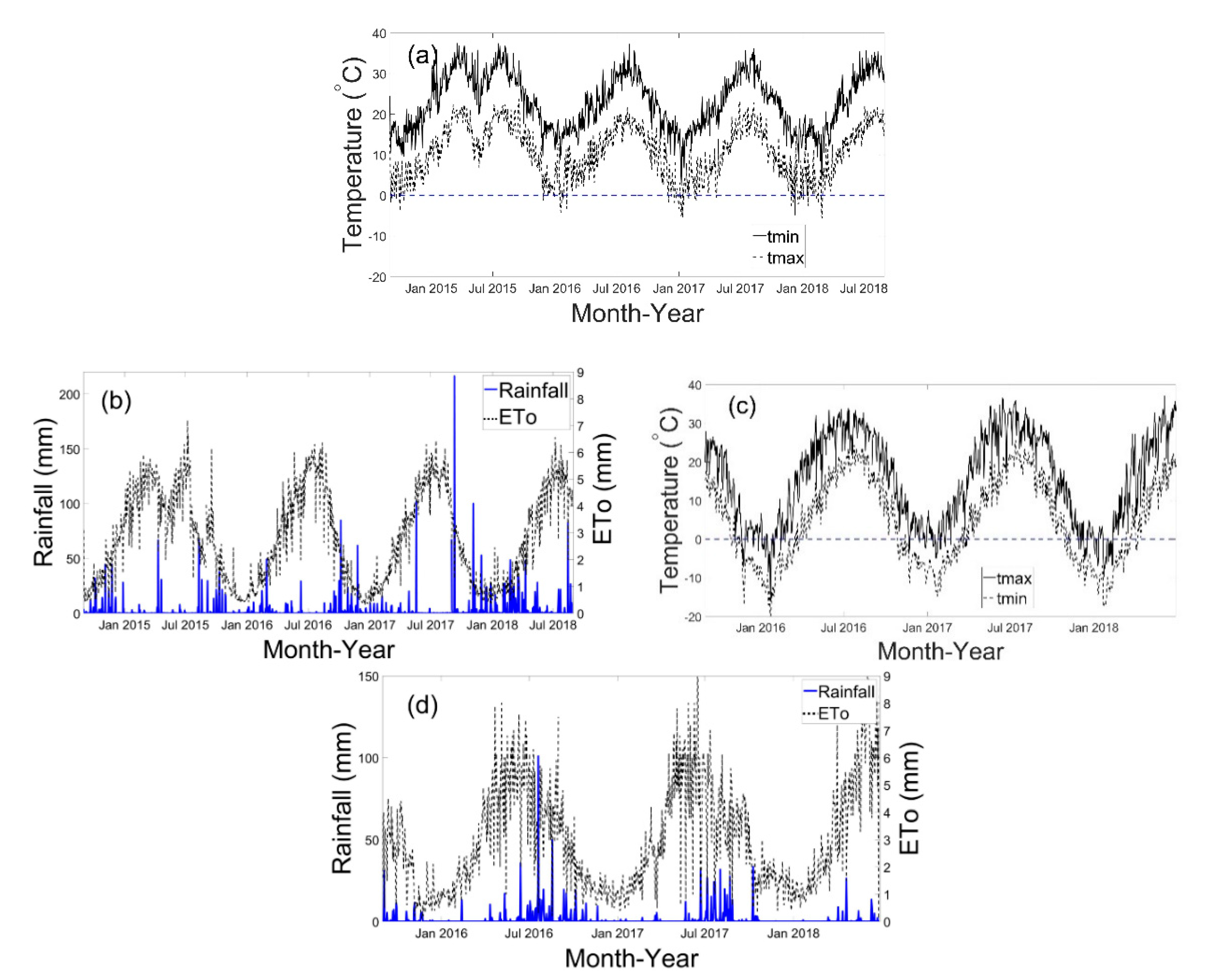
2.5. Weather Data
3. Results
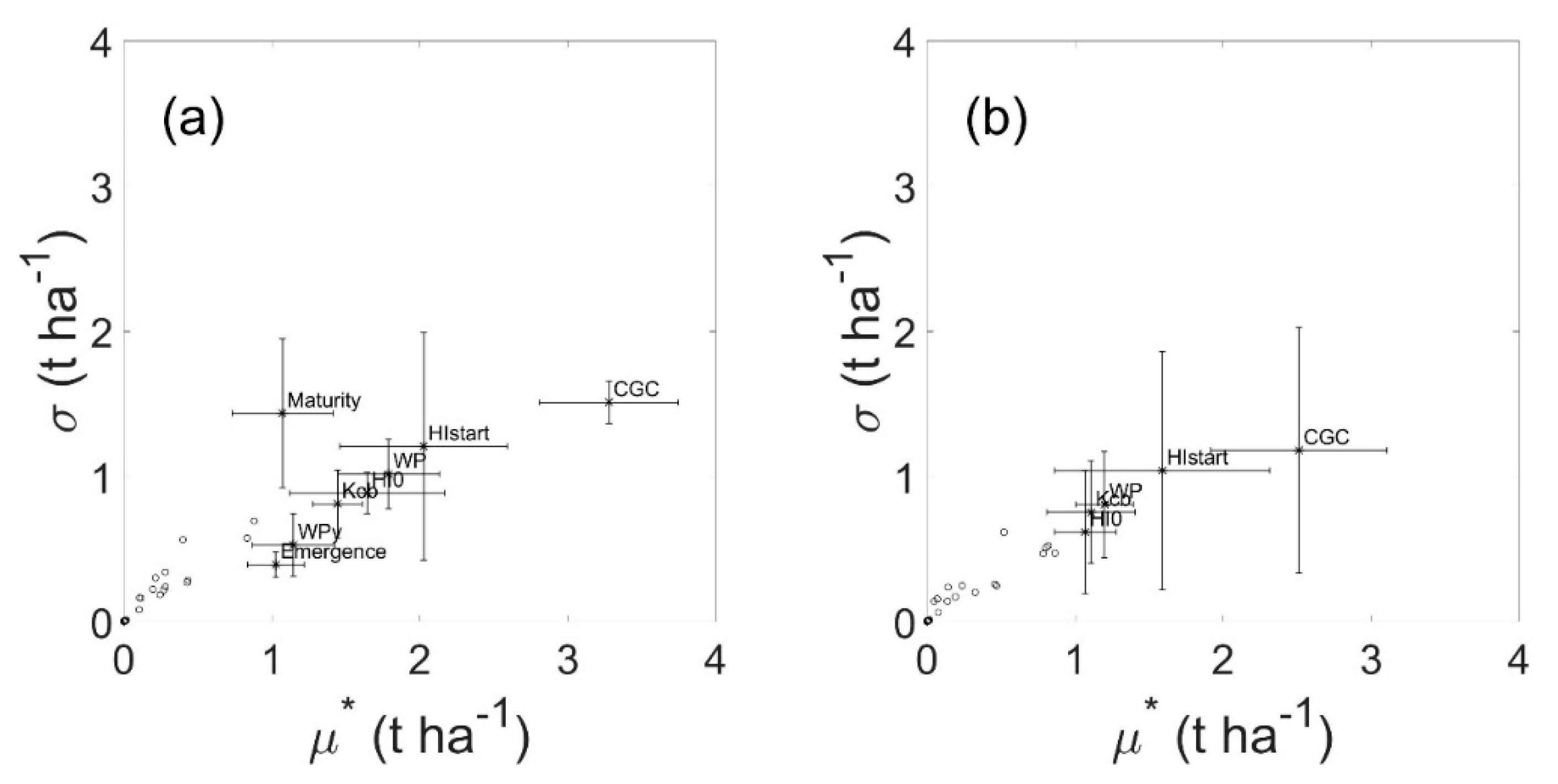
3.1. Morris Method
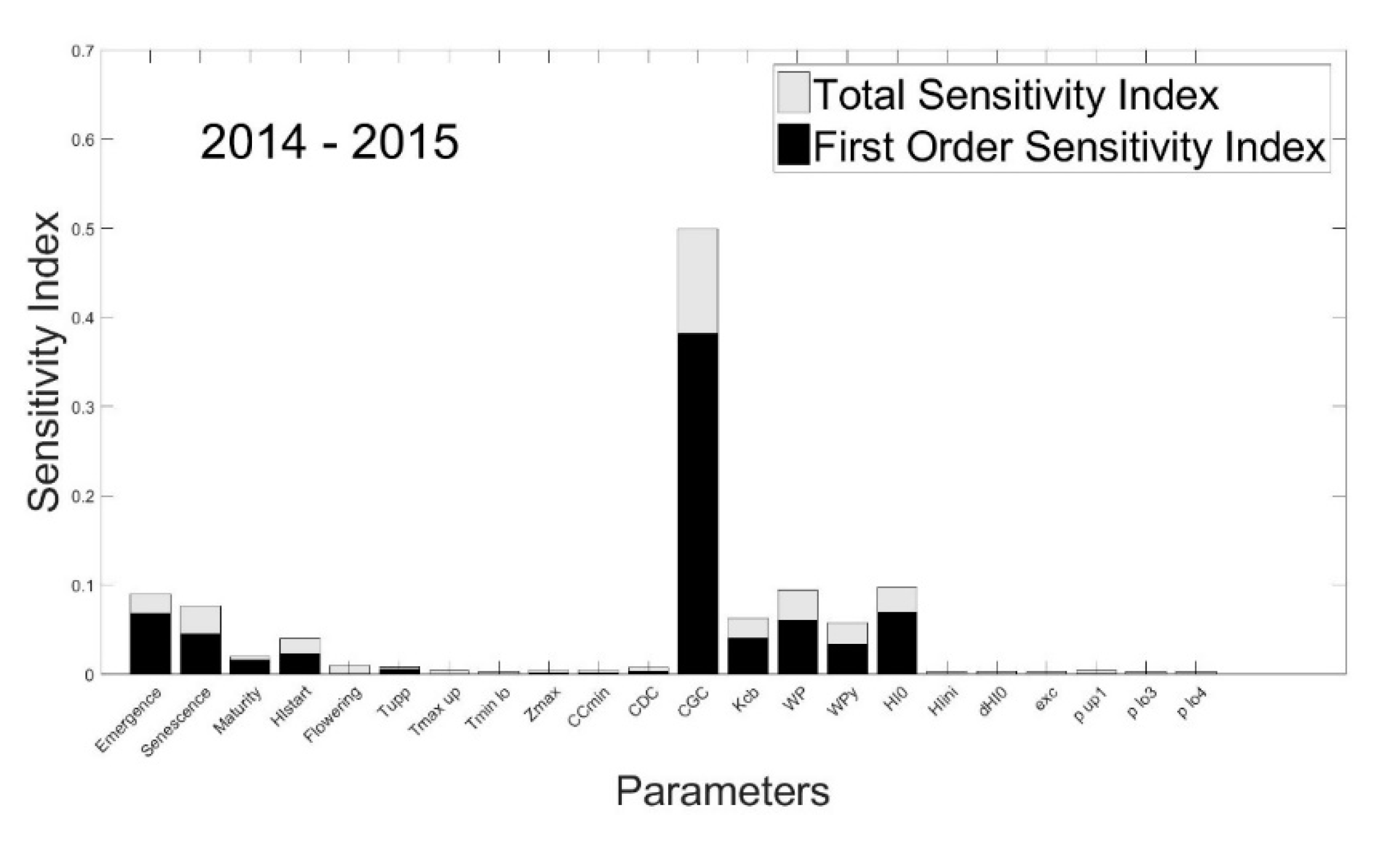
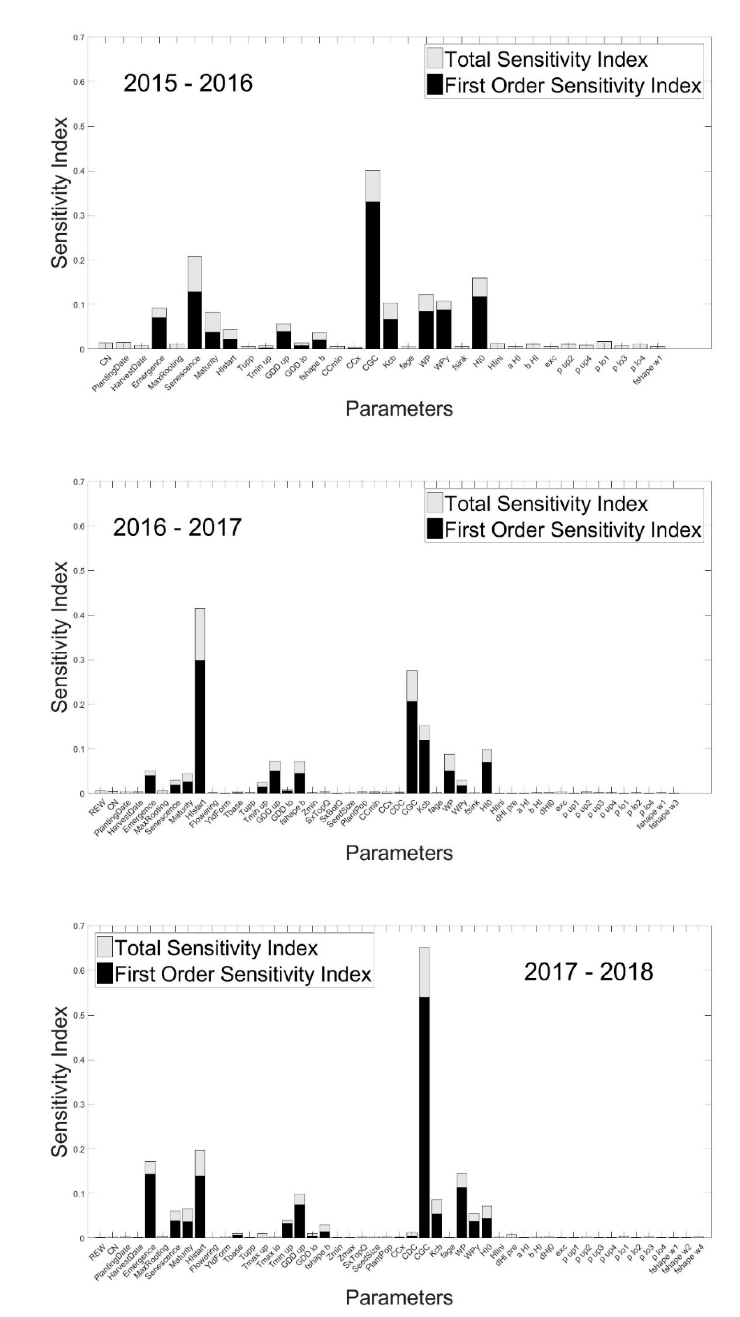
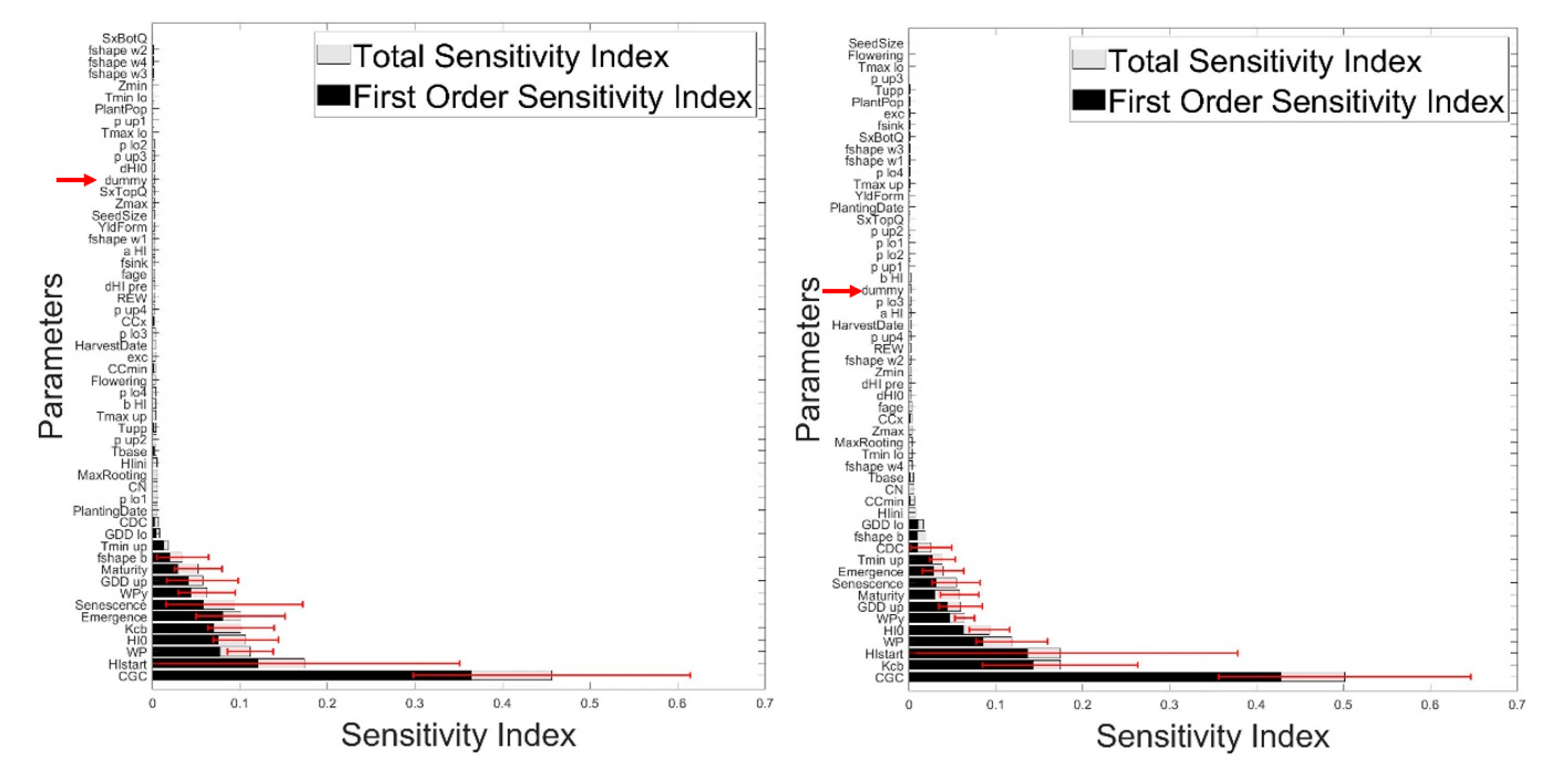
3.2. Variance-Based Extended Fourier Amplitude Sensitivity Test (EFAST)
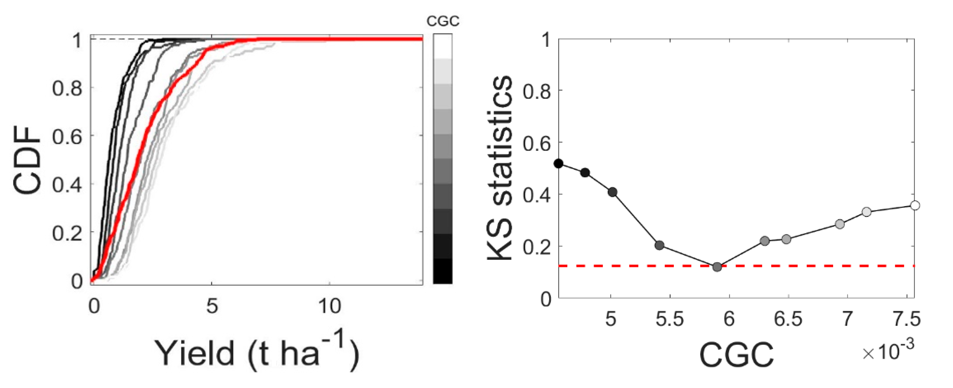
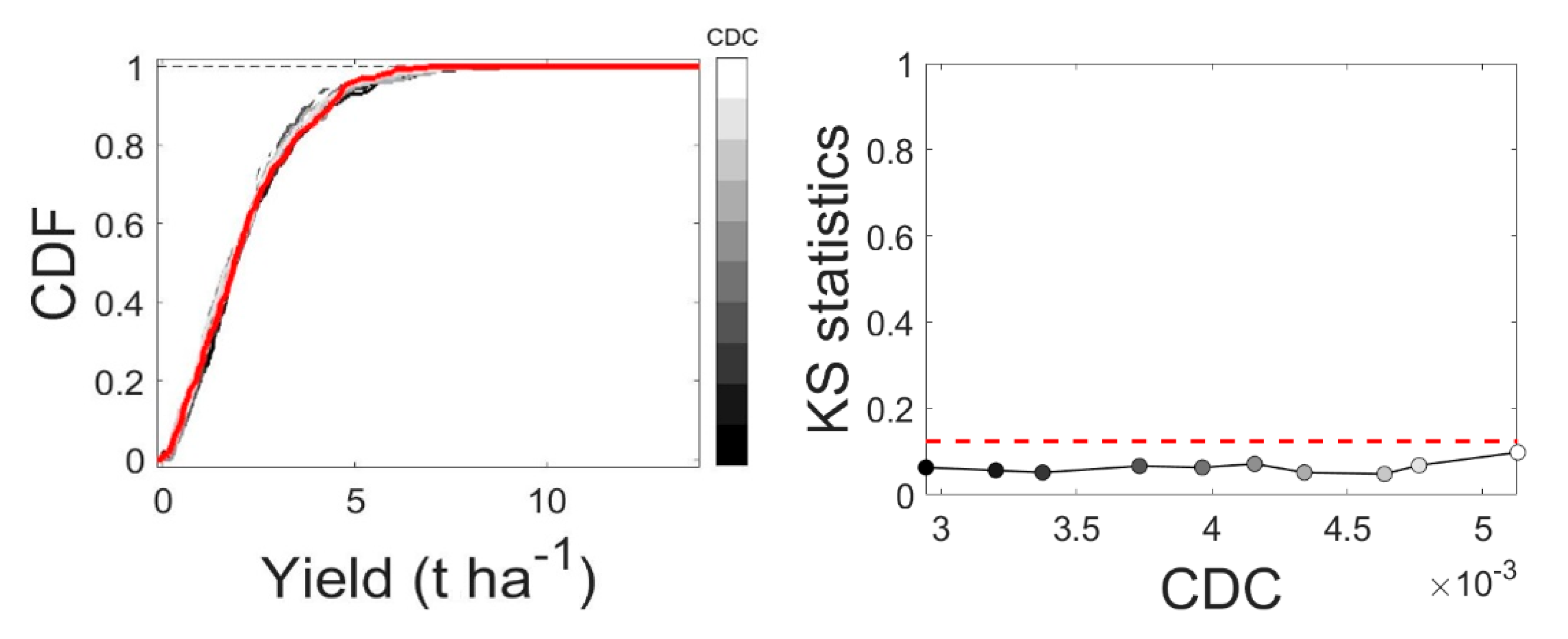
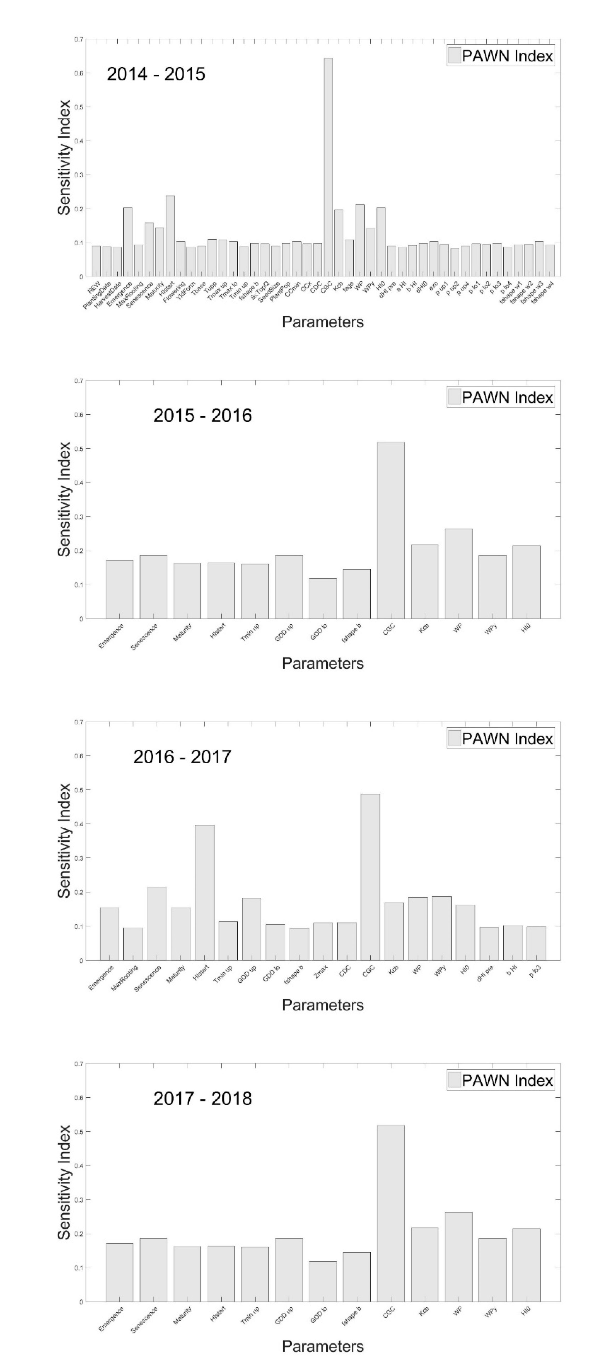
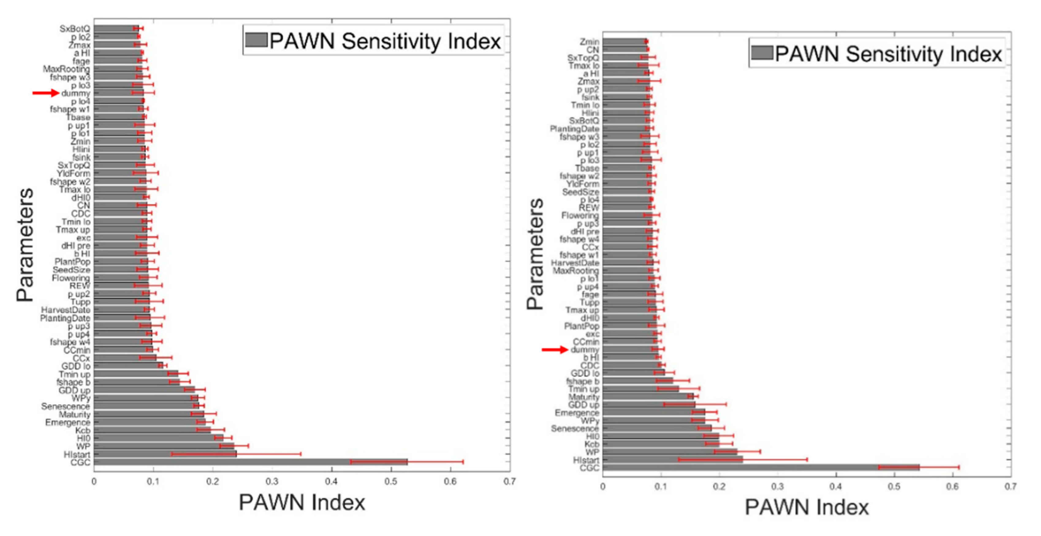
3.3. Density-Based PAWN Method
4. Discussion
4.1. Elementary Effects Using the Morris Method
4.2. Variance-Based Extended Fourier Amplitude Sensitivity Test (EFAST)
4.3. Density-Based PAWN Method
4.4. Sensitive Parameters in Relation to Model Processes and Agronomic Conditions
5. Conclusions
Supplementary Materials
Author Contributions
Funding
Acknowledgments
Conflicts of Interest
References
- De Willigen, P. Nitrogen turnover in the soil-crop system; comparison of fourteen simulation models. In Nitrogen Turnover in the Soil-Crop System; Springer: Dordrecht, The Netherlands, 1991; pp. 141–149. [Google Scholar]
- Hopmans, J.W.; Bristow, K.L. Current capabilities and future needs of root water and nutrient uptake modeling. Adv. Agr. 2002, 77, 104–175. [Google Scholar]
- Gervois, S.; de Noblet-Ducoudré, N.; Viovy, N.; Ciais, P.; Brisson, N.; Seguin, B.; Perrier, A. Including croplands in a global biosphere model: Methodology and evaluation at specific sites. Earth Interact. 2004, 8, 1–25. [Google Scholar] [CrossRef]
- Saltelli, A.; Tarantola, S.; Campolongo, F. Sensitivity anaysis as an ingredient of modeling. Stat. Sci. 2000, 15, 377–395. [Google Scholar]
- Wallach, D.; Goffinet, B.; Bergez, J.-E.; Debaeke, P.; Leenhardt, D.; Aubertot, J.-N. Parameter estimation for crop models. Agron. J. 2001, 93, 757–766. [Google Scholar] [CrossRef]
- Makowski, D.; Hillier, J.; Wallach, D.; Andrieu, B.; Jeuffroy, M. Parameter Estimation for Crop Models. Working with Dynamic Crop Models; Wallach, D., Makowski, D., Jones, J., Eds.; Elsevier: Amsterdam, The Netherlands, 2006; pp. 101–149. [Google Scholar]
- Silvestro, P.C.; Pignatti, S.; Yang, H.; Yang, G.; Pascucci, S.; Castaldi, F.; Casa, R. Sensitivity analysis of the Aquacrop and SAFYE crop models for the assessment of water limited winter wheat yield in regional scale applications. PLoS ONE 2017, 12, e0187485. [Google Scholar] [CrossRef] [PubMed]
- Yapo, P.O.; Gupta, H.V.; Sorooshian, S. Multi-objective global optimization for hydrologic models. J. Hydrol. 1998, 204, 83–97. [Google Scholar] [CrossRef]
- Vrugt, J.A.; Bouten, W.; Gupta, H.V.; Sorooshian, S. Toward improved identifiability of hydrologic model parameters: The information content of experimental data. Water Resour. Res. 2002, 38, 48–61. [Google Scholar] [CrossRef]
- Vrugt, J.A.; Gupta, H.V.; Bouten, W.; Sorooshian, S. A Shuffled Complex Evolution Metropolis algorithm for optimization and uncertainty assessment of hydrologic model parameters. Water Resour. Res. 2003, 39, 1–14. [Google Scholar] [CrossRef]
- Pianosi, F.; Beven, K.; Freer, J.; Hall, J.W.; Rougier, J.; Stephenson, D.B.; Wagener, T. Sensitivity analysis of environmental models: A systematic review with practical workflow. Environ. Model. Softw. 2016, 79, 214–232. [Google Scholar] [CrossRef]
- Duan, Q.; Sorooshian, S.; Gupta, V. Effective and efficient global optimization for conceptual rainfall-runoff models. Water Resour. Res. 1992, 28, 1015–1031. [Google Scholar] [CrossRef]
- Bekele, E.G.; Nicklow, J.W. Multi-objective automatic calibration of SWAT using NSGA-II. J. Hydrol. 2007, 341, 165–176. [Google Scholar] [CrossRef]
- Nossent, J.; Elsen, P.; Bauwens, W. Sobol’ sensitivity analysis of a complex environmental model. Environ. Model. Softw. 2011, 26, 1515–1525. [Google Scholar] [CrossRef]
- Wallach, D.; Makowski, D.; Jones, J.W.; Brun, F.; Jones, J.W. Working with Dynamic Crop Models; Academic Press: Cambridge, MA, USA, 2014; pp. 407–436. [Google Scholar]
- Saltelli, A.; Ratto, M.; Andres, T.; Campolongo, F.; Cariboni, J.; Gatelli, D. Global Sensitivity Analysis: The Primer; John Wiley & Sons: West Sussex, UK, 2008. [Google Scholar]
- Iooss, B.; Lemaître, P. A review on global sensitivity analysis methods. In Uncertainty Management in Simulation-Optimization of Complex Systems; Springer: Boston, MA, USA, 2015; pp. 101–122. [Google Scholar]
- Chen, Y.; Cournède, P.-H. Data assimilation to reduce uncertainty of crop model prediction with convolution particle filtering. Ecol. Model. 2014, 290, 165–177. [Google Scholar] [CrossRef]
- Saltelli, A.; Tarantola, S.; Chan, K.-S. A quantitative model-independent method for global sensitivity analysis of model output. Technometrics 1999, 41, 39–56. [Google Scholar] [CrossRef]
- Cariboni, J.; Gatelli, D.; Liska, R.; Saltelli, A. The role of sensitivity analysis in ecological modelling. Ecol. Model. 2007, 203, 167–182. [Google Scholar] [CrossRef]
- Sobol’, I.M. On sensitivity estimation for nonlinear mathematical models. Matem. Mod. 1990, 2, 112–118. [Google Scholar]
- Saltelli, A.; Chan, K.; Scott, M. Sensitivity Analysis: Probability and Statistics Series; John and Wiley & Sons: New York, NY, USA, 2000; pp. 3–14. [Google Scholar]
- Van Griensven, A.V.; Meixner, T.; Grunwald, S.; Bishop, T.; Diluzio, M.; Srinivasan, R. A global sensitivity analysis tool for the parameters of multi-variable catchment models. J. Hydrol. 2006, 324, 10–23. [Google Scholar] [CrossRef]
- Borgonovo, E. A new uncertainty importance measure. Reliab. Eng. Syst. Saf. 2007, 92, 771–784. [Google Scholar] [CrossRef]
- Pianosi, F.; Wagener, T. A simple and efficient method for global sensitivity analysis based on cumulative distribution functions. Environ. Model. Softw. 2015, 67, 1–11. [Google Scholar] [CrossRef]
- Saltelli, A. Sensitivity analysis for importance assessment. Risk Analysis 2002, 22, 579–590. [Google Scholar] [CrossRef]
- Liu, H.; Chen, W.; Sudjianto, A. Relative entropy based method for probabilistic sensitivity analysis in engineering design. J. Mech. Des. 2006, 128, 326–336. [Google Scholar] [CrossRef]
- Borgonovo, E.; Castaings, W.; Tarantola, S. Moment independent importance measures: New results and analytical test cases. Risk Analysis: An International Journal 2011, 31, 404–428. [Google Scholar] [CrossRef] [PubMed]
- Zadeh, F.K.; Nossent, J.; Sarrazin, F.; Pianosi, F.; van Griensven, A.; Wagener, T.; Bauwens, W. Comparison of variance-based and moment-independent global sensitivity analysis approaches by application to the SWAT model. Environ. Model. Softw. 2017, 91, 210–222. [Google Scholar] [CrossRef]
- Steduto, P.; Hsiao, T.C.; Raes, D.; Fereres, E. AquaCrop—The FAO crop model to simulate yield response to water: I. Concepts and underlying principles. Agron J. 2009, 101, 426–437. [Google Scholar] [CrossRef]
- Foster, T.; Brozović, N.; Butler, A.P.; Neale, C.M.U.; Raes, D.; Steduto, P.; Fereres, E.; Hsiao, T.C. AquaCrop-OS: An open source version of FAO’s crop water productivity model. Agric. Water Manag. 2017, 181, 18–22. [Google Scholar] [CrossRef]
- Todorovic, M.; Albrizio, R.; Zivotic, L.; Saab, M.-T.A.; Stöckle, C.; Steduto, P. Assessment of AquaCrop, CropSyst, and WOFOST models in the simulation of sunflower growth under different water regimes. Agron J. 2009, 101, 509–521. [Google Scholar] [CrossRef]
- Saab, M.T.A.; Todorovic, M.; Albrizio, R. Comparing AquaCrop and CropSyst models in simulating barley growth and yield under different water and nitrogen regimes. Does calibration year influence the performance of crop growth models? Agric. Water Manag. 2015, 147, 21–33. [Google Scholar] [CrossRef]
- Xiangxiang, W.; Quanjiu, W.; Jun, F.; Qiuping, F. Evaluation of the AquaCrop model for simulating the impact of water deficits and different irrigation regimes on the biomass and yield of winter wheat grown on China’s Loess Plateau. Agric. Water Manag. 2013, 129, 95–104. [Google Scholar] [CrossRef]
- Jin, X.; Feng, H.; Zhu, X.; Li, Z.; Song, S.; Song, X.; Yang, G.; Xu, X.; Guo, W. Assessment of the AquaCrop model for use in simulation of irrigated winter wheat canopy cover, biomass, and grain yield in the North China Plain. PLoS ONE 2014, 9, e86938. [Google Scholar] [CrossRef]
- Foster, T. AquaCrop-OS v6.0a Reference Manual; FAO: Rome, Italy, 2019. [Google Scholar]
- Vanuytrecht, E.; Raes, D.; Willems, P. Global sensitivity analysis of yield output from the water productivity model. Environ. Model. Softw. 2014, 51, 323–332. [Google Scholar] [CrossRef]
- Xing, H.; Xu, X.; Li, Z.; Chen, Y.; Feng, H.; Yang, G.; Chen, Z. Global sensitivity analysis of the AquaCrop model for winter wheat under different water treatments based on the extended Fourier amplitude sensitivity test. J. Integr. Agric. 2017, 16, 2444–2458. [Google Scholar] [CrossRef]
- Morris, M.D. Factorial sampling plans for preliminary computational experiments. Technometrics 1991, 33, 161–174. [Google Scholar] [CrossRef]
- Campolongo, F.; Cariboni, J.; Saltelli, A. An effective screening design for sensitivity analysis of large models. Environ. Model. Softw. 2007, 22, 1509–1518. [Google Scholar] [CrossRef]
- Cukier, R.; Levine, H.; Shuler, K. Nonlinear sensitivity analysis of multiparameter model systems. J. Comput. Phys. 1978, 26, 1–42. [Google Scholar] [CrossRef]
- Sobol, I.M. Sensitivity estimates for nonlinear mathematical models. Mathematical modelling and computational experiments 1993, 1, 407–414. [Google Scholar]
- Kolmogorov, A. Sulla determinazione empirica di una lgge di distribuzione. Inst. Ital. Attuari, Giorn. 1933, 4, 83–91. [Google Scholar]
- Smirnov, N.V. On the estimation of the discrepancy between empirical curves of distribution for two independent samples. Bull. Math. Univ. Moscou 1939, 2, 3–14. [Google Scholar]
- Pianosi, F.; Sarrazin, F.; Wagener, T. A Matlab toolbox for global sensitivity analysis. Environ. Model. Softw. 2015, 70, 80–85. [Google Scholar] [CrossRef]
- Ekstrom, P.-A. Eikos: A Simulation Toolbox for Sensitivity Analysis in Matlab. Master’s Thesis, Uppsala University, Uppsala, Sweden, 2005. [Google Scholar]
- Doorenbos, J.; Kassam, A. FAO Irrigation and Drainage Paper No. 33 “Yield Response to Water.”; FAO–Food and Agriculture Organization of the United Nations: Rome, Italy, 1979. [Google Scholar]
- Raes, D.; Steduto, P.; Hsiao, T.C.; Fereres, E. AquaCrop-The FAO Crop Model to Simulate Yield Response to Water; FAO Land and Water Division, FAO: Rome, Italy, 2009. [Google Scholar]
- Tanner, C.B.; Sinclair, T.R. Efficient water use in crop production: Research or re-search? In Limitations to Efficient Water Use in Crop Production; American Society of Agronomy: Madison, WI, USA, 1983; pp. 1–27. [Google Scholar]
- Steduto, P.; Hsiao, T.C.; Fereres, E. On the conservative behavior of biomass water productivity. Irrig. Sci. 2007, 25, 189–207. [Google Scholar] [CrossRef]
- Allen, R.G.; Pereira, L.S.; Raes, D.; Smith, M. Crop Evapotranspiration-Guidelines for Computing Crop Water Requirements-FAO Irrigation and Drainage Paper 56; FAO: Rome, Italy, 1998; Volume 300. [Google Scholar]
- Allen, R.G.; Pereira, L.S.; Raes, D.; Smith, M. FAO Irrigation and Drainage Paper No 56; Food and Agriculture Organization of the United Nations: Rome, Italy, 1998; Volume 56, p. e156. [Google Scholar]
- Ritchie, J.T. Model for predicting evaporation from a row crop with incomplete cover. Water Resour. Res. 1972, 8, 1204–1213. [Google Scholar] [CrossRef]
- McMaster, G.S.; Wilhelm, W. Growing degree-days: One equation, two interpretations. Agric. For. Meteorol. 1997, 87, 291–300. [Google Scholar] [CrossRef]
- Raes, D.; Steduto, P.; Hsiao, T.; Fereres, E. Chapter 1: FAO Crop-Water Productivity Model to Simulate Yield Response to Water: AquaCrop: Version 6.0-6.1: Reference Manual; FAO: Rome, Italy, 2018. [Google Scholar]
- Foster, T. Supplementary Information for ‘AquaCrop-OS: An Open Source Version. Available online: https://ars.els-cdn.com/content/image/1-s2.0-S0378377416304589-mmc1.pdf (accessed on 22 April 2020).
- Foster, T. AquaCrop-OS v5.0a Reference Manual; FAO: Rome, Italy, 2016. [Google Scholar]
- Xing, H.; Li, Z.; Xu, X.; Feng, H.; Yang, G.; Chen, Z. Multi-Assimilation Methods Based on AquaCrop Model and Remote Sensing Data. Transactions of the Chinese Society of Agricultural Engineering 2017, 33, 183–192. [Google Scholar]
- Guo, D.; Zhao, R.; Xing, X.; Ma, X. Global sensitivity and uncertainty analysis of the AquaCrop model for maize under different irrigation and fertilizer management conditions. Arch. Agron. Soil Sci. 2019, 1–19. [Google Scholar] [CrossRef]
- Peel, M.C.; Finlayson, B.L.; McMahon, T.A. Updated world map of the Köppen-Geiger climate classification. Hydrol. Earth Syst. Sci. Discuss. 2007, 4, 439–473. [Google Scholar] [CrossRef]
- Upreti, D.; Huang, W.; Kong, W.; Pascucci, S.; Pignatti, S.; Zhou, X.; Ye, H.; Casa, R. A comparison of hybrid machine learning algorithms for the retrieval of wheat biophysical variables from sentinel-2. Remote. Sens. 2019, 11, 481. [Google Scholar] [CrossRef]
- Raes, D. The ETo calculator- Reference Manual; FAO: Rome, Italy, 2012. [Google Scholar]
- Casa, R.; Silvestro, P.; Yang, H.; Pignatti, S.; Pascucci, S.; Yang, G. Assimilation of remotely sensed canopy variables into crop models for an assessment of drought-related yield losses: A comparison of models of different complexity. In Proceedings of the 2016 IEEE International Geoscience and Remote Sensing Symposium (IGARSS), Beijing, China, 10–15 July 2016; pp. 5925–5928. [Google Scholar] [CrossRef]
- Jin, X.; Li, Z.; Yang, G.; Yang, H.; Feng, H.; Xu, X.; Wang, J.; Li, X.; Luo, J. Winter wheat yield estimation based on multi-source medium resolution optical and radar imaging data and the AquaCrop model using the particle swarm optimization algorithm. ISPRS J. Photogramm. Remote. Sens. 2017, 126, 24–37. [Google Scholar] [CrossRef]
- Silvestro, P.C.; Pignatti, S.; Pascucci, S.; Yang, H.; Li, Z.; Yang, G.; Huang, W.; Casa, R. Estimating Wheat Yield in China at the Field and District Scale from the Assimilation of Satellite Data into the Aquacrop and Simple Algorithm for Yield (SAFY) Models. Remote. Sens. 2017, 9, 509. [Google Scholar] [CrossRef]
- Paleari, L.; Confalonieri, R. Sensitivity analysis of a sensitivity analysis: We are likely overlooking the impact of distributional assumptions. Ecol. Model. 2016, 340, 57–63. [Google Scholar] [CrossRef]
- Jin, X.; Li, Z.; Nie, C.; Xu, X.; Haikuan, F.; Guo, W.; Wang, J. Parameter sensitivity analysis of the AquaCrop model based on extended fourier amplitude sensitivity under different agro-meteorological conditions and application. Field Crop. Res. 2018, 226, 1–15. [Google Scholar] [CrossRef]
- Zhang, T.; Su, J.; Liu, C.; Chen, W.-H. Bayesian calibration of AquaCrop model for winter wheat by assimilating UAV multi-spectral images. Comput. Electron. Agric. 2019, 167, 105052. [Google Scholar] [CrossRef]
- Abdalhi, M.A.M.; Jia, Z. Crop yield and water saving potential for AquaCrop model under full and deficit irrigation managements. Ital. J. Agron. 2018, 13. [Google Scholar] [CrossRef]
- Salemi, H.; Soom, M.A.M.; Lee, T.S.; Mousavi, S.F.; Ganji, A.; Yusoff, M.K. Application of AquaCrop model in deficit irrigation management of winter wheat in arid region. Afr. J. Agric. Res. 2011, 610, 2204–2215. [Google Scholar]


| Parameters | ||||||
|---|---|---|---|---|---|---|
| Aquacrop v6.0 a | AOS | Description | Unit | Range | ||
| Management | ||||||
| den | PlantPop | Plant population | n ha−1 | (2,000,000, 6,000,000) | ||
| - | PlantingDate | Planting date | # Date | (736,965, 737,035) | ||
| - | HarvestDate | Harvest date | # Date | (737,181, 737,250) | ||
| Canopy development | ||||||
| ccs | SeedSize | Soil surface area covered by an individual seedling at 90% emergence | cm2 | (1.05, 1.95) | ||
| - | CCmin | Minimum fractional canopy cover size below which yield formation does not occur | % | (0.04725, 0.08775) | ||
| mcc | CCx | Maximum fractional canopy cover size | % | (0.75, 1) | ||
| cdc | CDC | Canopy decline coefficient | fraction GDD | (0.0028, 0.0052) | ||
| cgc | CGC | Canopy growth coefficient | fraction GDD | (0.0042, 0.0078) | ||
| Phenology | ||||||
| eme | Emergence | Thermal time from sowing to emergence | GDD b | (90, 230) | ||
| root | MaxRooting | Thermal time from sowing to maximum root development | GDD | (1200, 2011) | ||
| sen | Senescence | Thermal time from sowing to start of canopy senescence | GDD | (1090, 2250) | ||
| mat | Maturity | Thermal time from sowing to physiological maturity | GDD | (1590, 3150) | ||
| flo | HIstart | Thermal time from sowing to start of yield formation | GDD | (1090, 1395) | ||
| flolen | Flowering | Duration of flowering (thermal time) | GDD | (100, 300) | ||
| - | YldForm | Duration of yield formation (thermal time) | GDD | (770, 1430) | ||
| Transpiration, biomass and yield | ||||||
| kcb | Kcb | Maximum crop coefficient when canopy is fully developed | - | (0.77,1.43) | ||
| kcdcl | fage | Decline of crop coefficient due to ageing of the canopy | %d−1 | (0.21, 0.39) | ||
| wp | WP | Water productivity normalized for reference evapotranspiration and atmosphere carbon dioxide | g m−2 | (11, 22) | ||
| - | Wpy | Adjustment of water productivity parameter in yield formation stage | g m−2 | (75, 125) | ||
| - | fsink | Crop sink strength coefficient | - | (0.35,0.65) | ||
| hi | HI0 | Reference harvest index | % | (0.32, 0.59) | ||
| - | Hiini | Initial harvest index | % | (0.007, 0.013) | ||
| hinc | dHI0 | Maximum possible increase in harvest index above reference value | % | (0.1, 0.19) | ||
| exc | exc | Excess of potential fruits that is produced by the crop | % | (0.7, 1.3) | ||
| Water and temperature stress | ||||||
| - | Tbase | Base temperature below which crop growth does not occur | °C | (−1, −0.5) | ||
| - | Tupp | Upper temperature above which crop growth does not occur | °C | (18, 34) | ||
| polmx | Tmax_up | Maximum temperature above which pollination begins to fail | °C | (24, 45) | ||
| - | Tmax_lo | Maximum temperature above which pollination fails completely | °C | (28, 52) | ||
| polmn | Tmin_up | Minimum temperature below which pollination begins to fail | °C | (3, 6) | ||
| - | Tmin_lo | Minimum temperature below which pollination fails completely | °C | (−0.2, −0.1) | ||
| stbio | GDD_up | Minimum number of GDD’s required for full biomass production | GDD | (9, 18) | ||
| - | GDD_lo | Minimum number of GDD’s required for any biomass production to occur | GDD | (0, 5) | ||
| - | fshape_b | Shape factor describing the reduction in biomass production due to insufficient GDD’s | - | (9.6694, 17.9575) | ||
| hipsflo | dHI_pre | Possible increase of harvest index due to pre-anthesis water stress | % | (0.02, 0.05) | ||
| hipsveg | a_HI | Coefficient describing the positive impact on harvest index of restricted vegetative growth post-anthesis | - | (1, 3) | ||
| hinsveg | b_HI | Coefficient describing the negative impact on harvest index of stomatal closure post-anthesis | - | (3, 6) | ||
| puexp | p_up1 | Upper soil water depletion threshold for water stress effects on canopy expansion | fraction TAW c | (0.14, 0.26) | ||
| psto | p_up2 | Upper soil water depletion threshold for water stress effects on stomatal control | fraction TAW | (0.455, 0.845) | ||
| psen | p_up3 | Upper soil water depletion threshold for water stress effects on canopy senescence | fraction TAW | (0.49, 0.91) | ||
| ppol | p_up4 | Upper soil water depletion threshold for water stress effects on crop pollination | fraction TAW | (0.595,1) | ||
| plexp | p_lo1 | Lower soil water depletion threshold for water stress effects on canopy expansion | fraction TAW | (0.455, 0.845) | ||
| - | p_lo2 | Lower soil water depletion threshold for water stress effects on stomatal control | fraction TAW | (0.7, 1) | ||
| - | p_lo3 | Lower soil water depletion threshold for water stress effects on canopy senescence | fraction TAW | (0.7, 1) | ||
| - | p_lo4 | Lower soil water depletion threshold for water stress effects on crop pollination | fraction TAW | (0.7, 1) | ||
| pexshp | fshape_w1 | Shape factor describing water stress effects on canopy expansion | - | (2.1, 3.9) | ||
| pstoshp | fshape_w2 | Shape factor describing water stress effects on stomatal control | - | (1.75, 3.25) | ||
| psenshp | fshape_w3 | Shape factor describing water stress effects on canopy senescence | - | (2.1, 3.9) | ||
| - | fshape_w4 | Shape factor describing water stress effects on crop pollination | - | (0.7, 1.3) | ||
| Soil and roots | ||||||
| - | REW | User-defined readily evaporable water depth | m | (6.3, 11.7) | ||
| - | CN | Curve Number | - | (65, 85) | ||
| rtnx | Zmin | Minimum effective rooting depth | m | (0.15, 0.30) | ||
| rtx | Zmax | Maximum effective rooting depth | m | (1, 2.4) | ||
| rtexup | SxTopQ | Maximum water extraction at the top of the root zone | m3 m−3 soil d−1 | (0.02, 0.03) | ||
| rtexlw | SxBotQ | Maximum water extraction at the bottom of the root zone | m3 m−3 soil d−1 | (0.005, 0.01) | ||
| Maccarese, Italy | Xiaotangshan, China | |||
|---|---|---|---|---|
| Period | Sowing Date | Harvest Date | Sowing Date | Harvest Date |
| 2014–2015 | 1-Nov-14 | 1-Jul-15 | - | - |
| 2015–2016 | 8-Nov-15 | 30-Jun-16 | 7-Oct-15 | 19-Jun-16 |
| 2016–2017 | 10-Nov-16 | 15-Jul-17 | 1-Oct-16 | 10-Jun-17 |
| 2017–2018 | 30-Oct-17 | 28-Jun-18 | 15-Oct-17 | 30-Jun-18 |
| Maccarese, Italy | |||||||||
| Soil | Depth (cm) | Moisture Content (%) | Organic C (%) | Clay (%) | Silt (%) | pH | Sand (%) | ||
| PWP | FC | Sat | |||||||
| Sandy loam | 0–10 | 8 | 18 | 45 | 2.4 | 33.3 | 19 | 6.6 | 47.8 |
| Sandy loam | 10–20 | 8 | 18 | 45 | 1.8 | 34.1 | 18.6 | 6.7 | 47.3 |
| Sandy loam | 20–30 | 8 | 18 | 45 | 1.8 | 33.6 | 20.4 | 6.7 | 46 |
| Clay loam | 30–40 | 18 | 23 | 43 | 1.8 | 34.6 | 19 | 6.7 | 46.4 |
| Clay loam | 40–50 | 18 | 23 | 43 | 1.5 | 32.4 | 17.8 | 6.8 | 49.8 |
| Xiaotangshan, China | |||||||||
| Soil | Depth (cm) | Moisture Content (%) | Organic C (%) | Clay (%) | Silt (%) | pH | Total N (%) | ||
| PWP | FC | Sat | |||||||
| Clay loam | 0–20 | 8.8 | 27.3 | 51.1 | 1.04 | 23.5 | 53.9 | 8.00 | 0.11 |
| Clay loam | 20–40 | 8.7 | 27.3 | 51.3 | 1.01 | 23.4 | 54.1 | 8.08 | 0.10 |
| Clay loam | 40–60 | 12.3 | 34.8 | 54.7 | 0.68 | 37.3 | 47.8 | 7.94 | 0.08 |
| Clay loam | 60–80 | 12.3 | 34.8 | 54.7 | 0.66 | 37.3 | 47.8 | 7.98 | 0.08 |
| Clay loam | 80–100 | 12.3 | 34.8 | 54.7 | 0.59 | 40.3 | 43 | 8.03 | 0.07 |
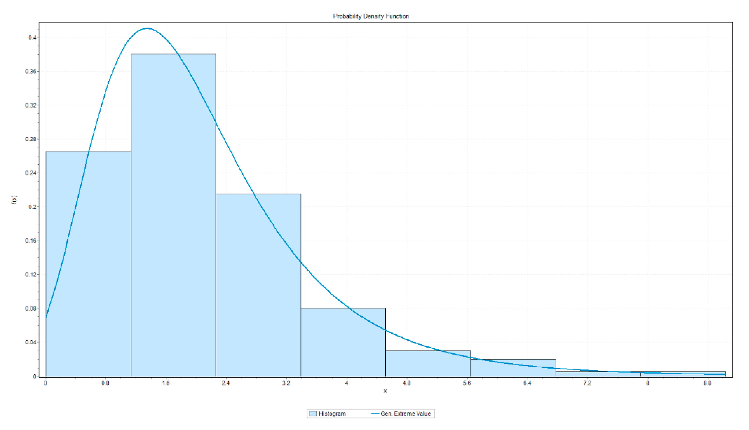
| Distribution | KS Statistics | Anderson–Darling Statistics |
|---|---|---|
| Gen. Extreme Values | 0.03253 (2) | 0.16401 (1) |
| Johnson SB | 0.03047 (1) | 0.19169 (2) |
| Gumbel Max | 0.05197 (3) | 0.4357 (3) |
| Logistic | 0.12206 (4) | 3.7302 (4) |
| Hypersecant | 0.1276 (5) | 4.0165 (5) |
| Normal | 0.12242 (6) | 4.0999 (6) |
| Anderson–Darling Statistics | |||||
| Sample Size | 200 | ||||
| Statistics | 0.16399 | ||||
| Rank | 1 | ||||
| α | 0.2 | 0.1 | 0.05 | 0.02 | 0.01 |
| Critical Value | 1.3749 | 1.9286 | 2.5018 | 3.2892 | 3.9074 |
| Kolmogorov–Smirnov Statistics | |||||
| Sample Size | 200 | ||||
| Statistics | 0.03251 | ||||
| P-Value | 0.97963 | ||||
| Rank | 2 | ||||
| α | 0.2 | 0.1 | 0.05 | 0.02 | 0.01 |
| Critical Value | 0.07587 | 0.08648 | 0.09603 | 0.10734 | 0.11519 |
| Study Site Algorithm | Sensitive Parameters | |
|---|---|---|
| Maccarese | Morris | Emergence, Senescence, Maturity, HIstart, Tbase, Tupp, Tmax_up, Tmax_lo, Tmin_up, Tmin_lo, GDD_up, GDD_lo, fshape_b, Zmax, CCmin, CCx, CDC, CGC, Kcb, fage, WP, WPy, HI0, HIini, exc |
| EFAST | CGC, HIstart, WP, HI0, Kcb, Emergence, Senescence, WPy, GDD_up, Maturity, fshape_b, Tmin_up, GDD_lo, CDC, PlantingDate, p_lo1, CN, MaxRooting, HIini, T_base, p_up2, Tupp, Tmax_up, b_HI, p_lo4, Flowering, CCmin, exc, HarvestDate, p_lo3, CCx, p_up4, REW, dHI_pre, fage, fsink, a_HI, fshape_w2, YldForm, SeedSize, Zmax, SxTopQ | |
| PAWN | CGC, HIstart, WP, Kcb, HI0, Senescence, WPy, Emergence, GDD_up, Maturity, Tmin_up, fshape_b, GDD_lo, CDC, b_HI | |
| Xiaotangshan | Morris | REW, Emergence, Senescence, Maturity, Histart, Tbase, Tupp, Tmin_up, Tmin_lo, GDD_up, GDD_lo, fshape_b, Zmax, CCmin, CCx, CDC, CGC, Kcb, fage, WP, WPy, HI0, exc |
| EFAST | CGC, Kcb, HIstart, WP, HI0, WPy, GDD_up, Maturity, Senescence, Emergence, Tmin_up, CDC, fshape_b,GDD_lo, HIini, CCmin, CN, Tbase, fshape_w4, Tmin_lo, MaxRooting, Zmax, CCx, fage, HI0, dHI_pre, Zmin, fshape_w2, REW, p_up4, HarvestDate, a_HI, p_lo3 | |
| PAWN | CGC, HIstart, WP, HI0, Kcb, Emergence, Maturity, Senescence, WPy, GDD_up, fshape_b, Tmin_up, GDD_lo, CCx, CCmin, fshape_w4, p_up4, p_up3, PlantingDate, HarvestDate, Tupp, p_up2, REW, Flowering, SeedSize, PlantPop, b_HI, dHI_pre, exc, Tmax_up, Tmin_lo, CDC, CN, dHI0, Tmax_lo, fshape_w2, YldForm, SxTopQ, fsink, HIini, Zmin, p_lo1, p_up1, Tbase, fshape_w1, p_lo4 | |
© 2020 by the authors. Licensee MDPI, Basel, Switzerland. This article is an open access article distributed under the terms and conditions of the Creative Commons Attribution (CC BY) license (http://creativecommons.org/licenses/by/4.0/).
Share and Cite
Upreti, D.; Pignatti, S.; Pascucci, S.; Tolomio, M.; Li, Z.; Huang, W.; Casa, R. A Comparison of Moment-Independent and Variance-Based Global Sensitivity Analysis Approaches for Wheat Yield Estimation with the Aquacrop-OS Model. Agronomy 2020, 10, 607. https://doi.org/10.3390/agronomy10040607
Upreti D, Pignatti S, Pascucci S, Tolomio M, Li Z, Huang W, Casa R. A Comparison of Moment-Independent and Variance-Based Global Sensitivity Analysis Approaches for Wheat Yield Estimation with the Aquacrop-OS Model. Agronomy. 2020; 10(4):607. https://doi.org/10.3390/agronomy10040607
Chicago/Turabian StyleUpreti, Deepak, Stefano Pignatti, Simone Pascucci, Massimo Tolomio, Zhenhai Li, Wenjiang Huang, and Raffaele Casa. 2020. "A Comparison of Moment-Independent and Variance-Based Global Sensitivity Analysis Approaches for Wheat Yield Estimation with the Aquacrop-OS Model" Agronomy 10, no. 4: 607. https://doi.org/10.3390/agronomy10040607
APA StyleUpreti, D., Pignatti, S., Pascucci, S., Tolomio, M., Li, Z., Huang, W., & Casa, R. (2020). A Comparison of Moment-Independent and Variance-Based Global Sensitivity Analysis Approaches for Wheat Yield Estimation with the Aquacrop-OS Model. Agronomy, 10(4), 607. https://doi.org/10.3390/agronomy10040607