Article

Prediction of Draft Force of a Chisel Cultivator Using Artificial Neural Networks and Its Comparison with Regression Model

by
Yousef Abbaspour-Gilandeh
1,*,
Masoud Fazeli
1,
Ali Roshanianfard
1,
Mario Hernández-Hernández
2,*,
Iván Gallardo-Bernal
3 and
José Luis Hernández-Hernández
4
1
Department of Biosystems Engineering, College of Agriculture and Natural Resources, University of Mohaghegh Ardabili, Ardabil 56199-11397, Iran
2
Faculty of Engineering, Autonomous University of Guerrero, Chilpancingo, Guerrero 39087, Mexico
3
Higher School of Government and Public Management, Autonomous University of Guerrero, Chilpancingo, Guerrero 39087, Mexico
4
Division of Research and Graduate Studies, TecNM/Technological Institute of Chilpancingo, Chilpancingo, Guerrero 39070, Mexico
*
Authors to whom correspondence should be addressed.
Agronomy 2020, 10(4), 451; https://doi.org/10.3390/agronomy10040451
Submission received: 9 February 2020 / Revised: 18 March 2020 / Accepted: 19 March 2020 / Published: 25 March 2020
(This article belongs to the Section Agricultural Biosystem and Biological Engineering)

Abstract

:
In this study, artificial neural networks (ANNs) were used to predict the draft force of a rigid tine chisel cultivator. The factorial experiment based on the randomized complete block design (RCBD) was used to obtain the required data and to determine the factors affecting the draft force. The draft force of the chisel cultivator was measured using a three-point hitch dynamometer and data were collected using a DT800 datalogger. A recurrent back-propagation multilayer network was selected to predict the draft force of the cultivator. The gradient descent algorithm with momentum, Levenberg–Marquardt algorithm, and scaled conjugate gradient descent algorithm were used for network training. The tangent sigmoid transfer function was the activation functions in the layers. The draft force was predicted based on the tillage depth, soil moisture content, soil cone index, and forward speed. The results showed that the developed ANNs with two hidden layers (24 and 26 neurons in the first and second layers, respectively) with the use of the scaled conjugate gradient descent algorithm outperformed the networks developed with other algorithms. The average simulation accuracy and the correlation coefficient for the prediction of draft force of a chisel cultivator were 99.83% and 0.9445, respectively. The linear regression model had a much lower accuracy and correlation coefficient for predicting the draft force compared to the ANNs.

1. Introduction

The optimization of agricultural equipment is an important strategy to improve tool performance, production efficiency, and cultivation outcomes as well as to cope with the food shortage and growing population. Predicting the related parameters of implements can improve the quality of field work and increase their efficiency. Cultivators, as agricultural equipment, are applied for various purposes such as weed control [1,2]. The use of cultivators is still one of the most cost-efficient and applicable method. These tools are considered by farmers to promote plant growth through weed control, soil preparation, soil permeability modification to irrigation, mixing of chemical fertilizers and insecticides with soil, providing protection for plants, and increased activity of microorganisms [1,3]. Despite much work being done to control the weeds in agricultural ecosystems, they incur severe damage to the crops. Weed control is one of the most costly measures taken to increase the crop quality and has direct effects on the product price [4].
Many studies have shown that tillage equipment often requires a high amount of energy to perform during operations, and the optimal management of this energy will help to decrease fuel consumption and costs [3,4,5,6,7,8]. In this regard, an appropriate selection of the tractor and equipment are required. It is possible to predict the required draft force, identification of the tractor traction capacity, and total energy required for the equipment transportation. Thus, agricultural machinery engineers select the most suitable tractor power with the knowledge of the draft force and power required in different soils [4].
Regarding the use of cultivators for weeding, Biswas et al. (2000) developed the optimum shape of a cultivator blade for animal-drawn weeders [9]. They evaluated four types of blades (straight, triangular, curved, and sweep blades) in terms of the required draft force. Their study showed that the flat sweep type requires the minimum draft force and could also improve weed penetration and cutting.
Concerning the use of powerful design software to analyze the forces applied to the cultivator, Ahmadi-Moghaddam and Komarizadeh [8] analyzed two types of cultivator shank (spring and rigid) with sweep and chisel blades in ANSYS software (ANSYS Inc., Canonsburg, PA, USA). The results showed that the stresses in the fixed shanks were greater than the spring shanks, but the deformation in the spring shanks was more than that of the fixed shanks. Nasiri (2010) also applied the finite element method to determine the draft force of the cultivator [7]. They used the ABAQUS software (ABAQUS Inc., Pawtucket, RI, USA) to simulate the cultivator–soil interaction. The results showed that the draft force reached certain values after some fluctuation, which was much lower than the values obtained from the Hendrick method [10]. This was due to the difference between the soil texture and soil conditions. Based on Nasiri’s report, Hendrick’s experiment was conducted on hard soils, which require a large draft force [7,10]. In general, the finite element results showed higher values than Safdari’s (2008) results, but in some points, the field results were more reliable than the finite element results, which may be due to the presence of rocks, clods, local compaction of soil, or roots of plants [11]. The finite element results were found to be more similar to the results of Safari’s (2008) experiments [2].
The forward speed of tools, soil moisture content, and soil cone index are among the important parameters that influence the draft force of the cultivators. Hendrick (1988) obtained the draft force of chisel plows and field cultivators in the hard soil when the blades were working at the depth of 8.26 cm and forward speed of 1.5–3 m/s. The results for the loamy, loamy-clayey, and clayey soils reported as 520 + 49.2S, 480 + 48.1S, and 527 + 36.1S, respectively (S is tool speed in m/s) [10]. Safdari [12] performed the mechanical and dynamic analysis of the cultivator shank using the finite element method. For this purpose, the draft force applied to the cultivator shank was measured at three speeds of 0.88, 1.6, and 2.5 m/s at a 15 cm depth and then the force–time diagram was plotted. The results of this measurement showed that the average draft force at the speeds of 0.88, 1.6, and 2.5 m/s were 234.77, 325, and 655.05 N, respectively. The results showed an increase in force as the velocity was increased.
Abbaspour-Gilandeh et al. (2012) conducted the experiments on a 16-hectare soybean field located in the Moghan Plain in the Ardabil Province of Iran to evaluate a high-speed row cultivator and compare its performance with a crescent cultivator. Based on the evaluation data, it was found that by increasing the forward speed, the high-speed cultivator tended to slightly decrease the depth, which indicates that the machine is well capable of maintaining the working depth at high speeds and can operate at 10.2 km/h. After the operation of the row cultivator with high forward speed, all weeds across the blade cut were cut and removed from the depth of 5–7 cm. In the crescent cultivator, however, due to the concave structure of the blade, the weeding depth was not uniform and was about 2–3 cm in the sides. In the row cultivator with high forward speed, 60% of the plants were partially damaged by the plates through the leaf, and the blade damage to the main plant was zero. The results of the analysis of variance showed no significant difference between the two machines in both the forward speeds in terms of the impact on the soil bulk density. In terms of the impact on the soil moisture at the depth of 1–10 cm, there was only a significant difference at the 5% probability level between both forward speeds. Based on these results, the cultivator with flat sweep blades (row cultivator with high forward speed) showed good performance and can be used in row crops such as corn, soybean, cotton, and sunflower. It can also be equipped with a fertilizer drill unit or a row sprayer and can perform fertilization, spraying, and weeding operations with high field capacity in a single run [5].
Computer models help researchers to predict the draft of tillage tools such as cultivators without conducting expensive as well as time-consuming field tests. They also help researchers and manufacturers to improve the tool design by comparing and analyzing various parameters that influence the tool draft [12,13]. Due to non-linear and stochastic features of soil–tool interactions, artificial intelligence approaches like artificial neural networks (ANNs) have been employed for estimating the performance parameters of soil working machines. The ANNs are a set of nonlinear connected processing elements that consist of single processing elements with a large number of inputs and outputs, and work in three stages including training, the validation and test process, and the application [14,15,16]. Due to the limitations of the linear regression methods for function approximation, the ANNs can be a useful method to predict the required energy of tillage using different parameters of soil and speed data. This is the reason for using this method, as the values of the input and output parameters are linked without any predetermined hypothesis or mathematical relation. In such cases, where insufficient information is available on the relationships between the parameters, the ANN acts as a powerful tool in modeling the soil system. Askari and Abbaspour-Gilandeh (2019) investigated the ability of the adaptive neuro-fuzzy inference system (ANFIS) and response surface methodology (RSM) approaches for predicting the draft force of subsoiling tines. The results showed that the ANFIS model presented better accuracy than the RSM and regression models to predict the draft force with a mean squared error (MSE) of 0.0156 and R2 of 0.998 [14].
However, due to the importance of this topic and the difficulties of comprehensive research, it seems necessary to further address and evaluate the research in this field. In general, the objectives of this research can be stated as follows:
  • Prediction of the draft force of the chisel cultivator with the ANN model using the physical and mechanical properties of soil, tractor speed, and working depth.
  • Comparison of the accuracy of different artificial neural network training methods to predict the required draft force of the chisel cultivator.
  • Comparison of the accuracy of the ANN model with the linear regression model in order to predict the draft force of the chisel cultivator.

2. Materials and Methods

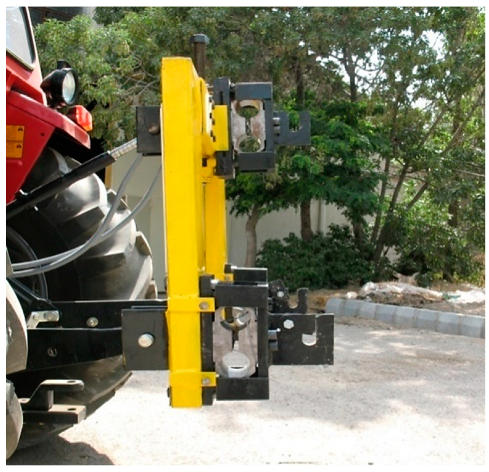
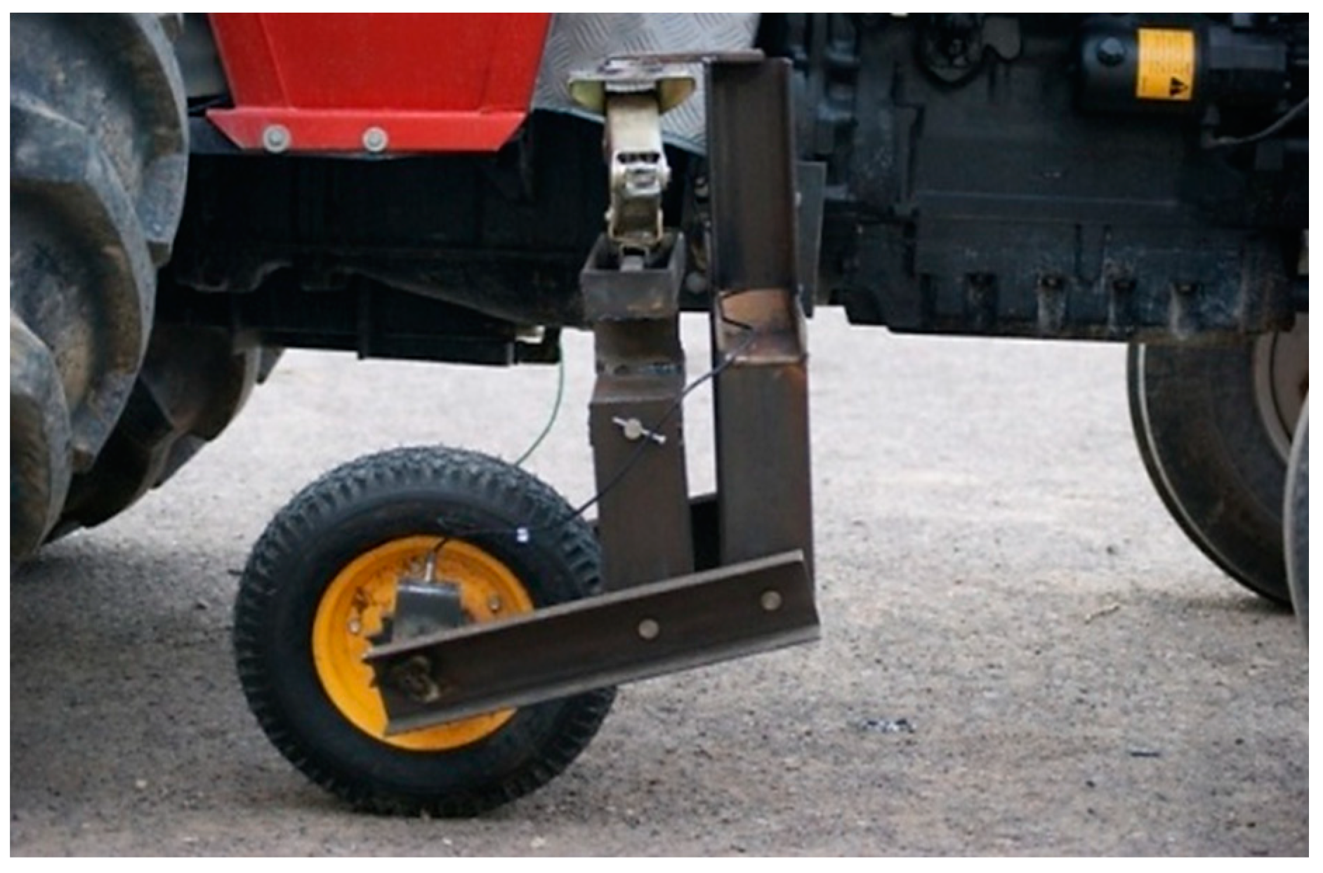
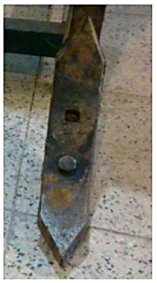
2.1. Equipment Used for Experiments

In this study, the draft force required for the field experiments was provided by a 75 hp rear-axle MF-285 Massey Ferguson tractor (ITMCO, Tabriz, Iran). The tractor was equipped with precision measuring systems to collect the draft force, forward speed, and dynamic load data applied on the front wheels during the tillage operation. The tools included a three-point hitch dynamometer, a fifth wheel speed sensor, a dynamic load measuring sensor (strain gauges mounted on the front axle of the tractor), a laptop computer, and a data collection system (DT800 data logger, Omni instruments Ltd., Dundee, Scotland, UK). The following will describe the structure and operation of some of the equipment [17].

2.2. Draft Force and Actual Tractor Speed Measurement System

The dynamometer used in this study (Figure 1) was a three-point adjustable hitch dynamometer designed and constructed at the University of Mohaghegh Ardabili [18]. The total draft force required to pull the tillage tool into the soil ( F t o t a l ) is calculated by Equation (1):
F t o t a l = F R X + F L X F T X
where F R X , F L X , and F T X are the horizontal forces applied to the right lower, left lower, and upper hitch pins, respectively.
Additionally, to obtain the energy required for tillage operation, Equation (2) was used:
E = E P T O × t
where E is the required energy ( k W . h ); t is the time required to perform the tillage operation within the test plot ( h ); and E P T O is the equivalent power consumption of the tractor power take-off for the tillage operation ( kW ).
In this research, a fifth wheel (Figure 2) consisting of a 39   cm diameter rubber wheel, a mechanical jack for height control, an encoder for rotation counting, and a pulse meter for rotation measurement was used to measure the forward speed of the tractor.
In the field experiments, to compare the draft force and required energy of conventional cultivators in the weeding operation, a cultivator with a chisel blade and C-shaped spring shank (Figure 3) was used.
In order to measure the soil cone index values in the test plots, a cone penetrometer (Figure 4) was mounted behind the tractor. The penetrometer was mounted to the three-point hitch of a tractor, which was equipped with multiple penetration rods that could measure the soil cone index values at various points and depths [19]. The main part of the penetrometer is a cone-shaped end-tool with a cross-section of 133 mm2 and a 30 ° point angle, which was added to the end of a 95 cm long rod. The rod attached to the cone tip was pushed into the soil using the hydraulic force generated by the hydraulic jack.
A soil profile meter device that was 75 cm long and 60 cm wide with parallel vertical bars in a 5 cm spacing was used to investigate the soil disturbance caused by the cultivators during the tests. Prior to the tillage operation by cultivators, a soil sample was taken from each test section and three replications were taken to measure the moisture content. The samples were then transferred to the laboratory to determine the moisture content. The samples were weighed in the laboratory with an electronic sensitive scale and then placed in an oven at 105 °C for 24 h. After 24 h and re-weighing the soil samples, the soil moisture content (based on dry weight) was determined.

2.3. Field Experiments

The field experiments were performed in the educational and research field of the Agriculture Faculty in the University of Mohaghegh Ardebili with loamy sandy soil. In this study, the factorial test based on the randomized complete block design (RCBD) with three replications was used to measure and determine the factors affecting the amount of draft force, energy, and soil disturbance of each cultivator. In the tested soil, different moisture levels (factor A) from 5 to 16% for dry soils and 17 to 35% for wet soils (measured after 24 h after irrigation), tractor forward speed (factor B) at four levels, working depth (factor C) at two levels of 10 and 20 cm within each test plot, draft force of cultivators with different blades, soil cone index, and soil moisture content were measured. The cone index values were measured in each test plot after identifying the field and bounding by wooden nails and applying the moisture conditions. The cone index values in each test plot were measured at three points for each location from 0 to 40 cm in depth.
After measuring the soil cone index values, by removing the cone index tool and preparing and attaching the cultivators and measuring instruments inside the tractor cabin, the work to measure the draft force was undertaken. The depth required for the cultivators was adjusted by the lower links of the tractor and the gauge wheels. Then, by selecting the predicted gear and engine rotation, the data capture and the record of output signals from the circuit was begun. The movement was carried out for 30 m and then returned at the end of the field, and the experiment with the next conditions was performed with a 1.5 m distance from the previous furrow. For each condition, 40 furrows were created inside the soil. The data obtained at the end of each furrow was saved in a separate .txt file. In order to apply the moisture conditions, the test land was irrigated to achieve the desired moisture range.

2.4. Prediction of Draft Force of Cultivator with Chisel Blade Using ANNs

2.4.1. Artificial Neural Network (ANN) Model Design

In this research, MATLAB R2008a (The MathWorks Inc., Natick, MA, USA) was used to develop the ANN model to predict the draft force of the cultivator with a chisel blade. This software has surpassed other software available in this field and has been widely used in various fields by having powerful functions in the area of ANNs. The following sections discuss the design of ANNs in terms of training methods, the number of neurons in the layers, and the network parameter selection.

2.4.2. Network Type and Training Method

The ANNs designed in this study were multilayer back-propagation multilayer networks. Many studies performed for prediction works have used the scaled conjugate gradient, gradient descent with momentum, and Levenberg–Marquardt algorithms [16]. The gradient descent algorithm is time-consuming due to the need for a lower learning rate to achieve stable training. The gradient descent with momentum is a much faster algorithm because it uses a higher learning rate to achieve stability. In general, the use of the Levenberg–Marquardt training algorithm for a medium-sized network is recommended. The scaled conjugate gradient algorithm (similar to the Levenberg–Marquardt training algorithm), is one of the fastest training algorithms in MATLAB. In this research, three methods of gradient descent with momentum, Levenberg–Marquardt, and scaled conjugate gradient algorithms were used to train the network, as shown in Figure 5. The most important factor in the design of ANNs is the selection of data used as the training data and testing data. In this research, the input parameters were: (1) the soil moisture content; (2) forward speed of tractor; (3) soil cone index; and (4) blade penetration depth. The draft force of the chisel cultivator is the output parameter of the designed network. To train the designed network and test the network, the collected data were divided into three separate files: 50% of the total data were used for network training, 25% for network validation, and 25% for network testing.

2.4.3. Learning Parameters

In the error back-propagation networks, it is very important to select the correct learning rate to achieve a convergence. The learning rate (LR) determines the length of steps for each weight correction and the biases of the network. A simple way to increase and improve the LR is to add a parameter called momentum (M) to the network. The M is part of the weight change made in the prior iteration. For each learning parameters including the LR and the M, the initial values of 0.3 and 0.4 were considered, respectively [16,20].

2.4.4. Number of Neurons and Activation Functions

Multilayer networks are beneficial for prediction applications if they have enough neurons in the hidden layer. The multilayer networks are susceptible to the number of neurons in the hidden layer(s). The low number of neurons causes mismatch and the high number of neurons causes overfitting, and the network may lose the generalization capability. Minimizing the number of neurons in a hidden layer without affecting the network performance is one of the important criteria in network design. Selecting the number of intermediate-layer neurons is a trial-and-error process as it is not possible to make general comments on the number of hidden layers and to select the appropriate number of hidden-layer neurons. Therefore, in this study, the number of hidden layers and the number of neurons in the intermediate layer were selected based on the comparison of the network performance according to the number of intermediate-layer neurons. The differentiability of the transfer function in each neuron is the only limiting factor for the selection of the functions in the recurrent back-propagation networks. Most research has used the sigmoid function as the transfer function of network neurons [14,15,16,20]. In this study, the hyperbolic tangent, sigmoid, and linear activation functions were used between the network layers.

2.4.5. Normalization

The sigmoid function is one of the most commonly used activation functions in the ANN structure, which ranges all binary numbers. Therefore, there is no limit to the use of this function in terms of network input data. To prevent the network from the early stop and early saturation of neurons, normalization of the data is a useful method. Normalization is the placing of data in the sigmoid linear range and limiting them to the range of (0,1). To normalize the data, the standard deviation, mean of the data, and the subtraction of each data from the mean were calculated, and then the calculated values were divided by the standard deviation of the data.

2.4.6. Network Performance Evaluation

One of the most important steps to test and validate a method is the evaluation of its performance and efficiency. To develop an ANN model, it is important to evaluate the network performance and accuracy. It is also better to have the accuracy of models in order to compare different models with each other. This section covers the methods used for evaluating the performance of networks and their comparison in this study.

Dot Chart

An appropriate way to evaluate the network performance and other models is to plot the predicted values of the model against the actual values in a chart. Matching the points plotted on the bisector line of the first and third quadrants is the most appropriate state. This chart is not suitable for comparing multiple charts and is mostly a qualitative chart. Therefore, the quantitative indicators should also be used to compare and evaluate the models.

Quantitative Indicators

One of the most commonly used quantitative indicators for evaluating the network and various models is the correlation coefficient (R) expressed by Equation (3):
R = i = 1 n ( X i X ¯ ) ( Y i Y ¯ ) i = 1 n ( X i X ¯ ) 2 . i = 1 n ( Y i Y ¯ ) 2         1 < R < 1
where X i is the predicted values; Y i is the actual values; X ¯ is the mean of the predicted values; and Y ¯ is the mean of the observed values. From the correlation coefficient, another coefficient is defined, called the model coefficient of determination (R2).
The mean squared error (MSE) is another quantitative indicator used to estimate the accuracy of the artificial neural network model and other various models, which evaluates the accuracy of the model based on the difference between the actual and the predicted values. The MSE is obtained from Equation (4):
M S E = 1 n i = 1 n ( P i A i ) 2
where n is the number of iterations; Pi is the predicted value; and Ai is the actual value. Since, the R2 value (model coefficient of determination) approaches one when the MSE value approaches zero, it is found that the lower the MSE value, the better the model performance. Another quantitative indicator is the sum of squared errors (SSE) and its only difference with the MSE is that the mean squared error is calculated in the MSE, but the sum of squared error is calculated in the SSE rather than the mean.
For the statistical comparison of the accuracy of the designed networks, a measure called model prediction accuracy is used. The prediction accuracy (PA) of the model is expressed using Equation (5):
P A = ( 1 1 n i = 1 n | A i P i | A i ) × 100
where n is the number of observations; Pi is the predicted value; and Ai is the actual value.

3. Results and Discussion

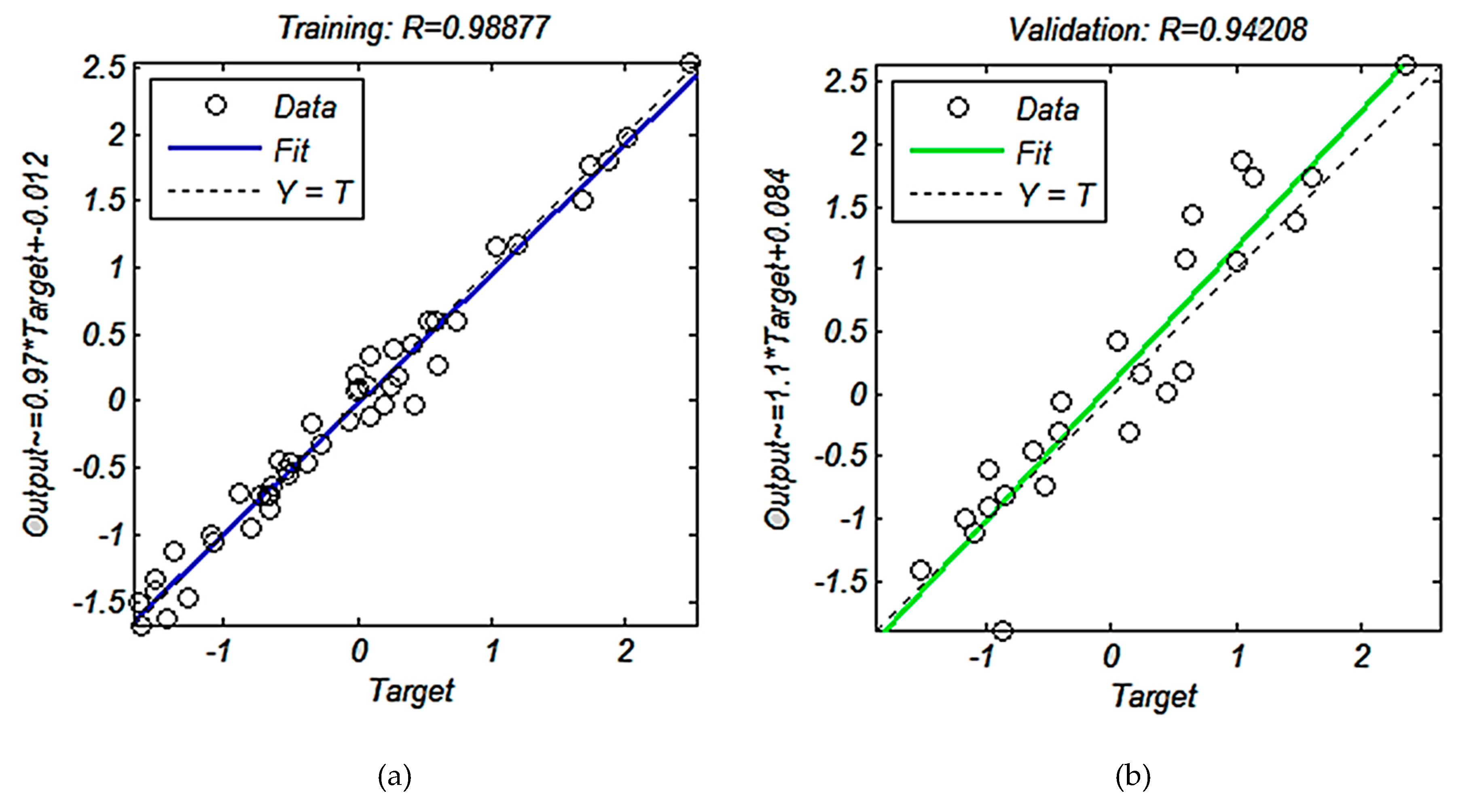
3.1. Prediction of Draft Force Using ANNs

In this study, the three training algorithms of gradient descent with momentum, Levenberg–Marquardt, and scaled conjugate gradient were used to train the ANNs. The minimum value set for the network MSE was 0.01. Selection of the appropriate number of hidden layers and the number of neurons in the hidden layers was performed based on the comparison of the performance of networks with the different number of neurons in the hidden layer. Table 1, Table 2 and Table 3 present the results of the networks designed to predict the draft force of the cultivator using the mentioned training methods with the different intermediate layer(s) and the number of neurons in the hidden layer. The activation function used between the intermediate layers is the sigmoid tangent function. According to Table 3, it can be stated that a network with two layers in the hidden layer (24 neurons in the first and 26 neurons in the second layer), was found to be suitable for predicting the draft force. The network had good values of the mean, MSE, and coefficients of determination of the network during the training, evaluation, and testing stages. The network has the coefficients of determination of 0.826004, 0.767925, and 0.788527 for the training, evaluation, and testing stages, respectively, which had the most appropriate values compared to other topologies. Similar tables were obtained for the other mentioned training algorithms by changing the number of hidden layers (at most two hidden layers) and changing the number of neurons in the hidden layers, similar to that in Table 3.
After the network was trained (in each algorithm and for every number of hidden neurons), a chart was obtained in MATLAB software, which showed the variations in the error of the network’s training, validation, and testing. Figure 6 shows an example of the charts illustrated for the error changes in the training, evaluation, and testing data in a designed sample network. As illustrated in Figure 6, the training algorithm was terminated when the training error was small enough, and the test and validation error showed similar characteristics.
Figure 7 shows the MSE chart in terms of the epoch, which was used to better and more precisely control the network training process and investigate the overfitting phenomenon. For each iteration, there was an SSE that was used to represent the changes as a criterion for understanding the network performance. The blue, green, and red lines represent the error variations for the training, evaluation, and testing data, respectively, and the black line represents the target error value of the network. Using a network with two intermediate layers and 24 neurons in the first layer and 26 neurons in the second intermediate layer, the MSE in the 21st cycle was 0.0398.
Figure 8 is a chart showing the line of best fit between the actual (T) and predicted values by the network (Y). The network developed with two hidden layers and 24 neurons in the first layer and 26 neurons in the second layer had the highest slope, lowest ordinate, and highest correlation coefficient with the values of 1, 0.2, and 0.9445, respectively. The red line corresponds to the line of best fit among the data points, and the black dotted line is the bisector of the first quadrant of two vertical and horizontal axes. The closer fitted line to the bisector line is the better fitting and more accurate for the estimation of the network outputs. Due to a large number of charts, only the charts of the scaled conjugate gradient (trainscg) algorithm with 24 neurons in the first layer and 26 neurons in the second layer are provided. The regression charts for the training, evaluation, testing, and overall stages are separately shown in Figure 9. The highest correlation coefficient was 0.9888 for the training stage. The correlation coefficients of evaluation and testing stages were 0.9421 and 0.8993, respectively.
In order to compare the three training algorithms and to compare the accuracy and statistical parameter obtained for the networks, the results are shown in Table 4. This table presents the training algorithms used, network structure, network correlation coefficients, and average simulation accuracy. Additionally, the learning and momentum rate of 0.3 and the linear transfer function in the output layer were used in each network. According to Table 4, it can be stated that the network designed with the scaled conjugate algorithm with 24 neurons in the first layer and 26 neurons in the second layer had the highest value of simulation accuracy and correlation coefficient.

3.2. Comparison of ANN Model with the Linear Regression Model

In order to evaluate and compare the performance of ANNs with the linear regression model, the data from the two models were compared to predict the draft force of the chisel cultivator. SPSS 19 software was used to obtain the linear regression model. The parameters included in the model were the soil moisture content, forward speed, working depth, soil cone index, and draft force. In the linear regression model, the first four parameters were considered as independent variables and the draft force parameter as the dependent variable. The correlation coefficient and prediction accuracy for the linear regression model were 0.592 and 61%, respectively, which were significantly lower than the correlation coefficient and prediction accuracy of the ANN model, which were 0.9445 and 89%, respectively. The results are in agreement with those obtained by Al-Janobi and Al-Suhaibani (1998) and Alimardani et al. (2009) [4,13]. Equation (6) shows the linear regression equation obtained from the experimental data:
F = 81.305   D 3.799   S 113.384   R 28.781   C + 265.272
where F is the draft force ( Kgf ); D is the working depth (cm); R is the moisture content; C is the soil cone index (MPa); and S is the forward speed (km/h).
The comparison of the results obtained from the ANN model and linear regression model to predict the draft force of the chisel cultivator showed that the predicted data by those two models were in the range presented by the ASABE model [12]. However, the ASABE model presents an accuracy of ±50% in the prediction of the draft force. The ANN model gave predicted data very close to the actual data compared to the results obtained from other models such as the ASABE model and linear regression model.

4. Conclusions

Most of the research on the draft force of tillage tools has been focused on measuring the draft force and developing draft prediction models using regression and artificial intelligence models. In this study, the multilayer recurrent back-propagation artificial neural networks were used to predict the draft force of the cultivator with a chisel blade. The input parameters of the ANNs were the soil moisture content, forward speed of tractor, soil cone index, and working depth. The draft force of the chisel cultivator was the output parameter of the designed network. In order to train the network, three types of algorithms were used: the gradient descent with momentum, scaled conjugate gradient, and Levenberg–Marquardt. The results showed that the scaled conjugate gradient algorithm with two hidden layers and 24 neurons in the first layer and 26 neurons in the second layer had the highest simulation accuracy of 89.48% and correlation coefficient of 0.9445 compared to the other training algorithms. The correlation coefficient and prediction accuracy for the linear regression model were 0.592 and 61%, respectively, which were significantly lower than the correlation coefficient and prediction accuracy of the neural network. Therefore, the model developed in this paper is useful for predicting the draft force of a chisel cultivator and designing a chisel cultivator with low draft force. It is proposed that experiments be undertaken at several soil textures, different soil moisture contents, and at different soil compactness in order to develop a model with high accuracy and high generalizability.

Author Contributions

Conceptualization, Y.A.-G. and M.F.; Methodology, Y.A.-G., M.F.; Software, Y.A.-G., M.F., and A.R.; Validation, Y.A.-G., and M.H.-H.; Formal analysis, M.F., Y.A.-G., and A.R.; Investigation, Y.A.-G. and M.F.; Resources, Y.A.-G. and M.F.; Data curation, M.F.; Writing—original draft preparation, M.F. and A.R.; Writing—review and editing, Y.A.-G., M.H.-H., I.G.-B., and J.L.H.-H.; Visualization, Y.A.-G. and A.R.; Supervision, Y.A.-G.; Project administration, Y.A.-G.; Funding acquisition, Y.A.-G., M.H.-H., I.G.-B., and J.L.H.-H. All authors have read and agree to the published version of the manuscript.

Funding

This study was financially supported by the University of Mohaghegh Ardabili.

Conflicts of Interest

The authors declare no conflicts of interest. The funders had no role in the design of the study; in the collection, analyses, or interpretation of data; in the writing of the manuscript, or in the decision to publish the results.

References

  1. Jabran, K.; Chauhan, B.S. Non-Chemical Weed Control; Academic Press: Cambridge, MA, USA, 2018. [Google Scholar]
  2. Safari, M. Design, Manufacture and Evaluation of Rotary Cultivator; Institute of Agricultural Engineering and Engineering Research: Karaj, Iran, 2008. [Google Scholar]
  3. Bell, B. Farm Machinery; Old Pond Books: West Sussex, UK, 2010. [Google Scholar]
  4. Al-Janobi, A.; Al-Suhaibani, S. Draft of primary tillage implements in sandy loam soil. Appl. Eng. Agric. 1998, 14, 343–348. [Google Scholar] [CrossRef]
  5. Abbaspour, Y.; Bavafa, M. Design and construction of a high speed inter-row cultivator. Appl. Mech. Mater. Vols 2011, 110, 4914–4918. [Google Scholar] [CrossRef]
  6. Abbaspour-Gilandeh, Y.; Khalilian, A.; Reza, A.; Alireza, K.; Sadati, S. Energy savings with variable-depth tillage. In Proceedings of the 27th Southern Conservation Tillage Systems Conference, Florence, SC, USA, 27–29 June 2005; pp. 84–91. [Google Scholar]
  7. Nasiri, M. Calculation of required draft force of cultivator using 3D finit element methods. In Proceedings of the 6th National Congress of Agriculture Machinary, Karaj, Iran, 15–16 September 2010. [Google Scholar]
  8. Ahmadi-Moghaddam, P.; Komarizadeh, M.H. Simulation of Cultivator Shank with ANSYS. In Proceedings of the Second National Congress of Agricultural Machiney and Mechanization, Tehran, Iran, 30–31 October 2002. [Google Scholar]
  9. Biswas, H.; Rajput, D.; Devnani, R. Animal-Drawn Weeders for Weed Control in India; Atnesa: Wageningen, The Netherlands, 2000; pp. 134–140. [Google Scholar]
  10. Brown, R. Handbook of Engineering in Agriculture; CRC Press: Boca Raton, FL, USA, 1988; Volume I. [Google Scholar]
  11. Safdari, S. Dynamic and Mechanical Analysis of Cultivator Shank Using Finite Element Methods; Agricultural Machinery Department, Urmia University: Urmia, Iran, 2008. [Google Scholar]
  12. Agricultural, A.S.O.; Engineers, B. Agricultural Machinery Management Data; American Society of Agricultural and Biological Engineers: San Jose, MI, USA, 2011. [Google Scholar]
  13. Alimardani, R.; Abbaspour-Gilandeh, Y.; Khalilian, A.; Keyhani, A.; Sadati, S.H. Prediction of draft force and energy of subsoiling operation using ANN model. J. Food Agric. Environ. 2009, 7, 537–542. [Google Scholar]
  14. Askari, M.; Abbaspour-Gilandeh, Y. Assessment of adaptive neuro-fuzzy inference system and response surface methodology approaches in draft force prediction of subsoiling tines. Soil Tillage Res. 2019, 194, 104338. [Google Scholar] [CrossRef]
  15. Mansourian, S.; Darbandi, E.I.; Mohassel, M.H.R.; Rastgoo, M.; Kanouni, H. Comparison of artificial neural networks and logistic regression as potential methods for predicting weed populations on dryland chickpea and winter wheat fields of Kurdistan province, Iran. Crop Prot. 2017, 93, 43–51. [Google Scholar] [CrossRef]
  16. Suzuki, K. Artificial Neural Networks: Architectures and Applications; InTech Publisher: Rijeka, Croatia, 2013. [Google Scholar]
  17. Abbaspour-Gilandeh, Y.; Rashidi-Mohammadabad, F. Evaluation of dynamic load equations through continuous measurement of some tractor tractive performance parameters. Int. J. Heavy Veh. Syst. 2013, 20, 222–235. [Google Scholar] [CrossRef]
  18. Abbaspour-Gilandeh, Y.; Haghighat-Shishvan, S. Extended octagonal ring transducers for measurement of tractor-implement forces. Instrum. Exp. Tech. 2011, 54, 136–140. [Google Scholar] [CrossRef]
  19. Abbaspour-Gilandeh, Y.; Ahani, M.; Askari Asli-Ardeh, E.; Rasooli-Sharabiani, V.; Sofalian, O. Design, fabrication and evaluation of a tractor-mounted soil cone penetrometer with multiple probes. J. Agric. Eng. Res. (Iran) 2010, 11, 19–34. [Google Scholar]
  20. Rahimi-Ajdadi, F.; Abbaspour-Gilandeh, Y. Artificial neural network and stepwise multiple range regression methods for prediction of tractor fuel consumption. Measurement 2011, 44, 2104–2111. [Google Scholar] [CrossRef]
Figure 1. Adjustable three-point hitch dynamometer for measuring the draft force of implements.
Agronomy 10 00451 g001
Figure 2. Adjustable fifth-wheel to measure the forward speed of the tractor.
Agronomy 10 00451 g002
Figure 3. Chisel cultivator blade used in the research.
Agronomy 10 00451 g003
Figure 4. Tractor-mounted soil cone penetrometer for measuring the soil cone index.
Agronomy 10 00451 g004
Figure 5. The artificial neural network (ANN) used in this study.
Agronomy 10 00451 g005
Figure 6. The training, validation, and testing errors versus the number of epochs (iterations).
Agronomy 10 00451 g006
Figure 7. Network performance charts of the scaled conjugate gradient with two intermediate layers and 24 neurons in the first layer and 26 neurons in the second layer.
Agronomy 10 00451 g007
Figure 8. Network regression chart with 24 neurons in the first layer and 26 neurons in the second layer.
Agronomy 10 00451 g008
Figure 9. Network regression chart for the (a) training, (b) evaluation, (c) testing, and (d) overall stages.
Agronomy 10 00451 g009aAgronomy 10 00451 g009b
Table 1. Quantitative indicators for evaluating networks developed using the Levenberg–Marquardt algorithm.
Number of NeuronsLRMMSECoefficient of DeterminationAverage Accuracy of Network (%)Correlation Coefficient
TestValidationTrain
4 + 20.30.30.09040.7805270.7771650.77443383.660.9101
4 + 60.30.30.08960.8014910.7570880.79603183.250.9115
6 + 60.30.30.09050.7718850.7241200.73476684.430.9094
8 + 80.30.30.04380.8757790.7246490.65242183.840.8856
10 + 80.30.30.15900.7558570.7730740.74582483.650.8907
12 + 100.30.30.04660.9034610.7321010.71711084.350.9108
12 + 120.30.30.01470.9331350.7832730.68728283.830.8930
12 + 140.30.30.14800.7322160.7875840.58385981.750.8717
16 + 140.30.30.07930.8342140.7677700.71917783.660.9039
16 + 160.30.30.01310.9428640.6582600.67552983.860.8776
22 + 200.30.30.05340.8721060.7432750.70571681.500.8971
22 + 240.30.30.03460.8709370.7022340.62389283.980.8877
26 + 240.30.30.00340.9765610.7381810.69962685.070.9292
28 + 280.30.30.05270.8832260.6575560.75312983.670.9114
36 + 340.30.30.04770.8648710.7353060.62753784.850.8764
36 + 360.30.30.05880.8463730.7243300.66102982.540.8873
38 + 400.30.30.01430.9407120.7256930.66828983.900.8864
Table 2. Quantitative indicators for evaluating networks developed using gradient descent with momentum algorithm.
Number of NeuronsLRMMSECoefficient of DeterminationAverage Accuracy of Network (%)Correlation Coefficient
TestValidationTrain
6 + 40.30.30.1510.7565920.7501690.77422684.490.8897
6 + 60.30.30.07820.8387320.7751750.792586.020.9223
8 + 60.30.30.1050.7916110.7384370.747683.450.8881
10 + 100.30.30.1070.7936640.7555170.71516484.40.8921
10 + 120.30.30.120.7823860.7723130.76738383.730.8945
12 + 120.30.30.09730.8330130.7912570.76808485.470.9102
Table 3. Quantitative indicators for evaluating networks developed using scaled conjugate gradient algorithm.
Number of NeuronsLRMMSECoefficient of DeterminationAverage Accuracy of Network (%)Correlation Coefficient
TestValidationTrain
4 + 40.30.30.1150.7787410.7660890.77043184.970.9089
6 + 40.30.30.1480.7749820.7858520.79940585.470.9113
6 + 60.30.30.1260.8214940.812120.77299484.200.8979
8 + 60.30.30.04670.8649550.7577320.67838285.360.9017
10 + 100.30.30.08890.8225350.7843210.68670283.730.891
12 + 100.30.30.08690.8404820.75980.74034185.040.9064
14 + 120.30.30.09660.7978440.7907390.78484885.270.9089
16 + 140.30.30.6670.8552650.7853720.74082385.720.9171
16 + 180.30.30.06850.8447450.7560350.6969584.250.8918
20 + 180.30.30.09640.8280550.7821760.75142185.180.9094
20 + 200.30.30.03720.8950460.8312870.7912788.530.9403
22 + 200.30.30.03080.9048660.8209770.80846287.140.9255
22 + 240.30.30.02740.9115220.762560.71644985.840.8916
26 + 240.30.30.08450.8260040.7679250.78852789.480.9445
26 + 280.30.30.02560.9161370.7569230.68418586.420.9017
28 + 280.30.30.02990.90450.8065090.75862687.140.9257
34 + 320.30.30.06250.8479210.7460240.68565184.650.8983
34 + 360.30.30.03350.884060.816230.71177486.400.9042
38 + 360.30.30.04150.8868070.7180520.64831185.770.9197
38 + 400.30.30.03620.8958070.7627680.78285286.220.908
40 + 400.30.30.02550.9132830.7409690.76407586.860.9172
Table 4. Networks designed using three training algorithms with an optimal number of neurons in the hidden layer.
Training AlgorithmActivation FunctionNumber of Neurons in Hidden LayerEpochMSEAverage Accuracy of Network (%)Correlation Coefficient
Trainlmtansig26 + 2430.0033585.070.9292
Traingdmtansig6 + 6550.078286.020.9223
Trainscgtansig26 + 24210.039889.480.9445

