Risk Management Tools for Sustainable Agriculture: A Model for Calculating the Average Price for the Season in Revenue Insurance for Citrus Fruit

Abstract

Risk management in agriculture is at the heart of major reforms in many OECD countries and European agricultural policies. Price risks, which are generally not insurable per se, have been covered by the Common Agricultural Policy (CAP), which has been shaped as a system of protection against market shocks and an instrument for income stabilization. However, there is an increasing propensity to combine the use of public and private risk management tools as well. In Spain, revenue insurance has not yet developed in the same way as other risk coverage insurance, although it is an upcoming target of agricultural insurance policies with the aim of ensuring income stability for agricultural producers. This paper presents the results of the methodology used to draw up a composition index or model of the average price for the season or representative market field price to be used for revenue insurance purposes in citrus fruit. High explanatory power regression models and the analytic hierarchy process (AHP) were used. The results show that the average price for the season obtained reliably represents the market field prices in the country’s various producer areas.

1. Introduction

Agriculture is a strategic sector in the economy due to its close relationship with two essential factors that are tied to people’s quality of life: food and the environment. However, it is also one of the businesses with the highest level of risk exposure, the natural consequence of the fact that most of it takes place outdoors. Furthermore, in recent years, trends in the variability of climate events (climate change, environmental risks, etc.) and the evolution of international agreements, bringing an increase in trade and the liberalization of markets, have led to a considerable rise in uncertainty for agricultural operations, with producers facing new risks and growing concerns about environmental and food safety issues. Uncertainty and risk stem from a multitude of factors such as hazards related to weather, pests, and diseases, as well as changes in both market conditions and the policy context in which farmers operate and trade [1].

Against this backdrop, risk management in agriculture is at the heart of major recent and ongoing reforms in numerous Organisation for Economic Co-operation and Development countries [2,3]. Indeed, the latest changes in European agricultural policies such as the Common Agricultural Policy (CAP) have underscored the crucial role of risk management instruments [4,5]. The rationale is that the production of an agricultural holding is associated with multiple potential outcomes with various associated likelihoods. Many factors cannot be controlled by farmers, even though they have a direct impact on their holdings’ earnings, and this explains the importance for producers of using risk management tools as part of their economic management, thus ensuring sustainable agricultural operations. It is a fundamental issue for farmers as, apart from bankruptcy, which is the ultimate consequence of catastrophic events, variability of income and risks of income loss lead first to sub-optimal production decisions every year, and second to sub-optimal investment decisions. The result is poorer farm competitiveness as a result of short-term loss of productivity and long-term loss of innovation [6]. Hence, risk attitudes, risk perception, and their interaction are fundamental determinants behind risk management and the use of specific risk management tools [7,8,9,10].

Accordingly, public agricultural policies will need to maintain safety nets to cope with natural disasters and other major market disruptions on the supply and demand side [11]. However, private risk management instruments should be at the core of insurance schemes. Development of the private risk management market is essential, with or without public support, to prevent public policy safety nets from crowding out the private market [6]. Walters and Preston [12] described the value of insurance for producers and the importance of using a combination of public and private risk management tools. In view of the latest trends in agricultural and economic policies, other authors point out that there is a degree of pressure to increase the volume of market methods and individual co-participation in the costs associated with lessening income risks in agriculture [13].

European agricultural producers’ incomes have fallen sharply over the last few years. A recent study by the European Commission [14] shows that, after the sharp decline in farm income in 2009, the situation recovered until 2012. In 2013, income decreased by 5.8% to approximately the 2010 level. Farm income began to grow again in 2014. This positive trend continued in 2015. It should be noted, however, that because farms in Member States reported different levels of total output figures between 2014 and 2015, significant income differences were observed across European regions and types of farming.

Price risks, which are generally not insurable per se, have been covered by the Common Agricultural Policy (CAP), which has been shaped as a system of protection against market shocks and an income stabilization instrument [15]. However, the liberalization of agricultural trade in the European Union (EU), the reduction of trade tariffs and barriers, and the dismantling of price support policies as a consequence of the agreements reached in the World Trade Organization (WTO) have led to farmers perceiving an increase in price volatility (especially in fruit and vegetables), thus increasing their exposure to market risks [16].

Since 1998, the European Commission has been investigating the potential role of insurance in stabilizing agricultural income [17,18,19,20]. The income stabilization tool was introduced as a risk management instrument in the latest CAP reforms in 2013. The EU abandoned the introduction of a common risk management instrument and, given the diversity of risk situations that may impact European agriculture, opted to grant Member States more flexibility to deal with such situations using a range of measures albeit with financial support from the EU. Grants for insurance premiums paid by individual Member States vary depending on national policies to promote some form of coverage, support a particular agricultural sub-sector, or provide facilities for certain types of farms. Some countries (including Spain) have made this into an essential agricultural policy instrument for stabilizing farming incomes.

Agricultural insurance is one of the most effective tools for managing production risks and is probably the best-known risk-sharing tool. In Spain, adverse climatic conditions have a higher incidence than in other European countries with less extreme climates; as a result, agricultural insurance has grown considerably and emerged as an effective means of outsourcing farm risks. The Spanish agricultural insurance system also has special features that set it apart from the models used in other countries, making it a complex structure of participating institutions and organizations that are distinct from each other but operate in an integrated manner and in which public intervention stands out [21].

The significance of the agricultural insurance system in Spain is directly related to the impact that adverse climatic conditions and other natural hazards have on rural areas. The instruments generally available to producers to guarantee their incomes [22] include crop diversification and livestock farming, transformations in irrigation, and preventive measures as key agricultural strategies. However, when they are not practicable or their effectiveness is limited, other instruments need to be drawn in from outside this area to reduce uncertainty and ensure income stability by transferring the risk to an underwriter. Agricultural insurance is thus of crucial importance in enabling agriculture to adapt to agro-climatic conditions [23].

Revenue insurance has not yet developed in Spain in the same way as other risk coverage insurance, although, as can be seen from the above, it is a target for agricultural insurance policies with a view to delivering income stability for agricultural producers. Against this backdrop, Agroseguro, the organization that manages the pool set up under the co-insurance system by private underwriters, commissioned a team of researchers from CEGEA (Business Management Research Centre) at the Universitat Politècnica de València to conduct a study to design revenue coverage in the fresh citrus fruit sector. In fact, some of its final results are included in this paper. The fresh citrus fruit sector was chosen because it already has insurance coverage for all climate risks and the high volatility of domestic and international prices is a growing concern for its stakeholders. Consequently, it is coverage sought after by both Spanish producers and regions.

Revenue coverage is designed on the basis of the following premises: it is coverage over and above existing crop insurance and is optional; i.e., if the crop is insured, revenue coverage can also be taken out. Hence, revenue coverage jointly combines cover for loss of output due to adverse climatic conditions and loss of harvested production price. The importance of accounting for yield and price dependence in measuring risk is essential when this dependence exists [24]. When drawing up insurance to cover an agricultural producer’s revenue, production and price variability is essential information given that the farm’s income in a given season will be determined by the product of its output in kilos multiplied by the unit selling price in the field in €/kg. For the purposes of revenue coverage, this price will be called the average price for the season (APS) or market field price. Agroseguro has sufficient information to determine the variability of insured farms’ output (a farmer’s holding is considered to be made up of all their output in the same sector (citrus fruit in this case)), even though the information on prices obtained by farmers is incomplete and extremely fragmented.

Among the different revenue insurance programs, futures price at harvest are the most used variable to determine the average price for insurance purposes, as this generates no transaction costs [25,26]. However, there is not a consensus regarding the proper approach for rating price risk. It is widely recognized that market-based measures of price risk are to be preferred, but this mechanism does not exist for all the crops covered by revenue insurance. Goodwin et al. [27] review the alternative approaches to rating price risk: the use of historical series of futures prices, the use of proportional errors under the assumption of normality, and the use of existing options markets to derive market-based measures of price risk. Recognition of these problems has led to the development of a variety of approaches providing modeling techniques that allow for an accurate price. The distribution of market prices also may be sensitive to market conditions. As a result, this paper’s primary purpose was to draw up a composition index or model of the average price for the season which could be used for insurance purposes. To this end, statistical analyses of price quotations in the fresh citrus fruit sector first had to be carried out in national markets in the field and at retail points of sale. The generalized application of this methodology contributes to the development of this type of insurance, since it can be applied to similar studies carried out on other agricultural products and thus provides a useful source of information that can be used to support the political decisions taken regarding agricultural insurance.

The paper is organized as follows: the next section contains the analysis of price data by varietal groupings and the results of the regression analyses leading to the choice of the variables that constitute the average price for the season. Section 3 shows the results of the composition of the formula for calculating this average price for the season along with their discussion and validation. Finally, Section 4 summarizes the main conclusions of the research and the limitations encountered.

2. Materials and Methods

2.1. Data Analysis

The first stage of the study began with compiling data for citrus fruit field prices in Spain’s producer regions. The Ministry of the Environment, Rural and Marine Affairs [28] reports that 99% of Spanish citrus fruit output comes from four Mediterranean regions: The Valencian Region (59%), Andalusia (28%), the Region of Murcia (9%), and Catalonia (3%). These percentages vary by species. Consequently, information about field prices was restricted to these regions, thus ensuring that the data analyzed provides 99% coverage of Spanish citrus fruit production. This high figure ensures that the prices used are representative.

A search was made in statistical and documentary sources to check the representativeness of the price series in each region for the various citrus fruit varieties. The results show that the Valencian Region and Andalusia accounts for 90% of national orange output, the Valencian Region alone accounts for 80% of mandarins, and the Region of Murcia produces 61% of domestic lemons, a figure which goes up to 85% if the Valencian Region’s output is added to it.

As for the price data used,

Table 1. Information and sources of citrus fruit field prices.

Region	Source	Seasons	Data
Valencian Region	Price Observatory of the Regional Ministry of Agriculture—Valencian Regional Government	1999/2000 to 2009/2010	Prices of oranges, mandarins, lemons, and grapefruit by variety
	Valencia Exchange Citrus Fruit Price Board	2007/2008 (establishment of the Exchange) to 2009/2010	Prices of oranges and mandarins by variety
Andalusia	Price Observatory of the Regional Ministry of Agriculture and Fisheries in the Andalusian Regional Government	2004/2005 to 2009/2010 (oranges) 2000/2001 to 2009/2010 (mandarins)	Prices of oranges and mandarins by variety
Region of Murcia	Regional Ministry of Agriculture and Water—Regional Government of Murcia	1999/2000 to 2009/2010	Prices of lemons, oranges, mandarins, and grapefruit by variety
Catalonia	Regional Ministry of Agriculture, Food and Rural Action—Catalan Regional Government	1999/2000 to 2009/2010	Prices of oranges and mandarins by variety
	Tortosa Exchange—Official Chamber of Commerce of Tortosa	2002/03 to 2009/2010	Prices of oranges and mandarins by variety
NATIONAL	Ministry of the Environment and Rural and Marine Affairs (MARM)	1995/1996 to 2009/2010	Prices of oranges, mandarins, and lemons by variety

shows the geographical origin, source, time horizon, and nature of the field price information obtained referring to seasons prior to the current one. In all cases, they are citrus fruit on-tree prices observed in commercial transactions and excluding VAT (The data of the Valencia Exchange Citrus Fruit Price Board, where quotations are published with VAT, are exceptions to this. In order to conduct comparative analyses of price series, the Valencia Exchange’s quotations were recalculated assuming that the majority of producers are covered by the Special Regime for Agriculture, Livestock Farming and Fishing (REAGP in its Spanish acronym), and a 9% compensation flat rate was applied.)

To ensure the comparability and uniform processing of the information, in all cases, information on weekly prices and by variety of oranges, mandarins, lemons, and grapefruit was used. As a result, it was not always possible to use the information published on websites or databases by the various official bodies, and this had to be specifically drawn up for use in this study.

The initial consideration was to use deflated price series, i.e., series expressed in real terms, using the consumer price index (CPI) published by the National Statistics Institute. However, this option was rejected in order to follow the European Commission’s approach in designing income stabilization tools. This is why the original price series from the various sources of information were expressed and processed in nominal terms (without deflating).

2.2. Variety Grouping

In order to simplify data processing (price series) for the different varieties, variety groupings were established in each of the groups of oranges, mandarins, lemons, and grapefruit. This grouping was performed on the basis of the production calendar (see

Table A1. Variety grouping chart.

MANDARINS GROUP

− SATSUMA subgroup: − Okitsu/Clausellina/Hashimoto − Owari/Kara

CLEMENTINE subgroup: − Marisol − Oronules/Clemenrubí − Clemenpons/Arrufatina/Beatriz de Anna/Loretina/Bekia/Mioro − Clemenules/Oroval − Clementina Fina/Esbal/Tomatera/Orogrande/Monreal − Hernandina/Nour/Clementard

HYBRID subgroup: − Clemenvilla (Nova) − Fortune/Ellendalle/Mineola − Nadorcott − Ortanique

ORANGES GROUP

NAVEL subgroup: − Navelina/Newhall − Washington Navel/Thomsom/Navel Foios/Fukumoto/Caracara/Malta − Navelate − Navel Lanelate/Chislett Summer/Powell Summer

WHITE subgroup: − Salustiana/Berna/Cadenera/Castellana/Comuna/Common whites − Valencia Late/Barberina/Midknight/Valencia Delta-seedless/Sanguina and Sanguinelli

LEMONS GROUP

− Fino (Blanco, Mesero and Primofiori) and its late fruit − Verna and its late fruit

GRAPEFRUIT GROUP

− Red/Pink/Star Ruby/Río Red/Redblush/Other red grapefruit − White/Marsh Seedless

SOURCE: compiled by the authors.

in Appendix A). For the purposes of the study, each of the groups were identified by the first of the varieties in it.

2.3. Price Weighting: Field Marketing Calendars

In order to weight the relative importance of prices over the course of the season, field marketing calendars (field purchases) were used. This corrected and minimized the possible effect of anomalous prices (excessively high or low) at the beginning or end of the season on the calculation of a mean season price per variety. Prices were observed for weeks when fruit could not be harvested, which required an analysis of the relative importance of transactions in the season’s time distribution. The calendar resulting from the provincial weightings of field prices used by the Ministry of Agriculture was employed for this purpose. The aggregation of the provincial weightings by region facilitated the creation of a field marketing calendar for each of the four producer areas.

MARM calendars are valid for five years. Therefore, the baseline calendar for 1995 was used to weight prices for the 1994–1999 seasons, the baseline calendar for 2000 was used to weight prices for the 2000–2004 seasons, and the baseline calendar for 2005 was used to weight prices from 2005. When a season was between two baseline calendars (e.g., 2004–2005), all prices in the series were weighted with the same baseline calendar in order to prevent distortions that could hinder comparative price processing.

2.4. Variables Included in the Average Price for the Season Calculation

The average price for the season had to be taken from actual market information. However, in turn it had to be designed so that its calculation was replicable using that information and could not be controlled by any of the market participants. This initially warranted the inclusion of components other than field prices in its composition. The idea behind this was that increasing the number of variables in the composition of the average price for the season would lessen the chances of tampering with its result. The new variables that were accordingly analyzed refer to citrus fruit prices in the links of the value chain (Figure 1).

To assess the expediency of using information about positions in the marketing chain in the average price for the season, the existing correlations were calculated and studied for each grouping of orange, mandarin, and lemon varieties between the series of field prices, prices in ex-warehouses or producer organizations, and prices in national wholesale markets (Mercas).

In terms of the series of ex-warehouse prices, the correlations with the field prices in each producer area were calculated and examined. The Valencia ex-warehouse prices were taken from the Regional Ministry of Agriculture Price Observatory from the 2006/07 season onwards. The ex-warehouse prices in Andalusia were taken from the Andalusian Regional Government Price Observatory website from the 2007/08 season onwards.

The price series of wholesale markets in national destinations (Mercas) were drawn from the Valencian Regional Government Ministry of Agriculture’s Price Observatory. The prices for each season and variety are a weighted average of the weekly prices published by the main Spanish wholesale markets (Mercamadrid, Mercabilbao, Mercasevilla, and Mercavalencia), weighted with the volumes sold in each wholesale market in each week of the season. Correlations were calculated for the series since the 2006/2007 season in the case of Valencia and 2007/2008 in Andalusia due to the limitation of the availability of ex-warehouse data.

An analysis of the correlations found made it possible to decide whether or not to include average prices for the season from different trading positions in the APS. For this purpose, a multiple linear regression model was designed to analyze the correlations between the variables evaluated. A regression model is essential when the aim is to analyze historical information that has not been gathered from an experimental design, as is the case here. Applying the regression model assumes that the intention was to explain the values of a random variable (Y: dependent variable) through a set k of independent variables (x₁, x₂, …, x_k) that had known predetermined values in the studied items. The dependent variable to be explained was the field price (P_FIELD). Prices in all other positions in the citrus fruit value chain were used as independent variables. In addition, a series of discrete dummy variables were also employed to detect significant differences in relation to the time horizon to which the price (month), producer area, and variety referred. Two different models were built, one to analyze prices for oranges and another for mandarins. The calculations were made with the help of the statistical application SPSS 16.0. The variables used are described in

Table 2. Definition of variables.

Continuous Variables	Description	Coding
Field price	Weekly field price obtained in each region by variety of orange and mandarin	P_FIELD
Exchange prices	Weekly price in the price exchanges of Valencia and Catalonia (Tortosa) by variety	EXCHAN
Ministry prices	Weekly field price provided by the Ministry of Agriculture for each region and by variety	MARM
Ex-warehouse prices	Weekly ex-handling center price by variety	EX-WR
Wholesale market prices	Weekly price in national wholesale markets (weighted average price of Mercavalencia, Mercamadrid, Mercasevilla and Mercabilbao)	MERCA
Discrete Variables	Description	Coding
Month	Month in which week t occurs	MONTH (1 to 12)
Producer area	Region from which field prices come	AREA Valencia = 1 Murcia = 2 Catalonia = 3 Andalusia = 4
Variety	Orange and mandarin varietal group to which prices correspond (Table A1)	VAR

.

Regression Analysis

The field price of the producer areas P_FIELD_i,j,t for an area (i), variety (j), and week (t) is explained by the following formula:

P_FIELD_i,j,t = a + b_i + c_j + d_m + (e × EXCHAN_i,j,t) + (f × MARM_i,j,t) + (g × EX-WR_i,j,t) + (h × MERCA_i,j,t)

(1)

where

• a is the constant;
• b_i is the specific coefficient of the AREA (Region);
• c_j is the specific coefficient of the VARIETY;
• d_m is the specific coefficient of the MONTH m in which week t occurs;
• EXCHAN_i,j,t is the price of the variety j, in the citrus fruit exchange in area i, in week t;
• MARM_i,j,t is the MARM price for variety j, in area i, in week t;
• EX-WR_i,j,t is the price ex-handling center for variety j, in area i and week t;
• MERCA_j,t is the national wholesale market price for variety j and week t.

Forward addition of variables was used since this examines the contribution of each predictor variable to the regression model. It essentially constitutes a trial and error process to find the best regression estimators [29]. The inclusion of each variable is considered before developing the equation. The independent variable with the largest contribution is added first. The independent variables are then selected for inclusion in the model based on their incremental contribution to the existing variable(s) in the equation.

Initially MARM, EX-WR, MERCA, and EXCHAN (prices in €/kg) were used as explanatory variables in both models, i.e., the variables concerning prices in the various trading positions. The time (MONTH), area, and variety variables were not considered in this point.

Table A2. Regression coefficients for the model of the field prices of oranges without considering the time (MONTH), AREA, or variety (VAR) variables.

	Estimate	Standard Error	t-Value	p (t-Value)
(constant)	0.0057	0.0185	0.3100	0.7570
EXCHAN	0.3440	0.0986	3.4874	0.0007
MARM	0.8088	0.0834	9.6939	0.0000
MERCA	0.0197	0.0211	0.9342	0.3518
EX-WR	−0.0671	0.0460	−1.4590	0.1469

R² = 0.9128, Adjusted R² = 0.9103, F = 358.61 (p < 0.000).

and

Table A3. Regression coefficients for the model of the field prices of mandarins without considering the time (MONTH), AREA, or variety (VAR) variables.

	Estimate	Standard Error	t-Value	p (t-Value)
(constant)	−0.0218	0.0228	−0.9569	0.3419
EXCHAN	0.6212	0.1273	4.8784	0.0000
MARM	0.4371	0.1052	4.1561	0.0001
MERCA	−0.0140	0.0270	−0.5185	0.6057
EX-WR	0.0265	0.0416	0.6368	0.5263

R² = 0.8865, Adjusted R² = 0.8801, F = 138.67 (p < 0.000).

(Appendix B) present the results of these regression analyses estimated by ordinary least squared regression with the field prices (P_FIELD) of oranges and mandarins respectively as dependent variables.

As for the overall significance of the parameters, the hypothesis that all the regression coefficients of the orange (F = 358.61, p < 0.000) and mandarin (F = 138.67, p < 0.000) models are zero was rejected. The analysis of variance revealed that, since the ANOVA p-value is <0.01, there was a statistically significant relationship between the model’s variables for a 99% confidence level. R² relates variability explained by regression and total variability. R² corrected for degrees of freedom aims to prevent R² from always increasing when introducing new variables. The proximity of both values in the models reveals the goodness of fit achieved. The values obtained were 91.03% (orange model) and 88.01% (mandarin model). The coefficients of the EX-WR and MERCA variables were not statistically significant, so their introduction would unnecessarily complicate the model. The t-statistic values of these variables were not significantly different from zero at level 0.05.

The AREA variable was then introduced into the model without considering the time or variety variables and excluding variables which had not proved to be significant in the previous model. Consequently, the model’s explanatory variables (prices in €/kg) were as follows: MARM; EXCHAN; AREA = 1 (VLC); AREA = 2 (MUR); AREA = 3 (CAT); AREA = 4 (AND).

Table A4. Regression coefficients for the model of the field prices of oranges without considering the time (MONTH) or variety (VAR) variables.

	Estimate	Standard Error	t-Value	p (t-Value)
(constant)	−0.0134	0.0060	−2.2522	0.0259
EXCHAN	0.3150	0.0884	3.5649	0.0005
MARM	0.8054	0.0783	10.2926	0.0000
AREA = 4	0.0172	0.0043	3.9488	0.0001

R² = 0.9200, Adjusted R² = 0.9183, F = 529.19 (p < 0.000).

and

Table A5. Regression coefficients for the model of the field prices of mandarins without considering the time (MONTH) or variety (VAR) variables.

	Estimate	Standard Error	t-Value	p (t-Value)
EXCHAN	0.6876	0.0493	13.9337	0.0000
MARM	0.3534	0.0480	7.3606	0.0000
AREA = 4	0.0754	0.0359	2.1025	0.0369

R² = 0.9844, Adjusted R² = 0.9842, F = 3927.25 (p < 0.000).

(Appendix B) show the results.

In both models (orange and mandarin), the variables EXCHAN, MARM, and AREA = 4 (AND) were statistically significant. The model assumes that the only significant effect associated with AREA was the difference between Valencia (AREA = 1) (reference) and Andalusia (AREA = 4). AREAS 1 (Valencia), 2 (Murcia), and 3 (Catalonia) were statistically equivalent (there were no differences between them).

The VAR (variety) variable was then introduced into the model without considering the time variable, which means the model was made up of the following explanatory variables: MARM, EXCHAN, AREA = 4, and VAR (coded from 1 to 6 in the orange model and coded from 1 to 13 varietal groups in the mandarin model).

Table A6. Regression coefficients for the model of the field prices of oranges without considering the time (MONTH) variable.

	Estimate	Standard Error	t-Value	p (t-Value)
(constant)	−0.0105	0.0039	−2.6682	0.0080
EXCHAN	0.6468	0.0435	14.8626	0.0000
MARM	0.4345	0.0450	9.6529	0.0000
AREA = 4	0.0190	0.0032	5.8879	0.0000
VAR = 2	−0.0106	0.0034	−3.1196	0.0020
VAR = 4	0.0247	0.0044	5.6431	0.0000

R² = 0.9281, Adjusted R² = 0.9269, F = 775.01 (p < 0.000).

and

Table A7. Regression coefficients for the model of the field prices of mandarins without considering the time (MONTH) variable.

	Estimate	Standard Error	t-Value	p (t-Value)
EXCHAN	0.4067	0.0673	6.0412	0.0000
MARM	0.5864	0.0624	9.3989	0.0000
AREA = 4	0.0643	0.0318	2.0209	0.0448
VAR = 1	−0.0242	0.0115	−2.1066	0.0365
VAR = 4	0.0985	0.0176	5.5825	0.0000
VAR = 5	0.0347	0.0103	3.3657	0.0009
VAR = 9	0.0326	0.0087	3.7334	0.0003
VAR = 10	0.0122	0.0065	1.8853	0.0610

R² = 0.9881, Adjusted R² = 0.9877, F = 1892.39 (p < 0.000).

(Appendix B) show the results.

The variables that were statistically significant in the orange model were as follows: EXCHAN, MARM, AREA = 4 (Andalusia), VAR = 2 (W. Navel), and VAR = 4 (Navelate). In the mandarin model they were EXCHAN, MARM, AREA = 4 (Andalusia), VAR = 1 (Clausellina-Okitsu), VAR = 4 (Oronules), VAR = 5 (Clemenpons), VAR = 9 (Hernandina), and VAR = 10 (Clemenvilla).

These models obtained by step-forward logistic regression are the highest quality possible with the variables considered so far. Alternative high quality models could be created with the inclusion of more explanatory variables, although the fit was reduced compared to the previous ones (reduction of corrected R²).

Finally, the time variable (MONTH) in which week t occurred was introduced into the previous models, coded in its 12 possible values. The results are shown in

Table 3. Regression coefficients for the model of the field prices of oranges (all variables).

	Estimate	Standard Error	t-Value	p (t-Value)
(constant)	−0.0088	0.0047	−1.8907	0.0597
EXCHAN	0.6530	0.0446	14.6369	0.0000
MARM	0.4353	0.0469	9.2719	0.0000
AREA = 4	0.0181	0.0033	5.4307	0.0000
VAR = 2	−0.0153	0.0038	−4.0001	0.0001
VAR = 4	0.0213	0.0047	4.5612	0.0000
MONTH = 1	−0.0043	0.0039	−1.1234	0.2622
MONTH = 2	0.0061	0.0044	1.3802	0.1686
MONTH = 3	0.0044	0.0052	0.8384	0.4025
MONTH = 4	−0.0080	0.0051h	−1.5652	0.1186
MONTH = 5	−0.0032	0.0053	−0.6048	0.5458
MONTH = 6	−0.0026	0.0127	−0.2003	0.8414
MONTH = 10	−0.0057	0.0110	−0.5197	0.6036
MONTH = 11	−0.0086	0.0049	−1.7548	0.0803

R² = 0.9317, Adjusted R² = 0.9287, F = 306.47 (p < 0.000).

and

Table 4. Regression coefficients for the model of the field prices of mandarins (all variables).

	Estimate	Standard Error	t-Value	p (t-Value)
EXCHAN	0.4359	0.0740	5.8896	0.0000
MARM	0.5477	0.0669	8.1845	0.0000
AREA = 4	0.0694	0.0328	2.1131	0.0360
VAR = 1	−0.0227	0.0124	−1.8383	0.0677
VAR = 4	0.0946	0.0196	4.8303	0.0000
VAR = 5	0.0368	0.0110	3.3327	0.0010
VAR = 9	0.0304	0.0090	3.3780	0.0009
VAR = 10	0.0128	0.0067	1.9184	0.0567
MONTH = 1	0.0067	0.0067	1.0010	0.3182
MONTH = 2	0.0075	0.0111	0.6734	0.5014
MONTH = 8	0.0217	0.0173	1.2517	0.2123
MONTH = 10	−0.0043	0.0075	−0.5670	0.5714
MONTH = 11	−0.0006	0.0075	−0.0746	0.9407
MONTH = 12	0.0032	0.0073	0.4353	0.6639

R² = 0.9884, Adjusted R² = 0.9875, F = 1067.09 (p < 0.000).

.

The resulting models were the same as those derived before introducing the MONTH variable (Table A6 and Table A7). This shows that there were no statistically significant differences between the index prices of the orange and mandarin varieties in the different months.

The above results from the orange and mandarin regression models show that there was no statistical evidence to justify including prices for other links in the citrus fruit value chain in the APS that were not field prices. Consequently, the inclusion of prices in ex-warehouse trading positions and in national wholesale markets was ruled out. The explanatory variable was the field prices in the producer regions, the Citrus Fruit Exchanges, and the MARM. The MARM price series by variety refers to monthly prices, so the rest of the historical series of weekly prices were transformed by calculating the arithmetic mean of the prices for the four weeks of each month. Once the monthly reference price was derived as a combination of the field prices from the various sources, the marketing calendar was used to calculate the average price for the season, creating an Index.

3. Results and Discussion

Based on the results obtained in the previous stages, the components or variables of the APS were as follows:

a. FIELD Prices

These are the monthly field prices obtained in each region by variety of orange, mandarin, lemon, and grapefruit. Calculating the monthly prices of a season as an arithmetic mean of the weekly prices gives the weighted price of the season by applying the MARM monthly weightings calendar for each region or producer area and variety. They are expressed in the following variables:

• P_VAL: field prices in the Valencian Region.
• P_AND: field prices in Andalusia.
• P_MUR: field prices in Murcia.
• P_CAT: field prices in Catalonia.

b. MARM Prices

These are the national monthly field prices provided by the Ministry of the Environment, Rural and Marine Affairs by variety. The monthly prices give the weighted mean season price by applying the MARM weightings calendar at the national level for the corresponding variety.

The price provided by the Ministry refers to a national price calculated by weighting the prices of each producer province in Spain. Consequently, this datum may include the effect of prices in provinces that were not considered in the other variables in this paper, as they are not main producer areas (for example, prices from the Canary or Balearic Islands). However, we believe that the distorting effect of this difference in criteria is minimal since, as noted above, the main producer areas (the Valencian Region, Andalusia, Murcia, and Catalonia) account for 99% of Spanish citrus fruit output.

c. Prices in EXCHANGES:

These are the monthly prices in the Price Exchanges in Valencia and Catalonia by variety. The season’s monthly prices were calculated as the arithmetic mean of the weekly prices in each month, and the weighted price for the season was then calculated by applying the MARM weighting calendar for the producer area where the Exchange (Valencia or Catalonia) is and for the corresponding variety.

Exchange prices are specified in the following variables:

• EXCHAN_V: prices in the Valencian Region Exchange.
• EXCHAN_CAT: prices in the Tortosa Exchange (Catalonia).

The average price for the season Pjt for a variety j and season t was calculated based on the following expression:

P_j,t = α[(a × P_VAL)+(b × P_AND)+(c × P_MUR)+(d × P_CAT)] + β[MARM] + γ[(e ×
EXCHAN_V)+(f × EXCHAN_CAT)]

(2)

where α, β, and γ are the weighting coefficients of the sources of information: Regions, Ministry, and Exchanges. a, b, c, and d are the weighting coefficients of the producer AREA (Region): Valencia, Andalusia, Murcia, and Catalonia. e and f are the weighting coefficients of the Exchange prices: Valencia Exchange and Catalonia Exchange.

3.1. Weighting Coefficients of the Sources of Information (α, β, and γ)

Once the variables to be included in the average price for the season calculation had been determined (field prices published by the Regions, the Ministry, and the Exchanges, respectively), the next step was to decide on the relative importance or weighting assigned to these variables in the calculation formula for this price, which come from a source of information about citrus fruit field prices.

3.1.1. Structural Equation Modeling (SEM)

Firstly, structural equation modeling (SEM) was used, a method based on multivariate analysis (regression and path-analysis techniques), which allows the estimation of multiple and cross-referenced dependency relationships between observable and non-observable variables or latent variables [29]. This technique is highly confirmatory, which means that the variables making up the proposed model have to be defined beforehand based on the research theory. The process includes two key stages: validating the measurement model and fitting the structural model [30]. The former is achieved mainly through analysis of paths with latent variables. SEM is based on causal relationships that explain how changes in exogenous variables (ones that affect other variables but are not affected by any others) result in changes in endogenous variables (the ones the model seeks to explain and are determined by other variables). Causality between variables can be asserted through theoretical determination.

The best-known statistical procedure for investigating relations between sets of observed and latent variables is that of factor analysis [31]. In using this, the researcher examines the covariation among a set of observed variables in order to gather information on their underlying latent constructs (factors). There are two basic types of factor analyses: exploratory factor analysis (EFA) and confirmatory factor analysis (CFA). EFA is designed for the situation where links between the observed and latent variables are unknown or uncertain. In contrast, CFA is used when the researcher has some knowledge of the underlying latent variable structure and he or she is interested in explaining the correlations in a data set as a result of a few underlying factors [32]. The factor analytic model focuses solely on how, and the extent to which, the observed variables are linked to their underlying latent factors. Because the CFA model focuses solely on the link between factors and their measured variables, within the framework of SEM, it represents what has been termed a measurement model.

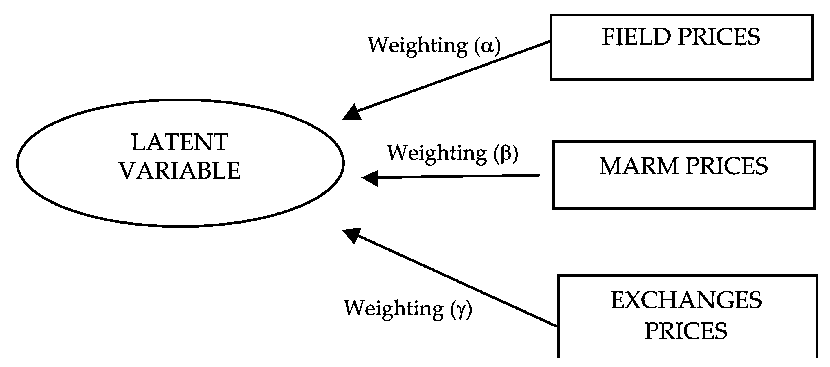
Our factor analysis sought to determine the underlying relationship between three series of data (FIELD prices, MARM prices, and prices in EXCHANGES) in order to establish a criterion for determining the weightings of each of the three sources used (coefficients α, β, and γ in Equation (2)). The model can be represented in a diagram as shown in Figure 2, where the rectangles signify the observed data (each of the three sources used in Equation (2)) and the oval stands for the unobserved data (latent variable). In short, it involved making a regression adjustment where the results obtained were expressed as a percentage in order to be able to make comparisons. AMOS software from SPSS was used.

The main problem for citrus fruit price data when using the above methodology was the non-independence of observations since the value of a datum in one week influenced the value for the following period. Thus, if the quotations (prices) of a variety in one week were 0.23 euro/kilo, the following datum was highly unlikely to have a value of 0.98 euro/kilo since it would be in the vicinity of its predecessor.

However, there was also a second problem due to the fact that the information available was extremely fragmented. In order to be able to use a weekly datum in the analysis, the three values from the three sources of information had to be present in the same week. Since in the case of the Exchange, there are only data from the last two years, the initial series that could be used in this price estimation analysis was restricted to that time period.

Finally, there were a total of 302 useful pieces of data for oranges and 180 useful pieces of data for mandarins out of all the data available. Each of these data thus indicated the value of the quotation for a season, a variety, and a date; hence, their individual analysis led to multiple weighting indexes for each variety depending on the season or period considered. To avoid this, global analyses were carried out for the various varieties on the assumption that all the data for the variety constitute a sample of the quotations for that variety in the seasons available. The results obtained for the data samples of oranges, mandarins, and joint sample (oranges and mandarins) are shown in

Table 5. Results for the aggregation of the varieties of oranges, mandarins, and joint samples.

	Number of Data	MARM	Exchange	Regional Ministries	Sum	RMSA (99% IC)
Oranges; All Varieties	302	0.245 (R2 = 0.910)	0.244 (R2 = 0.911)	0.422 (R2 = 0.952)	0.911	1.174
Mandarines; All Varieties	180	0.076 (R2 = 0.770)	0.150 (R2 = 0.870)	0.620 (R2 = 0.970)	0.846	1.174
Oranges + Mandarins; All Varieties	482	0.153 (R2 = 0.863)	0.228 (R2 = 0.909)	0.509 (R2 = 0.960)	0.890

.

The results derived for the oranges sample show a weighting of 42.2% for Regional Ministry prices and 25% for MARM and Exchanges. This is a good fit for each of the variables considered (the sources of information) since the values of the R² coefficients are very close to one. However, its overall quality is poor, as the RMSA index (the root mean square error approximation index is an estimator of the discrepancies of the data in the population corrected by the degrees of freedom and is the most frequently used global goodness of fit estimator) is always well above 0.08, which is considered to be the highest acceptable value. This poor quality is what means that the sum of the weights for the three variables is not always one. The paucity of data available for the individual variety groups makes it advisable to perform the analysis only on an aggregate basis (oranges, mandarins, and a joint sample of oranges and mandarins), as it is recommended that there be at least 50 observations in order to be able to assume the normality hypothesis in the data.

The results obtained with the aggregated data for mandarins show once again the relevance of Regional Ministry prices with a weight of 62%, a 15% weighting for the Exchanges, and 8% for the MARM. As was the case in the analysis of oranges, the partial fits are good, but as the RMSA index is higher than 0.08, it must be held that the global model lacks the requisite quality, which is why the sum of the weights for the three sources of information is not always one.

The analysis performed with all the data on oranges and mandarins (joint sample), for which 482 useful data are available, reveals once again the relevance of the Regional Ministries as a source of price data with a 51% weight followed by the Exchange prices weighted at 26% and finally the MARM with a weight of 18%.

In order to examine the impact of the data on the results, an analysis was conducted for the Clemenules variety (mandarin) comparing the results of the 74 available pieces of data with the ones in the first 27 of the series (

Table 6. Impact of the data on the results of the SEM weightings.

	Number of Data	MARM	Exchange	Regional Ministries	Sum
Clemenules	74	0.150	0.310	0.540	1
	27	0.230	0.440	0.370	1.04
Navelina	96	0.270	0.220	0.460	0.95
	50	0.130	0.112	0.738	0.98

). In the former case, the Regional Ministries obtained a weighting of 54% and the Exchanges 31%, while in the latter case the Exchanges had a weighting of around 44% and the Regional Ministries’ relative weight fell to 37%. Consequently, we believe that the results of the weightings of the three sources are very sensitive to the data used.

When this analysis was performed again for the Navelina data (orange) by comparing the weights resulting from considering all the available data and some of them, for example the first 50, the results repeated the previous pattern (Table 6). Thus, the weightings found were substantially different from the initial ones in that the relative weight of the Regional Ministries increased from 0.46 to 0.74 with the importance of the other two information sources at around 12%. The above two results thus indicate great sensitivity of the possible weightings to the quality of the data used.

Accordingly, and given the enormous dispersion found for the possible weightings of the sources used both between varieties and within the same variety depending on the data employed, it was decided to add another methodology to the above analysis via a consultation of experts to determine the weightings they attributed to each of the three sources of information being employed (coefficients α, β, and γ).

3.1.2. The Analytic Hierarchy Process (AHP)

Given the above results featuring poor overall quality models, multi-criteria tools were used involving subjective techniques of consultation with experts. In cases where the information is unreliable, insufficient, or simply does not exist, the use of subjective information constitutes an important advance in scientific knowledge. Qualitative methodologies could be a highly efficient resource for obtaining the information necessary for a quantitative economic model. This information proceeds from the knowledge and experience that tacitly resides in the judgement of individual experts. The analytic hierarchy process (AHP) [33] is a decision-making method using pairwise comparisons and relies on the judgement of experts to derive priority scales or preferences. It is these scales that measure intangibles in relative terms. The comparisons are made using a scale of absolute judgements, and this scale represents how much more one element dominates another with respect to a given attribute. It is currently one of the most widely used methods for making choices between alternatives and consists of comparing each one in pairs, indicating preferences on a verbal scale. In short, the AHP provides a reference framework to structure a decision problem, represent and quantify its elements, relate these elements to general objectives, and evaluate alternative solutions.

Saaty [34] argued that, to make a decision in an organized way and generate priorities, we need to decompose the decision into the following steps:

• Define the problem and determine the kind of knowledge sought.
• Structure the hierarchy map. At the top of this map is the decision problem or general objective, at the intermediate level the criteria, and at the lowest level the decision alternatives or options.
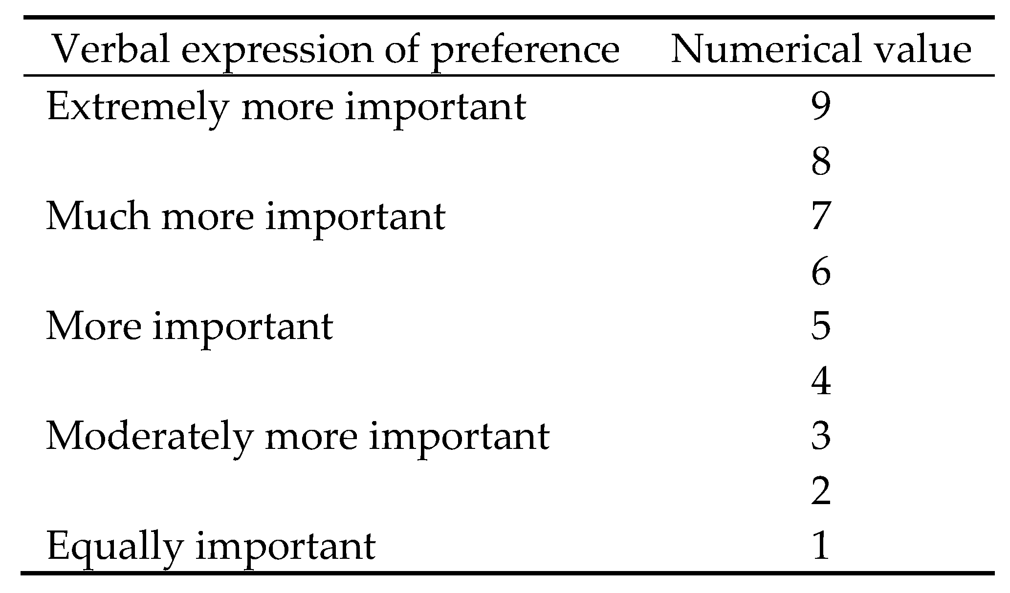
• Construct the pairwise comparison matrix. In this matrix, each element in an upper level is used to compare the elements in the level immediately below it. The elements in each level are evaluated by means of pairwise comparison using a measurement scale from 1 to 9 as shown in Figure 3, which also indicates the numerical correspondence of the verbally expressed preference.

The outcome of these comparisons is a square, reciprocal, and positive matrix called a pairwise comparison matrix, in which each component reflects the intensity of preferences compared to other aspects of the objective under consideration, i.e., the priorities between the different elements compared. In our case, the three elements considered were the three sources of price information (Regional Ministries, MARM, and Exchanges), and the aim was to quantify their level of importance on a scale of 100 points. Therefore, the matrix [3 × 3] reflects the preferences that the experts expressed using the Saaty scale. This matrix has two special features. Firstly, it has ones on the main diagonal because an element must be equally preferred to itself. Secondly, the elements of this matrix meet the condition that aij = 1/aji. In practice, and given the scale used to construct the expert pairwise preference matrix, it is only useful to learn which preference values are greater than one, since the symmetrical value in the matrix will be subtracted from this first value.

The relative weight is then calculated for each element. To do this, each column is added up, and the reciprocal of the total is obtained.

4.

Build the standardized matrix and calculate the priority vector. To do this, an auxiliary matrix is produced in which each cell is completed with the result of the total reciprocal for the value judgement. Adding each row gives the standardized total for each element. The main priorities vector is then derived from the average of the values of the standardized columns. Finally, the result is synthesized from the relative contribution of each alternative to each criterion and the relative level of preference is attributed to them in order to reach the decision problem or general goal.

The research process begins by asking the experts consulted to express their preference for one of the options for each pair analyzed and then asking them to evaluate this importance on the verbal scale shown (Figure 3), which will eventually become numerical. In this specific case, the results obtained derived from consultation with five experts or specialists in the field: three professionals from the citrus fruit industry, one from academia, and another from government.

When methodologies involving several experts are used to determine priorities among various alternatives, as is the case here, there are two possibilities for accomplishing this. The first is to use a single matrix developed as a result of consensus among the experts. The second is to work out the Saaty matrix and the weights associated with it for each of them to finally derive a single solution from the previous values of the individual weights and which usually consists of using the arithmetic mean or the geometric mean of the values of the weights obtained for each decision-maker. Saaty recommends the geometric mean, which tends to attenuate the extreme values of the weights obtained for different experts. However, in this case, the former option was chosen.

The procedure described yielded the results shown in

Table 7. Weighting of the information sources by the experts.

Pairwise Comparison	Most Important Criterion	How Much More (Verbally)	Numerical Value
Regional Minis.—MARM	Regional Minis.	A little more	2
MARM—Exchanges	MARM	Much more important	7
Exchanges—Regional Minis.	Regional Minis.	Extremely more important	9

, derived from the consensus reached among the experts.

The above results were then arranged in the pairwise comparison matrix shown in

Table 8. Pairwise comparisons matrix.

	Regional Ministries	MARM	Exchanges
Regional Ministries	1.00	2.00	9.00
MARM	0.50	1.00	7.00
Exchanges	0.11	0.14	1.00

, bearing in mind that the criterion chosen as most important was the row of the matrix.

The calculations to determine the weights or relative importance of each criterion are as follows. First, the columns of Saaty’s matrix are added up. A new [3 × 3] matrix is then built where each element is the initial one divided by the sum of its column. Finally, the mean value of each of the rows in this new matrix is the weight of the source. The results are shown in

Table 9. Calculation of the weighting of each source of information.

	Regional Ministries	MARM	Exchanges
Column sum	1.611	3.143	17.00
	New matrix			Row sum	Mean weights
Regional Ministries	0.621	0.636	0.529	1.519	0.595
MARM	0.310	0.318	0.412	1.221	0.347
Exchanges	0.069	0.045	0.059	0.260	0.058

.

As noted above, the calculation method originally proposed by Saaty consists of calculating the eigenvector of the pairwise comparison matrix and the eigenvalues associated with it. Given the particular structure of this matrix, there is only one eigenvector in the field of the real ones that corresponded to the weights or relative importance of the compared elements. The method used here was a simplification of the previous one, and its results matched the ones in the method proposed by Saaty when the CR (consistency ratio) value was not very large [35].

In this case, the weighting of the three sources of information based on the preferences expressed by the experts consulted was as follows: 59.5% for information from the Regional Ministries, 34.7% for information from the MARM, and 5.8% for information from the Exchanges. This result may be a good basis for setting the weighting criteria of the different sources.

One aspect often examined in these preferences is the CR of expert estimates. In this case, the CR is 0.02, which is lower than the acceptable value of 0.10. Therefore, these comparisons were admitted as consistent and the simplified calculation method as being appropriate to the data. If the matrix does not achieve the appropriate CR, the initial data must be re-estimated until it is reached.

The above values are similar to and consistent with those found previously. Specifically, they are similar to the results for the mandarin data, where information from the Regional Ministries had a 62% weighting, and to the results for all useful data pertaining to both oranges and mandarins, where the Regional Ministries had a weight of 51%. In the case of the data for oranges, the weight assigned to the Regional Ministries stood at 43%, differing significantly from the figure now derived.

In addition, the values of the weights were calculated exactly following the method advocated by Saaty [33]. In this case, the matrix used had a single solution for the eigenvalue in the real field (the other two solutions were in the imaginary field) and therefore a single eigenvector in the real field, whose values are [0.8623, 0.4996, 0.0827]. Thus, reconverting the previous values so that they added up to one, the values of the weightings were derived by means of the exact method and turned out to be (for Regional Ministries, MARM, and Exchanges, respectively) 0.5969, 0.3458, and 0.0573. Rounding off these values shows that the weight for the Regional Ministries would be 0.60, the weight for the MARM would be 0.35, and the weight for the Exchanges would be 0.05. These results are practically the same as those achieved previously using the approximate method.

Finally, it should be noted that, when the experts were subsequently asked for their opinion on the results previously obtained, they all agreed that they were consistent. When asked why, they mentioned two aspects: firstly, the importance of the Regional Ministries, which are in fact four independent sources and the basis of the MARM calculations; secondly, the low relative importance of the Price Exchanges as a source of information due to the fact that this source of prices has only recently been set up.

In short and according to the previous results, the weighting coefficient values of the sources of information used (coefficients α, β, and γ) for all varieties are as shown in

Table 10. Weighting coefficients of the information sources.

Coefficient	Value
α	0.60
β	0.35
γ	0.05

.

3.2. Weighting Coefficients of Producer Areas (a, b, c, and d)

The weighting coefficients of the field prices of the Regional Ministries for each of the main producer areas in Spain (coefficients a, b, c, and d) were calculated from the average output volumes of each area by variety in the last three years under study (from 2006/2007 to 2008/2009).

The relative weight of each area in the national production of the respective variety was obtained from these output volumes. This relative weight was used to weight the field prices of each variety in each of the four producer areas. The results are shown in

Table 11. Weighting coefficients of producer areas. SOURCE: compiled by the authors on the basis of information from the Regional Ministries and Intercitrus.

MANDARINS	Valencia	Andalusia	Murcia	Catalonia
Satsuma	93%	6%	1%	0%
Clementine	80%	9%	3%	8%
Hybrids	77%	18%	3%	1%
ORANGES
Navelina-Newhall	66%	27%	5%	2%
W. and T. Navel	48%	44%	7%	1%
Navelate/Lanelate	59%	32%	8%	2%
Salustiana	36%	63%	1%	0%
Other white	0%	100%	0%	0%
Blood	63%	35%	2%	0%
Berna	1%	93%	6%	0%
Valencia Late	52%	38%	8%	1%
Other late oranges	0%	100%	0%	0%
LEMONS
Fino	25%	17%	58%	0%
Verna	35%	35%	30%	0%
Other	0%	68%	0%	32%

.

3.3. Weighting Coefficients of Exchange Prices (e and f)

As in the previous case, the weighting coefficients of the prices of the two Exchanges (Valencian Region and Catalonia) (coefficients e and f) were calculated from the average of the output volumes of each area (Valencian Region and Catalonia) by variety in the last three years under study.

The relative weight of each of the two areas (the Valencian Region and Catalonia) in relation to their total output was calculated from these output volumes. This relative weight was used to weight the prices of each variety in each of the two Exchanges. For example: the coefficient of the Valencia Exchange (e) for variety j was

e_j = (Output_j Valencian Region)/(Output_j Valencian Region + Output_j Catalonia).

(3)

The computer application developed calculated the average price for the season from Equation (2), replacing the values of the coefficients previously determined and the weighted season prices of each of the variables involved in determining the APS. The application of this expression to the price series of each variety in a season resulted in the average price for the season of the variety for that season.

3.4. Comparative Analysis of Average Prices for the Season with Field Prices

The methodology described above enabled us to calculate the APS for the 10 seasons under study by variety (grouping of varieties) of orange, mandarin, lemon, and grapefruit. A comparative analysis of the APS of each variety and the corresponding field price in the producer areas for the same variety and season was conducted to obtain an approximate reference for the fit between the calculated APS and the actual citrus fruit prices. In short, it is a question of comparing the result of the econometric formula (Equation (2)) with the values of the variables used in its calculation.

The most representative varieties of Spanish citrus fruit-growing by output volume were analyzed graphically and statistically. The graphs showing the evolution of the average price for the season in the series of seasons studied together with the evolution of the field prices in each area or source of information for the most representative Spanish citrus fruit output varieties were produced using the computer application developed. In addition, graphs were built comparing the APS with all the sources of information in the producer areas (Regional Ministries, MARM, and Exchanges).

Meanwhile, the statistical analysis calculated the average annual deviation (%) between the APS of a variety and season and the corresponding price in the sources of information making up the econometric formula for calculating it (P_VAL, P_AND, P_MUR, P_CAT, MARM, EXCHAN_V, and EXCHAN_CAT). The study covers the 10 seasons surveyed from 2000 to 2009. The analysis differentiated between positive and negative deviations for each of these seasons. A deviation was positive when the average price for the season was higher than the price of the variety considered in that year and in that source of information (Region, Exchange, or MARM).

As noted above, this analysis focused on the main citrus fruit varieties. Thus, in the case of lemons, the cultivars studied were Fino and Verna; for mandarins, the cultivars studied were Clementines and Hybrids; in the case of the oranges, four cultivars were studied: Navelina, Navelate/Lanelate, Valencia Late, and Washington Navel. The deviations from the average price for the season for grapefruit were not examined due to the current paucity of their price data.

The results for the positive and negative average absolute deviations are shown below (

Table 12. Deviations from the average price for the season (lemons, mandarins, and oranges).

Average Absolute Deviations			+ Dev.	− Dev.
LEMONS
	FINO		Average %	Average %
		VALENCIA	0	−11
		MURCIA	3	−2
		ANDALUSIA	n.a.	n.a.
		CATALONIA	n.a.	n.a.
		MARM	6.9	−0.5
	VERNA
		VALENCIA	3.4	3.2
		MURCIA	2.7	−6.3
		ANDALUSIA	n.a.	n.a.
		CATALONIA	n.a.	n.a.
		MARM	4.4	−2.02
MANDARINS			Average %	Average %
	CLEMENTINE
Marisol, Oronules and Clemenules		VALENCIA	10.3	−1.6
		MURCIA	5.5	−7.9
		ANDALUSIA	1.6	−13.6
		CATALONIA	n.a.	n.a.
		MARM	3.9	−15.4
	HYBRIDS		Average %	Average %
Clemenvilla, Fortune and Ortanique		VALENCIA	0.4	−3
		MURCIA	11	−2.7
		ANDALUSIA	13.1	−2.5
		CATALONIA	2.9	−2.62
		MARM	1.34	−1
ORANGES			Average %	Average %
	NAVELINA
		VALENCIA	0	−2
		MURCIA	2	−15
		ANDALUSIA	7	0
		CATALONIA	10	−8
		MARM	2	−1
			Average %	Average %
NAVELATE/LANELATE
		VALENCIA	4	−0.4
		MURCIA	6	−2.9
		ANDALUSIA	0.9	−2.8
		CATALONIA	10	0
		MARM	1	−3.9
			Average %	Average %
	VALENCIA LATE
		VALENCIA	2	−2.3
		MURCIA	7.4	−4.8
		ANDALUSIA	2.5	−4
		CATALONIA	0.4	−8.7
		MARM	3.2	−0.7
			Average %	Average %
	WASHINGTON NAVEL
		VALENCIA	0.06	−6.7
		MURCIA	11.6	−1.5
		ANDALUSIA	3.4	−7
		CATALONIA	13.3	−4.8
		MARM	9.5	−0.4

).

Analysis of the data presented shows that the deviations in the last 10 seasons considered between the average price for the season and the price of the variety in that Region rarely exceeded 10% (above or below the average price for the season) for the eight varieties of citrus fruit analyzed. Specifically, only five cases were detected out of the 70 analyzed, and this was usually because the data in the season or in the respective producer area were unrepresentative. It is therefore not unreasonable to conclude that, on the whole, the calculated average price for the season fairly accurately represents the mean price of the variety in the region. Accordingly, if this continues to be the case, then the calculated average price for the season will accurately represent the prices of each variety in each region.

4. Conclusions

The formula for calculating the average price for the season (APS) (in €/kg) has been defined mathematically based on the selected variables weighted by coefficients that represent the relative weight of the various sources of price information and producer areas. The results of the analysis comparing the APS with the corresponding quotations from the sources of information used to formulate it show that for the main citrus fruit varieties in the 2000–2009 historical series, the deviations between the APS and the price of the variety in each producer area did not generally exceed ±10%. When they did, it was usually because the data in the season or in the respective producer area were unrepresentative. This ensures the APS’s fit with the actual field quotations in the country’s producer areas. This methodological application constitutes the principal scientific contribution of the investigation. Its current relevance and validity resides in the fact that the method permits a methodological proposal to be generalized for use in other studies of similar characteristics in the field of agricultural insurance.

It can therefore be concluded that, on the whole, the APS represents the mean price of the variety in the producer areas fairly accurately. It is a price subject to the laws of a market that is not controllable [36] and behaves randomly because it is derived from actual information generated by the fresh citrus fruit markets judged to be the most representative. It is an index and consists of a weighted combination of market prices and quotations, which makes it possible to establish and explain citrus fruit field prices. It is set for a given geographical area and variety or group of crop varieties with similar market behavior. The idea is that the producer should perceive that the price to be used to assess potential revenue insurance compensation is as representative as possible of the price at which they actually sell their crop. The formula for calculating APS does not include data in period (t − 1) because the price for the season t is independent of that for the season (t − 1), since the t value is only influenced by current market situation. The insurance is indexed, which means that when the conditions for triggering the revenue cover are met, all farmers who are insured in the geographical area or for the relevant variety or varieties will be compensated.

Sources of citrus fruit price information should be public, accessible, and updatable without undue delay. For these purposes, the following are initially considered: The Price Observatory of the Regional Ministry of Agriculture, Fisheries and Food of the Valencian Regional Government; the Price and Market Observatory of the Andalusian Regional Government; the Food Price Observatory of the Ministry of the Environment, Rural and Marine Affairs; and the field Exchanges.

A historical APS series has been drawn up using the historical information available, which is sufficiently comprehensive to be used in revenue risk calculation studies. In addition, market prices will have to be monitored for the insurance coverage so as to provide information during the season on the APS’s evolution over time and the mean price of the whole.

Regarding the time component, the reference price can be calculated on the basis of the historical series of the APS for the number of seasons and the criteria to be determined. It will be the insured price at which the revenue insurance is deemed to be triggered. A percentage of the mean value of the APS for a given number of seasons or a lower price, which nonetheless compensates basic production costs, may be used to determine the reference price. In all cases, and given that the purpose of the insurance is to cover short-term and very sharp price falls in specific seasons, the deviation of the APS from the reference price has to be significant.

The configuration of revenue insurance should be in line with the World Trade Organization’s Marrakesh Agreement on Agriculture as well as the criteria identified by the European Commission in its Communication to the Council on risk and crisis management in agriculture (2005). Compliance with both requirements makes it possible for the government to participate financially in Income Insurance and Income Safety Net programmes. The following conditions have to be met to be eligible for these payments:

• loss of income (considering only income derived from agriculture) must be greater than 30% of average gross income or its equivalent in net income (excluding any other payments received from the same or similar schemes);
• the amount of the payments will compensate for less than 70% of the producer’s loss of income in the year in which the producer is eligible for such assistance;
• the amount of any such payment will relate solely to income;
• when a producer receives payments under this heading and relief in case of natural disasters in the same year, the total of such payments will be less than 100% of the producer’s total loss.

The producer should take out crop yield insurance to cover catastrophic damage as well as additional coverage against catastrophic price shocks (with losses of more than 30%). If only production damage is sustained on the farm, the insured producer would be compensated under the terms of the relevant crop yield insurance contract.

Agriculture is a strategic sector of the economy due to its ties to elements essential to the quality of life of a country’s population: i.e., food supplies and the environment. At the same time, agriculture makes use of natural resources that impose costs on economies and make agricultural systems less efficient. Agriculture should be a leader in change towards sustainable growth by promoting innovative technologies and production systems. That is the reason why sustainable growth of the agricultural sector is a necessity from the perspective of the environment, society, and the economy. The term “sustainable agriculture” calls for management of natural resources in a way that ensures that their benefits are also available for the future, and is one of the priorities of the EU’s development cooperation. One of the objectives of the EU’s sustainable agriculture and rural development policy is strengthening agricultural markets by reducing the exposure of agricultural producers to market risks, like price volatility.

Finally, without invalidating the conclusions drawn from the results given their high level of reliability and validity, we note the following limitations to the study to be taken into consideration in future research:

−

The price series used were taken from previous citrus fruit growing seasons that differ in time from the current one. This is due to the need to have price series that were as comprehensive as possible, the time required in some of the sources consulted to make public the prices of completed seasons, and, in particular, the time the research team needed to conclude all the stages of the study (much more wide-ranging than what is strictly included in this paper). Nevertheless, as this paper’s main contribution is the methodological proposal for the determination of the APS, we consider that this limitation does not invalidate the results and that our conclusions can be obtained.

−

The inclusion in the average price for the season of the prices of the Ministry of Agriculture (MARM) means they must be published, given that the average price for the season is public and can be replicated. The MARM price information used in this study was provided by the State Agency for Agricultural Insurance (ENESA), although it is not at present publicly accessible.

−

The existence of marketed varieties for which price information is not published in the various sources of field prices means that groups of varieties need to be set up in order to calculate the average price for the season and the reference price. As a result, all the varieties in the same grouping will have the same average price for the season.

References

1. Iyer, P.; Bozzola, M.; Hirsch, S.; Meraner, M.; Finger, R. Measuring Farmer Risk Preferences in Europe: A Systematic Review. J. Agric. Econ. 2019. [Google Scholar] [CrossRef] [Green Version]
2. OECD. Income Risk Management in Agriculture; Organization for Economic Cooperation and Development: Paris, France, 2000; 151p. [Google Scholar]
3. OECD. Risk Management in Agriculture. A Holistic Conceptual Framework; Working Party on Agricultural Policies and Markets: Paris, France, March 2009. [Google Scholar]
4. El Benni, N.; Finger, R.; Meuwissen, M.P. Potential effects of the income stabilisation tool (IST) in Swiss agriculture. Eur. Rev. Agric. Econ. 2016, 43, 475–502. [Google Scholar] [CrossRef]
5. Meuwissen, M.P.; Mey, Y.D.; van Asseldonk, M. Prospects for agricultural insurance in Europe. Agric. Financ. Rev. 2018, 78, 174–182. [Google Scholar] [CrossRef]
6. Cordier, J. Comparative Analysis of Risk Management Tools Supported by the 2014 Farm Bill and the CAP 2014–2020; European Parliament, Directorate-General for Internal Policies, European Union: Brussels, Belgium, 2015. [Google Scholar]
7. Pennings, J.M.; García, P. Hedging behavior in small and medium-sized enterprises: The role of unobserved heterogeneity. J. Bank Financ. 2004, 28, 951–978. [Google Scholar] [CrossRef]
8. Pennings, J.M.; Wansink, B. Channel contract behavior: The role of risk attitudes, risk perceptions, and channel members’ market structures. J. Bus. 2004, 77, 697–724. [Google Scholar] [CrossRef] [Green Version]
9. Turvey, C.G. Whole Farm Income Insurance. J. Risk Insur. 2012, 79, 515–540. [Google Scholar] [CrossRef]
10. Just, D.R.; Just, R.E. Empirical identification of behavioural choice models under risk. Am. J. Agric. Econ. 2016, 98, 1181–1194. [Google Scholar] [CrossRef]
11. Thompson, S.R.; Schmitz, P.M.; Iwai, N.; Goodwin, B.K. The real rate of protection: The income and insurance effects of agricultural policy. Appl. Econ. 2004, 36, 1851–1858. [Google Scholar] [CrossRef]
12. Walters, C.; Preston, R. Net income risk, crop insurance and hedging. Agric. Financ. Rev. 2018, 78, 135–151. [Google Scholar] [CrossRef]
13. Janowicz-Lomott, M.; Lyskawa, K.; Rozumek, P. Farm income insurance as an alternative for traditional crop insurance. Procedia Econ. Financ. 2015, 33, 439–449. [Google Scholar] [CrossRef] [Green Version]
14. European Commission. EU Farm Economics Overview; Directorate-General for Agriculture and Rural Development: Brussels, Belgium, 2018; Available online: https://ec.europa.eu/info/sites/info/files/food-farming-fisheries/farming/documents/eu-farm-economics-overview-2015_en.pdf (accessed on 8 September 2019).
15. Williams, J.R.; Saffert, A.; Barnaby, G.A.; Langemeier, M.R. The impact of whole-farm gross revenue insurance on farm income variability. J. Agric. Resour. Econ. 2007, 32, 563. [Google Scholar]
16. Garrido, A.; Bardají, I. Strategies for the management of risks and crises in Spanish agriculture. Revista Española de Estudios Agrosociales y Pesqueros 2009, 221, 175–205. [Google Scholar]
17. Meuwissen, M.P.; Huirne, R. Feasibility of income insurance in European agriculture. Am. J. Agric. Econ. 1998, 80, 1171. [Google Scholar]
18. Meuwissen, M.P.; Huirne, R.B.M.; Hardaker, J.B. Income Insurance in European Agriculture; European Economy, Reports and Studies No. 2; Office for Official Publications of the European Communities: Luxemburg, 1999. [Google Scholar]
19. Caffeiro, C.; Capitano, F.; Cioffi, A.; Coppola, A. Risk and Crisis Management in Agriculture; European Parliament Document; European Parliament: Brussels, Belgium, 2005; IP/B/GRI/ST/205-3. [Google Scholar]
20. European Commission. Agricultural Insurance Schemes; DG Agriculture and DG Joint Research Centre: Brussels, Belgium, 2006; Available online: https://ec.europa.eu/agriculture/sites/agriculture/files/external-studies/2006/insurance/full-report_en.pdf (accessed on 10 September 2019).
21. Mateos-Ronco, A.; Server, R.J. Drawing up the official adjustment rules for damage assessment in agricultural insurance: Results of a Delphi survey for fruit crops in Spain. Technol. Forecast. Soc. Chang. 2011, 78, 1542–1556. [Google Scholar] [CrossRef]
22. Enjolras, G.; Capitanio, F.; Aubert, M.; Adinolfi, F. Direct payments, crop insurance and the volatility of farm income. Some evidence in France and in Italy. In Proceedings of the 123rd EAAE Seminar “Price Volatility and Farm Income Stabilisation”, Dublin, Ireland, 23–24 February 2012. [Google Scholar]
23. Burgaz, F.J. ‘Pasado y presente de los seguros agrarios: Lecciones aprendidas y futuros desarrollos’. In International Conference “El seguro agrario como instrumento para la gestión de riesgos”; ENESA (MAPA): Madrid, Spain, 2006. [Google Scholar]
24. Goodwin, B.K.; Hungerford, A. Copula-based models of systemic risk in US agriculture: Implications for crop insurance and reinsurance contracts. Am. J. Agric. Econ. 2014, 97, 879–896. [Google Scholar] [CrossRef] [Green Version]
25. Mahul, O. Hedging price risk in the presence of crop yield and revenue insurance. Eur. Rev. Agric. Econ. 2003, 30, 217–239. [Google Scholar] [CrossRef]
26. Coble, K.H.; Heifner, R.G.; Zuniga, M. Implications of crop yield and revenue insurance for producer hedging. J. Agric. Resour. Econ. 2000, 25, 432–453. [Google Scholar]
27. Goodwin, B.K.; Roberts, M.C.; Coble, K.H. Measurement of price risk in revenue insurance: Implications of distributional assumptions. J. Agric. Resour. Econ. 2000, 25, 195–214. [Google Scholar]
28. MARM. Anuario de Estadística; Ministerio de Medio Ambiente, Medio Rural y Marino: Madrid, Spain, 2009; Available online: http://www.mapa.es/es/estadistica/pags/anuario (accessed on 15 February 2019).
29. Hair, J.F.; Anderson, R.E.; Tatham, R.L.; Black, W.C. Multivariate Data Analysis, 5th ed.; Prentice-Hall Iberia: Madrid, Spain, 1999. [Google Scholar]
30. Hair, J.F.; Black, W.C.; Babin, B.J.; Anderson, R.E.; Tatham, R.L. Multivariate Data Analysis, 6th ed.; Prentice Hall: Upper Saddle River, NJ, USA, 2006. [Google Scholar]
31. Byrne, B.M. Structural Equation Modeling with AMOS. Basic Concepts, Applications, and Programming, 2nd ed.; Routledge: Abingdon, UK, 2010. [Google Scholar]
32. Blunch, N.J. Introduction to Structural Equation Modelling Using SPSS and AMOS; SAGE: London, UK, 2008. [Google Scholar]
33. Saaty, T.L. Fundamentals of the Analytical Hierarchy Process. In The Analytic Hierarchy Process in Natural resource and Environmental Decision Making; Schmoldt, D.L., Kangas, J., Mendoza, G.A., Pesonen, M., Eds.; Springer: Amsterdam, The Netherlands, 2001; Volume 3, pp. 15–35. [Google Scholar]
34. Saaty, T.L. Decision making with the analytic hierarchy process. Int. J. Serv. Sci. 2008, 1, 83–98. [Google Scholar] [CrossRef] [Green Version]
35. Anderson, D.; Sweeney, D.; Williams, T. Métodos Cuantitativos para los Negocios; Thomson: Madrid, Spain, 2004. [Google Scholar]
36. European Commission. Communication from the Commission to the Council on Risk and Crisis Management in Agriculture; DG Agriculture and Rural Development: Brussels, Belgium, 2005; Available online: https://ec.europa.eu/transparency/regdoc/rep/1/2005/EN/1-2005-74-EN-F1-1.Pdf (accessed on 20 October 2019).
Figure 1. Citrus fruit value chain.
Agronomy 10 00198 g001
Figure 2. SEM model for determining the weighting of sources of information.
Agronomy 10 00198 g002
Figure 3. Verbal scale of preferences.
Agronomy 10 00198 g003