Article

Mechanical Devices for Mass Distribution Adjustment: Are They Really Convenient?

Department of Agricultural and Food Sciences, Alma Mater Studiorum, Università di Bologna, 40127 Bologna, Italy
*
Author to whom correspondence should be addressed.
Agronomy 2020, 10(11), 1820; https://doi.org/10.3390/agronomy10111820
Submission received: 17 October 2020 / Revised: 9 November 2020 / Accepted: 18 November 2020 / Published: 20 November 2020
(This article belongs to the Special Issue Life Cycle Sustainability Assessment of Agricultural Machinery)

Abstract

:
Since the introduction of four-wheel drive (4WD) and especially front wheel assist (FWA), many studies have been conducted on the optimal weight distribution between tractor front and rear axles because this influences traction efficiency. The aim of this paper is to evaluate the traction and efficiency advantages in the adoption of mechanical ballast position adjustment devices. The tested device is an extendable ballast holder mounted on the front three-point hitch of the tractor, able to displace the ballast up to 1 m away from its original position. An estimation of the fuel consumption during ploughing with the extendable ballast holder in different configurations was performed. Tractive performance was evaluated through drawbar tests, performed on loam soil with a 4WD tractor having a maximum engine power of 191 kW and a ballasted mass of 9590 kg. Results show that changing the tractor weight distribution over the range allowed by the extendable ballast holder produces limited effects in terms of tractive performance and fuel saving. The adoption of such devices is thus ineffective if other fundamental factors such as tyre pressure, choice of the front-to-rear wheel combination and lead of the front wheels are not considered during tractor setup.

1. Introduction

The need to minimize operational costs and the growing attention on the environmental impact of human activities have fostered several studies on energy usage in farming in the last decades. Agriculture is not only an energy demanding activity, but it also contributes to about 20% of the global emissions of greenhouse gases, notably methane and nitrous oxide [1]. Moreover, the growth in food demand due to the increase in the world population implies that modern agriculture needs to increase productivity and efficiency at the same time [2]. One of the solutions adopted to reach these goals is the use of more powerful and efficient machines, hence four wheel drive (4WD) and especially front wheel assist (FWA) tractors have gained increasing importance compared to two wheel drive (2WD) tractors in the last decades [3]. However, the potential advantages in terms of efficiency and productivity obtainable with the adoption of a FWA tractor could be undermined by improper ballasting, which can impair traction performance. In fact, the tractor weight distribution between front and rear axles determines the maximum available drawbar pull under a given slip and, in turn, also determines the wheel slip for a given drawbar load [4]. For FWA tractors, previous studies have demonstrated that the maximum traction efficiency on soil or concrete is obtained with a ballast distribution with approximately 40 to 45% of the total static load on the front axle and a front/rear wheel speed ratio from 1.01 to 1.05. Furthermore, tractive efficiency is more sensitive to the dynamic load distribution when the tractor operates on loose soil than when it operates on concrete [5]. The estimation of the correct ballasting is strongly related to many parameters, such as soil conditions [6,7], tire type and inflation pressure [8,9], front and rear wheel radius, lead of the front wheels [10] and field operation [11,12]. Generally, for a given value of slip, the tractive efficiency of a driving wheel increases with an increase in dynamic load on compacted soil, and decreases with an increase in dynamic load on loose soils [13]. The first attempts to predict the correct ballasting for every working condition were mainly empirical [14]. Especially during the 1970s, empirical models were proposed by tractor manufacturers to their customers using simple tables that considered parameters like tractor weight, maximum power, tire size and speed of the field operation [15]. Many analytical models regarding the influence of tractor load distribution on traction efficiency were based on the traction equations developed by Brixius and Wong [16,17]. The results showed that tractive performance is strongly dependent on the gross traction ratio (GTR). GTR is the pull a tractor would develop if there was no motion resistance losses and it is the ratio between the traction force and the dynamic load on the wheel. Tractors do not always operate at constant working conditions, hence an optimum level of ballast that fits every condition is unreachable. A ballast configuration that generates a GTR of 0.54 is considered a good compromise, since it permits good traction performance over a wide range of operational conditions [18].
Even though many studies have focused on the relationship between weight distribution and traction efficiency [19,20,21,22,23,24,25,26], none of these provided an estimation of the fuel saving obtained in optimal operational conditions. In recent years, agricultural machinery manufacturers have invested in the development of devices able to conveniently modify the tractor load. Examples are the EZ-ballast (John Deere, Moline, IL, USA), that reduces the time required to install the ballast on the tractor, and the Grip Assistant (Fendt, Kempten, Germany), a piece of built-in tractor software that suggests to the user the optimal ballast level and automatically adjusts the tire pressure. Another example of these innovative ballast systems is the Multiplier Counterweight (MC) designed by ALI s.r.l. (Anghiari, AR, Italy). This device is a special ballast holder that can be installed either on front or rear three-point hitch and is able to displace the ballast up to 1 m away from its original position in the longitudinal direction. Ballast movement is facilitated by a mechanical linkage actuated by the tractor hydraulic system. The concept of changing tractor load distribution by moving the ballast forward is not completely new [27], but no device of this type has ever reached the market. The aim of this paper is to evaluate the advantages in the adoption of such mechanical ballast position adjustment devices. To this end, a comparative analysis is conducted of the regression curves and the prediction bounds of tractive efficiency and net traction ratio, obtained from field tests involving a tractor with three different front/rear axle weight distributions. In addition, the economic impact that the adoption of a ballast position adjustment devices could have on agricultural activities is estimated by theoretically predicting productivity and fuel consumption during ploughing.

2. Materials and Methods

A tractor ballasted with the MC was tested to compare its tractive performance in different device configurations (Figure 1). Ballast displacement was performed through a mechanical linkage actuated by the tractor hydraulic remotes. The mass of the bare device (i.e., with no ballast connected) was 500 kg and the ballast chosen to perform the tests had a mass of 500 kg; hence, the total mass of the system comprising the MC and the ballast was 1000 kg; that is, the mass of a standard front ballast designed for the tractor used in the tests.
Tests were carried out with a New Holland T7.260 (CNH Industrial N.V., Amsterdam, NL) (TT), equipped with the MC on the front three-point linkage. Tractor specifications are reported in Table 1.
Three different static mass distributions on the tractor axles were tested by changing the tractor ballast configuration (Table 2). In the first configuration, the MC was fully extended (configuration “FE”); in the second, the MC was fully closed (configuration “FC”); for the third configuration, a 1000 kg standard ballast was mounted on the rear three-point linkage of the tractor (configuration “R”).
In order to compare the tractive performance of the TT in FC, FE and R configurations, drawbar tests were carried out towing a Case IH Maxxum 115 (CNH Industrial N.V., Amsterdam, NL, The Netherlands) (LU) properly ballasted. The two tractors were joined using a steel chain and a load cell (NBC Elettronica, Sondrio, Italy) to measure the draught force (FD) during the tests (Figure 2).
The actual speed (v) of the tractor was monitored with a GPS receiver (IPESpeed, IPETronik GmbH, Baden Baden, Germany) and recorded on a CAN-Bus data logger (CanCase XL Log, Vector Informatik, GmbH, Stuttgart, Germany). The data logger was connected to the CAN-Bus network of the tractor, which allowed other parameters such as engine speed (ne), engine torque (Te) and selected gear to be acquired simultaneously, while the engine power (Pe) was calculated using the method reported in Molari et al. [28]. Tests were performed on a loam soil [29] field with a moisture content [30] of 16.87% (dry basis) and plastic limit and liquid limit [31] of 22.6% and 36.2%, respectively. In order to reduce data scattering, drawbar tests were carried out using the constant draught test procedure [32,33] for all the three tested weight distribution configurations. Thus, the TT during the tests was always maintained at full throttle, while the drawbar pull could be varied by manipulating the throttle lever and the engaged gear of the LU. Tests were carried out at 3 different gears of the TT (7th, 8th and 9th) and 5 different travelling speeds were obtained for each gear by changing the drawbar pull applied by the LU. The gear ratios ( τ ) of the tractor rear wheels to the engine crankshaft are reported in Table 3.
Each travelling speed was maintained for a running length of 30 m after its stabilization in order to reach a steady-state condition. Overall, 15 different test conditions were tested; each of these was replicated 3 times to increase the number of samples. The described procedure was adopted for all the considered mass distributions over the TT axles (FC, FE and R).
The average travel reduction ratio (s, commonly called “slip”) of the TT over the running length of 30 m in every test condition was calculated as follows:
s = (NlNul)/Nl,
where Nl and Nul are the number of revolutions performed by the TT engine crankshaft over the 30 m of running length with and without drawbar pull applied by the LU, respectively, and are calculated by integrating ne over the time duration of each test run. The mean values of FD, v and Pe over each of the 30 m runs were also calculated. Moreover, the evaluation of the standard deviation of FD (σFD) and v (σv) over each run were used to verify that tests were performed in almost steady-state conditions. Indeed, samples that achieved values of σFD greater than 500 N or of σv greater than 0.2 km/h were not considered valid. Then, traction efficiency (ηT) and the net traction ratio (NTR) were calculated, respectively, as:
ηT = (FD v)/Pe
NTR = FD/(M g)
where g is the gravitational acceleration.

2.1. Interpolation of Data Obtained from Experiments

A regression analysis was performed on the experimental data to find the variation of ηT as a function of s, of NTR as a function of s and of ηT as a function of NTR for each of the three tractor configurations tested. The regression models used are shown in Table 4.
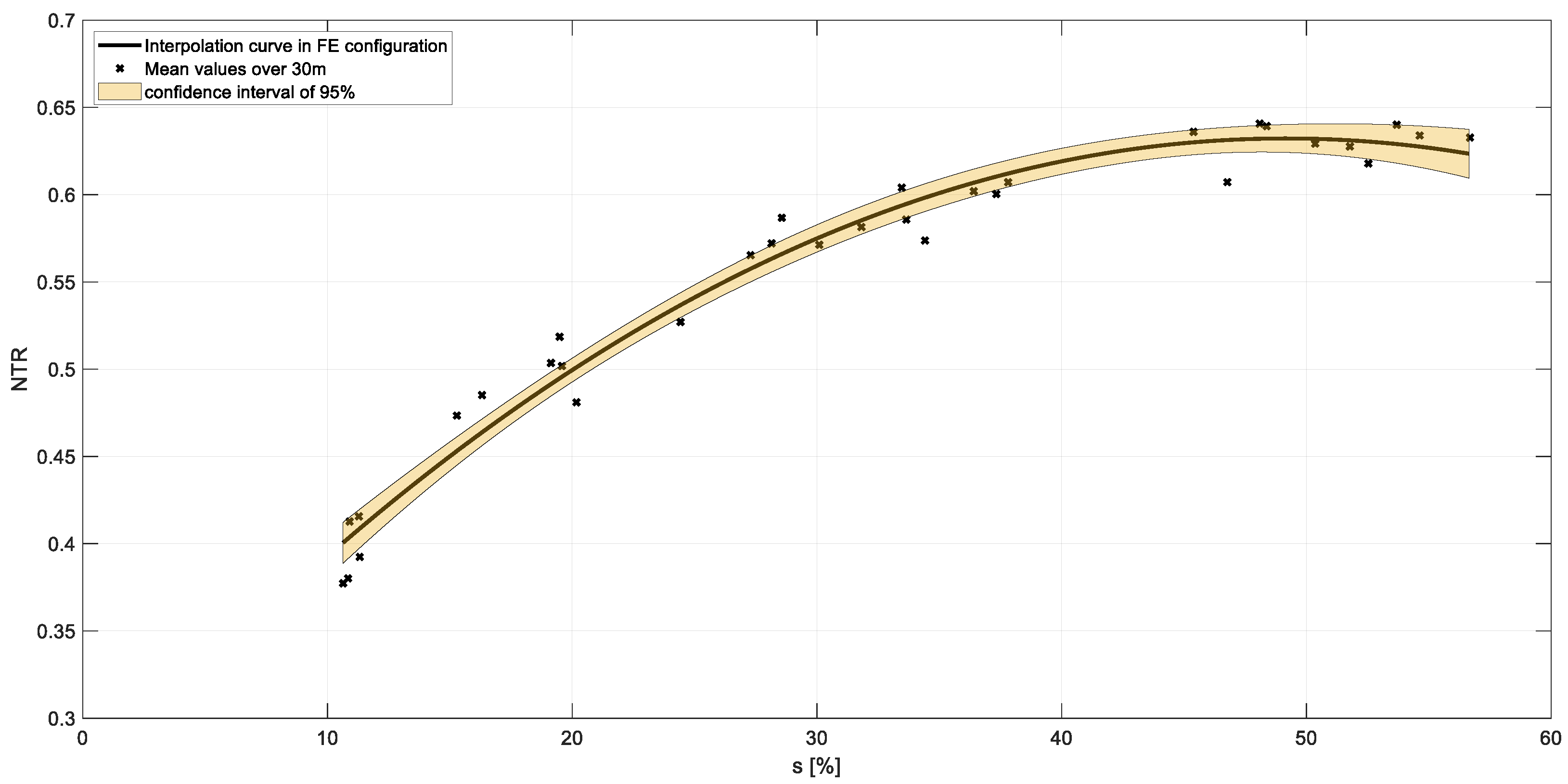
Since the regression curves for the three tractor configurations were close to one another, data analysis and interpretation were conducted upon the evaluation of the upper and lower prediction bounds (95% confidence level) for the regression curves R1, R2 and R3. The algorithm used to find these confidence bounds was the MATLAB function predint (MATLAB®, Mathworks, Inc., Natick, MA, USA). For each regression model, the same upper and lower bounds of the independent variable were chosen for the three tractor configurations, and, for each regression curve, the area enclosed between the upper and the lower prediction bounds was determined (Figure 3).
The analysis of the effect of a change in tractor mass distribution was then conducted by comparing the overlap in the prediction bound areas. Indeed, a significant (or full) overlap in the prediction bound area of one of the regression curves with that of another regression curve indicates that the two regression curves are not significantly different [34].

2.2. Field Productivity and Fuel Consumption Prediction

The economic impact that the adoption of devices such as the MC could have on agricultural activities was estimated by predicting productivity and fuel consumption during a typical operation. To this end, a reference field operation was simulated through a procedure that involved the estimation of the net traction ratio exerted by the implement and the determination of the tractor engine working point. Ploughing was chosen as the reference operation. Upon choosing plough dimensions compatible with the TT class, the net traction ratio exerted by the implement (NTRplough) was estimated using the ASAE/ D497.7 standard [35]:
NTRplough = {0.7 × [652 + 5.1 v2] × Wi × Di}/M
where Wi (in meters) is the implement width, set equal to 2.2 m, and Di (in centimeters) is the working depth, set at 35 cm. As for the plough parameters, soil parameters were chosen to simulate a plausible working condition for the TT.
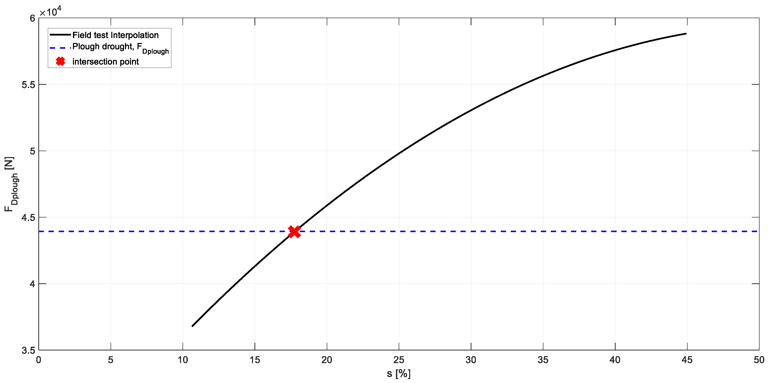
Then, for each MC configuration, the expected working condition of the tractor-plough system (Figure 4) was determined by computing the intersection between the curve described by Equation (4) and the regression curve E1 (Table 5), assuming that the reference operation was carried out with the TT in 8th gear. A preliminary analysis showed no remarkable differences in the results if the tractor was assumed to work either in 7th or 9th gear. The R configuration was not considered since it would not be replicable during ploughing.
After the expected working condition is determined in terms of v and NTR, the working draught force (FDplough) and the power absorbed (Pplough) by the implement are computed as follows:
FDplough = NTR M g
Pplough = FDplough v
While the operation productivity ( Π ) is obtained by:
Π = v Wi. ηf
where ηf is the field efficiency, equal to 0.85, which is the standard value for a moldboard plough [35].
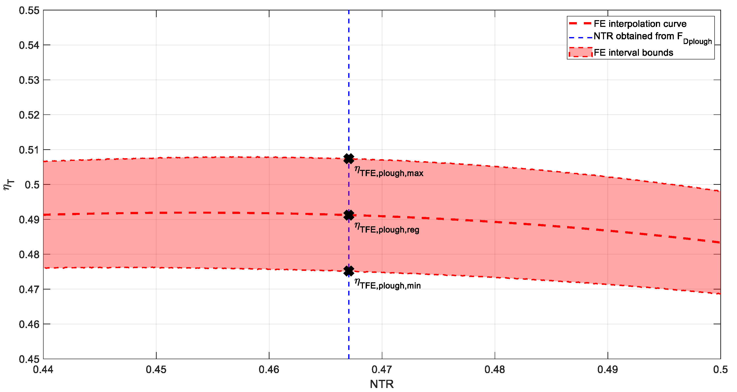
Next, in order to obtain a prediction of the fuel consumption for each tractor during the reference operation, the engine torque and rotational speed were estimated. To this end, traction efficiency was computed through the regression model R3 and also using the upper and lower prediction bounds for each regression model (Figure 5). Therefore, for each tractor configuration, three values of traction efficiency were obtained:
ηT ic,min, ηT ic,reg, ηT ic,max
where ic = FE, FC are the indices for the tractor configuration.
The engine power is then computed as:
Pe = Pplough/ηT
In order to estimate engine rotational speed, the expected value of tractor slip during the reference operation was computed through the regression curve E2 (Table 6) for each tractor configuration, starting from the expected value of FDplough previously determined (Figure 6).
From the expected value of tractor slip and speed, the theoretical tractor speed (vth) is determined:
vth = v/(1 − s)
Then, the engine speed and delivered torque during the reference operation are estimated for each tractor configuration:
ne = [vth/(rr τ)] (60/2π)
Te = (60 Pe)/(2π ne)
To estimate the specific fuel consumption (Cs) of the TT during the reference operation, an empirical equation was developed and validated through tests performed at the PTO test bench located at the Agricultural Mechanics Laboratory of University of Bologna located in Cadriano, Italy:
Cs = 460.1 − 26.28 (ne/nrated) − 606.4 (Te/Tmax) + 72.97 (ne/nrated)2 − 12.11 (ne/nrated) (Te/Tmax)) + 325.4 (Te/Tmax)2
Once Cs is known, the hourly fuel consumption (Ch) and the fuel consumption per hectare (Cha) are obtained as follows:
Ch = (Cs × Pe)/ρ
Cha = Ch/Π
where ρ is the fuel density, equal to 850 kg/m3.

3. Results

3.1. Tractive Performance

The regression parameters and curves of the regression models R1, R2 and R3 are shown in Table 7, Table 8 and Table 9 and in Figure 7, Figure 8 and Figure 9, respectively.
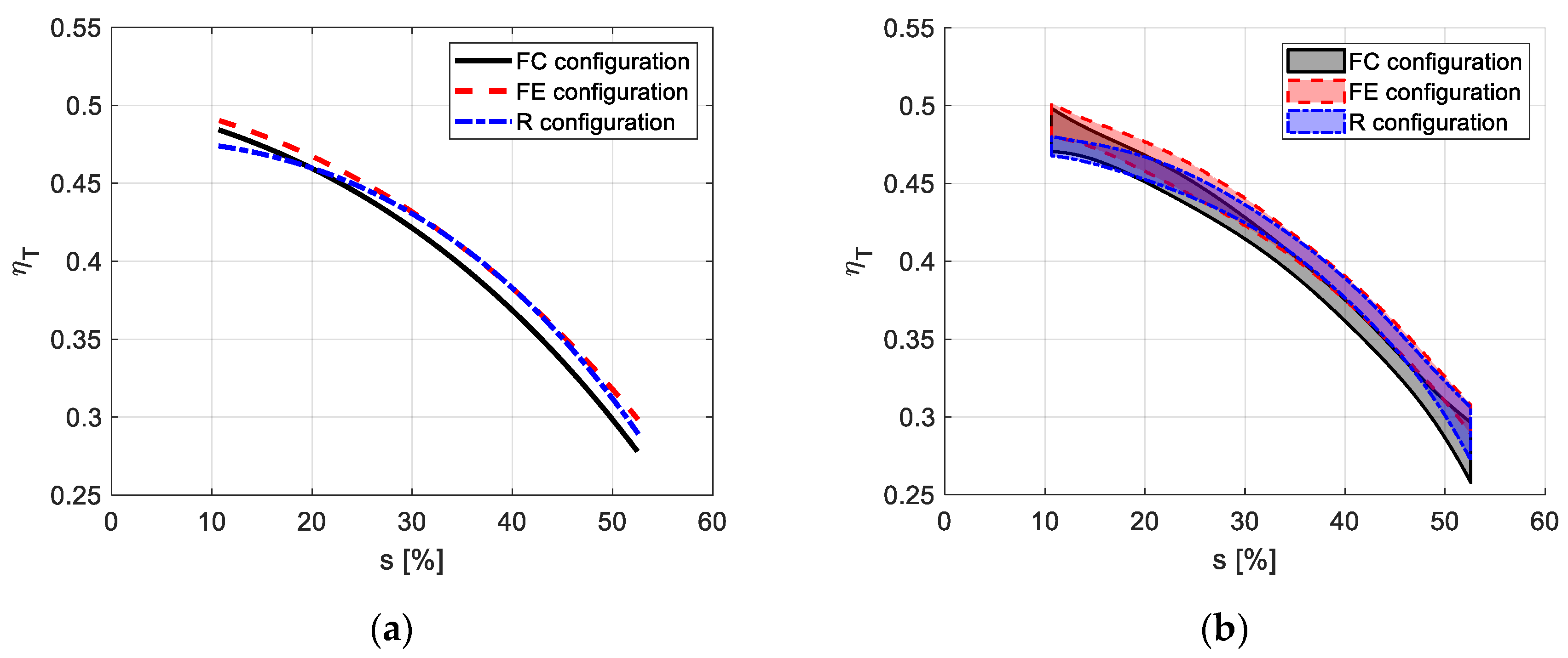
From the regression curves depicted in Figure 7 for the three different tractor configurations, it can be observed that traction efficiency decreases as tractor slip increases; this behavior is consistent with the available literature in the range over 10% tractor slip [36]. Figure 7a also shows that the FE and R regression curves almost entirely overlap, especially for values of tractor slip over 30%. On the other hand, the FC regression curve is shifted towards lower values of ηT with respect to the case of FE. However, the difference between the two curves is very limited, with the maximum difference in ηT for a given value of tractor slip being 0.02. Furthermore, a comparison of the prediction bound areas (Figure 7b) confirms that FE and R regressions deeply overlap: 73% of the R prediction bound area is included in that of FE. The prediction bound area for configuration FC significantly overlaps with that of FE only for values of tractor slip lower than 20%, whereas globally the two areas overlap for the 31% of their extension.
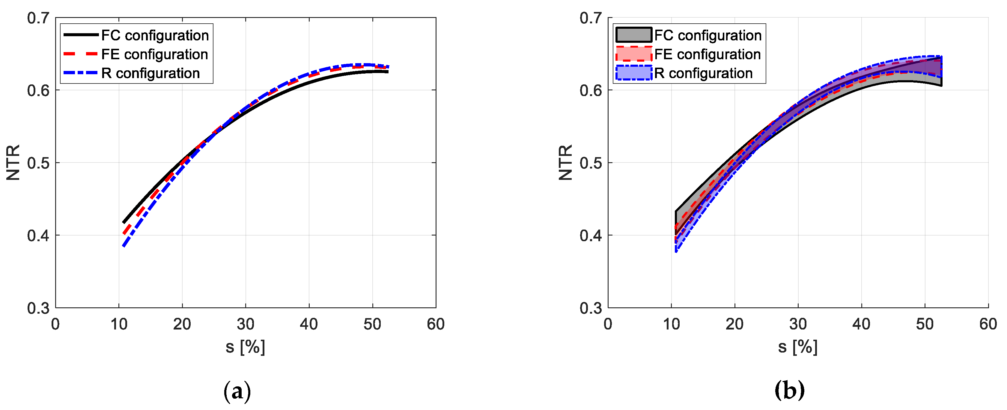
Figure 8a shows that the net traction ratio increases with increasing tractor slip, reaching maximum values at around 40–50% tractor slip; this trend is consistent with the literature [7]. Figure 8 also shows that the regression curves are very close to one another, with minor differences visible only at low and high values of tractor slip. FE and R configurations reach a maximum net traction ratio of 0.64, only 1% higher than FC configuration. The analysis of the prediction bound areas (Figure 8b) confirms that the FC, FE and R regression models are almost identical. In fact, around 70% of the FE prediction bound area is included in that of FC and R. The areas overlapping between the FC and R configurations are less relevant, but 50% of the FC prediction bound area is still included in that of R.
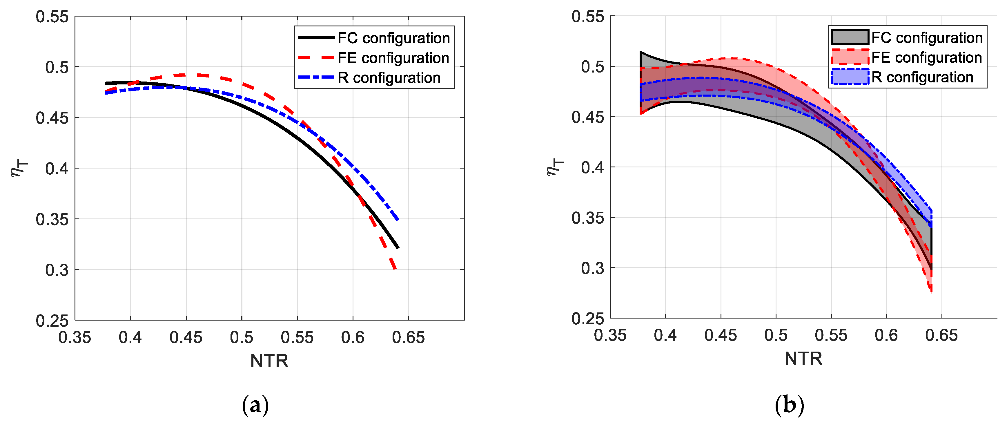
As depicted in Figure 9a, tractive efficiency increases at low values of net traction ratio for all tractor configurations, reaching a peak at values of NTR in the range 0.40–0.45; beyond these values, the trend begins to decrease. This behavior is consistent with the literature [19]. The maximum values of traction efficiency as estimated by the FE, FC and R regression models were 0.49 (at NTR = 0.45), 0.48 (at NTR = 0.40) and 0.48 (at NTR = 0.43), respectively. Results show that the usage of the MC in FE configuration permits an advantage in terms of traction efficiency over the other configurations in the net traction range 0.45–0.55; however, this advantage is scarce. Indeed, the maximum difference in tractive efficiency between FE and FC configurations is only 0.02, registered at NTR = 0.52. The analysis of the prediction bound areas (Figure 9b) shows that the areas are rather wide compared to those obtained for the ηT-s and NTR-s regression models; in particular, the area for the FC configuration is 17 and 56% wider than that for the FE and R configurations, respectively. There is a pronounced overlap between the three prediction bound areas; indeed, 64 and 66% of the R configuration area is included in the FE and FC areas, respectively. FC and FE areas overlap for 50% of their extension.

3.2. Cost-Effectiveness Analysis in FE and FC Configurations

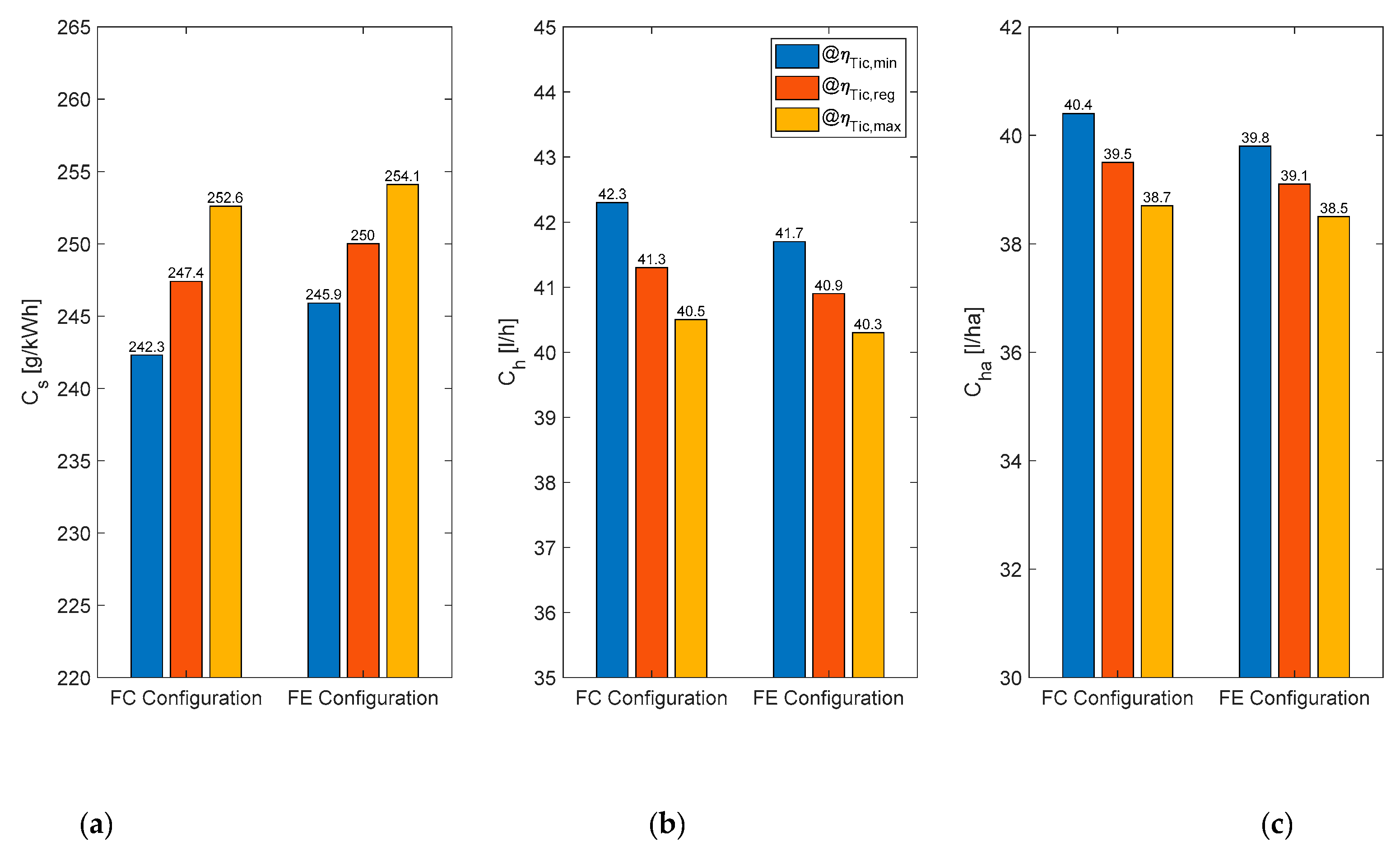
The operational parameters that allow the assessment of the cost-effectiveness of the MC are reported in Table 10 and in the bar graphs in Figure 10.
Considering the specific fuel consumption (Figure 10a), it can be observed that in both FC and FE configurations the values slightly increase, shifting from the lower prediction bound for ηT to the regression model to the upper prediction bound. This is due to the engine characteristic curve (Equation (12)): albeit ne is the same, different values of ηT result in different working points of the engine in terms of torque Te and engine power Pe (Table 10), and, ultimately, in different values of the specific fuel consumption. The fact that the engine working point changes also affects the hourly fuel consumption estimation (Equation (13)), which exhibits an opposite trend with respect to Cs.
A comparison of the fuel consumption between FC and FE configurations shows no significant differences. For example, comparing the values of Cs determined using the regression equation, consumption for the FE configuration is only 1% higher than that for the FC configuration. Even considering the hourly fuel consumption Ch, no significant differences arise; for the FE configuration, Ch is only 0.4 L/h (1%) lower than the one in the FC configuration. A similar trend is found for Cha (the difference between the two configurations is 0.4 L/ha, i.e., 1%). This is due to the fact that Cha is proportional to Ch.
Even considering the most advantageous possible scenario, where consumption is estimated using the traction efficiency upper prediction bound for the FE configuration and the lower prediction bound for the FC configuration, differences remain limited. Indeed, in the FE configuration, Ch is 2 L/h (4.7%) lower and Cha is 1.9 L/ha (4.7%) lower than in the FC configuration. Moreover, if the opposite scenario is considered, where consumption is estimated using the traction efficiency lower prediction bound for the FE configuration and the upper prediction bound for the FC configuration, results are the opposite (Ch and Cha higher in FE configuration than in FC).

4. Discussion and Conclusions

As it concerns the effect of the use of a mechanical ballast position adjustment device such as the MC on the tractive performance, the analysis conducted in this study using exponential regression models shows that there is a non-monotonous trend of the ηT with respect to tractor mass distribution. However, a more detailed analysis conducted on the basis of the overlaps in the model prediction bound areas shows that there are significant overlaps; hence, it does not seem possible to draw reliable conclusions on the beneficial or detrimental effects of the use of the MC on traction efficiency. Theoretical [19,26,37] and experimental [4,5,38] studies have proved that ηT is influenced by the tractor static mass distribution. However, devices such as the MC are able to change the mass distribution by an amount that is insufficient to experimentally observe any effects. Changes in the mass distribution could be amplified by using a heavier ballast; however, this solution could not be applied in this study, since the weight on the front axle in the FE configuration was close to the maximum value allowed by the manufacturer.
Furthermore, the same analysis performed on the net traction ratio indicates that no significant effects of the use of the MC are observable; considering both the regression models and the overlaps in the prediction bound areas, performance in the three configurations (FE, FC and R) are very similar to one another. Indeed, this is a consequence of the fact that the maximum reachable value of net traction ratio is mainly dependent on the total mass of the tractor and the total footprint of the tires [17,39], which were constant in all the three tested configurations and do not change considerably using devices such as the MC.
As it regards the impact of the use of the MC in the economy of farming, a comparison in terms of fuel saving during a simulated common agricultural operation (ploughing) showed no significant effects. Indeed, fuel consumption is strictly correlated to ηT [40] and even considering the best-case scenario where the difference between the ηT in the FE and FC configurations is the maximum that the regression models can indicate, fuel hourly and per-hectare consumptions in the FE configuration are only 4.7% lower (i.e., 2.1 L/h and 1.9 L/ha lower) than those in the FC configuration.
The analysis could be extended by applying the same methodology proposed in this paper to the analysis of other agricultural operations, or by assessing the effects of devices such as the MC on tractor handling. This could be performed by installing an inertial measuring unit (IMU) on the tractor and examining the steering wheel corrections performed by the driver.
In conclusion, the reported results indicate that the changes in tractor mass distribution achievable by mechanical ballast position devices such as the MC do not produce sensible effects on tractive performance and fuel consumption. It thus appears more convenient to address the challenge by acting concurrently on other influential parameters like the tire pressure, choice of the front-to rear wheels combination, and lead of the front wheels, accordingly to what is also observed by other studies in the literature [6,10,41,42,43,44]. Indeed, a tractor able to change all the aforementioned setup parameters depending on the agricultural operation and the soil conditions could reach more significant improvements in terms of efficiency and fuel consumption.

Author Contributions

Conceptualization, M.V., M.M. (Michele Mattetti), M.M. (Mirko Maraldi) and G.M.; Methodology, M.V., M.M. (Michele Mattetti) and M.M. (Mirko Maraldi); Formal Analysis, M.V.; Investigation, M.V., M.M. (Michele Mattetti) and M.M. (Mirko Maraldi); Data Curation, M.V.; Writing—Original Draft Preparation, M.V.; Writing—Review & Editing, M.V., M.M. (Michele Mattetti) and M.M. (Mirko Maraldi); Supervision, G.M. All authors have read and agreed to the published version of the manuscript.

Funding

This research received no external funding

Acknowledgments

This research was supported by ALI s.r.l. (Anghiari, AR, Italy) who provided the Multiplier Counterweight used for the experimental activities.

Conflicts of Interest

The authors declare no conflict of interest.

Appendix A

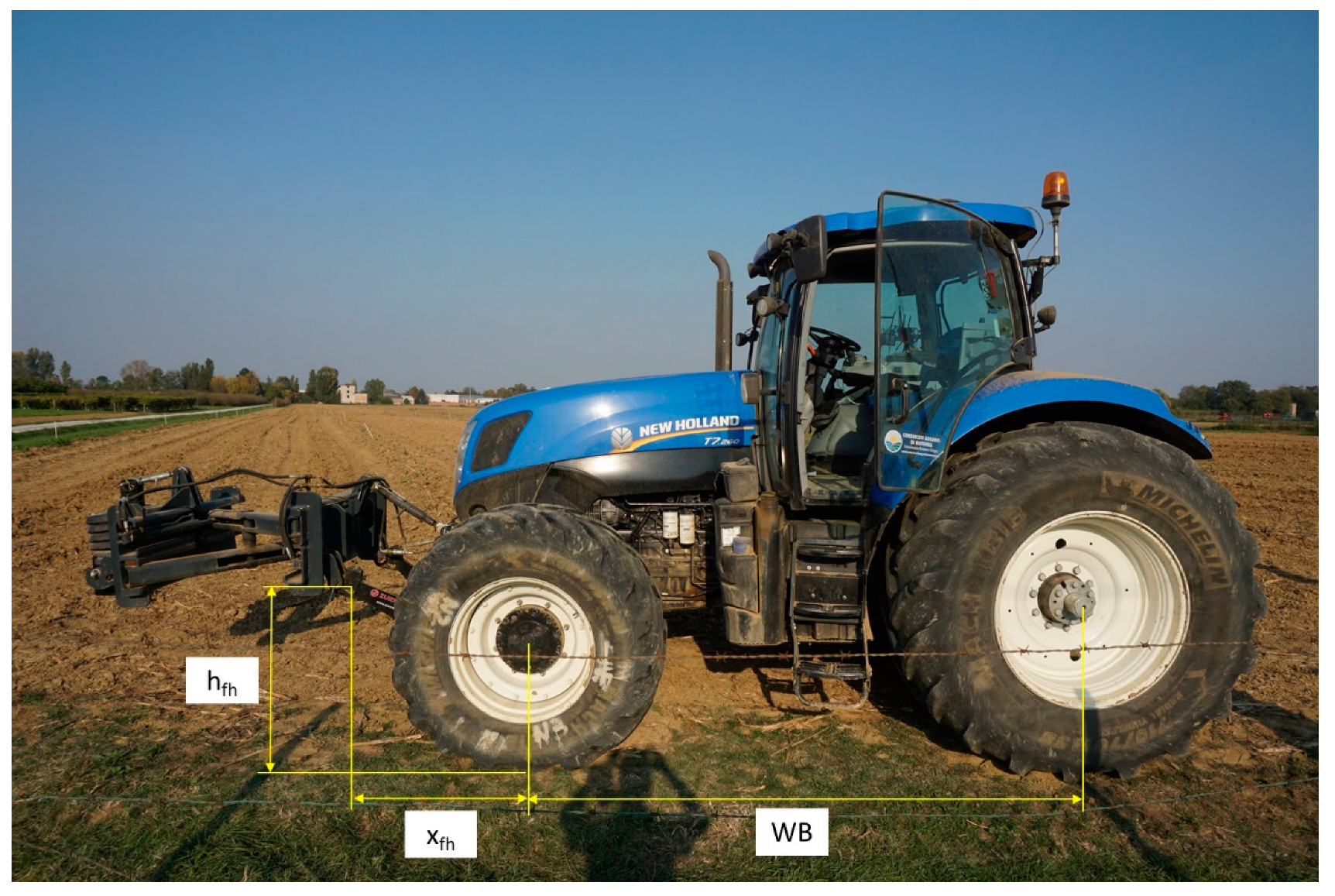
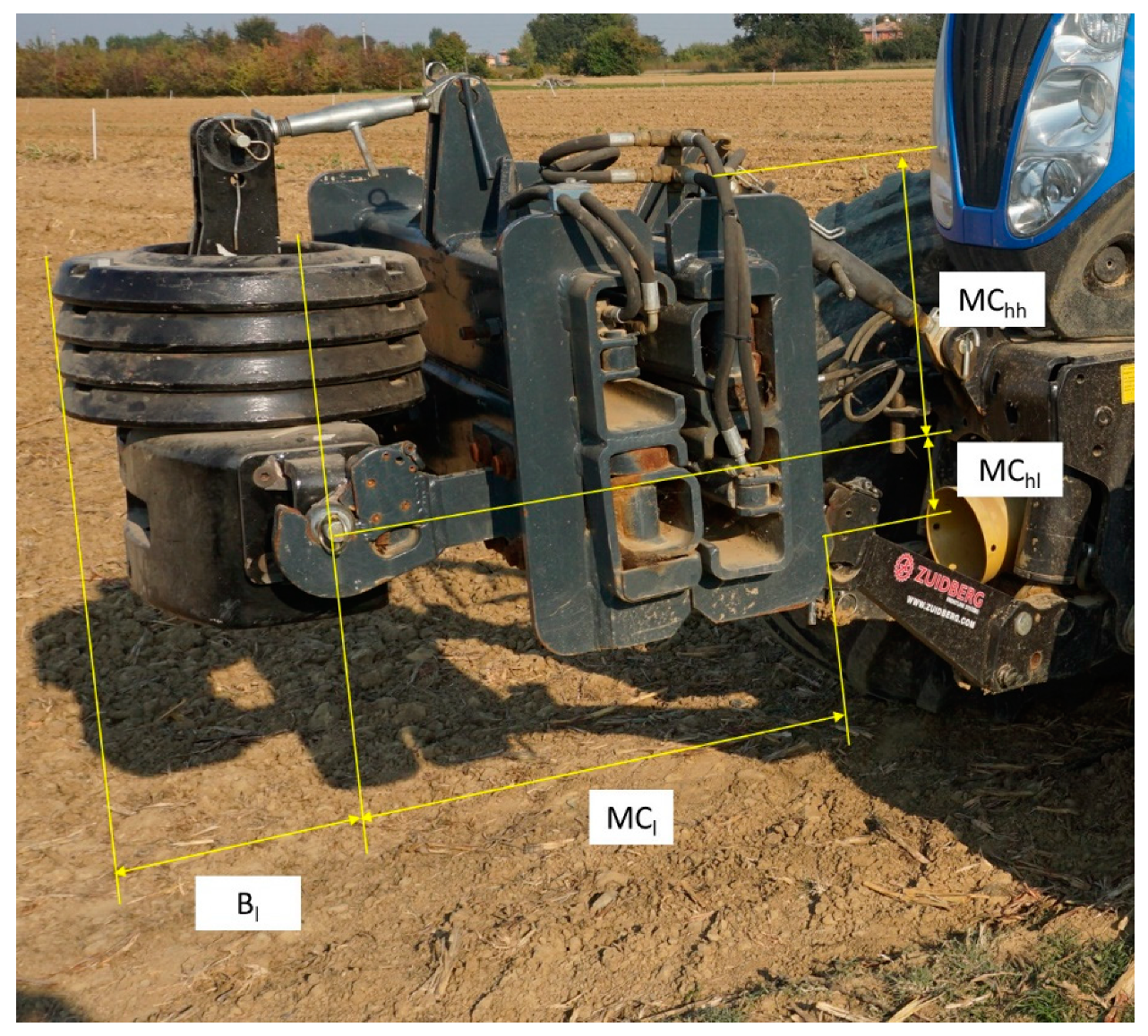
Schematics for the calculation of tractor mass distribution in FE, FC and R configurations are reported in Figure A1, Figure A2 and Figure A3. The dimensions are reported in Table A1.
Figure A1. Tractor dimensions in FC and FE configurations.
Agronomy 10 01820 g0a1
Figure A2. Tractor dimensions in R configurations.
Agronomy 10 01820 g0a2
Figure A3. Multiplier Counterweight and ballast dimensions.
Agronomy 10 01820 g0a3
Table A1. Dimensions for FC, FE and R configurations.
ParameterValue (mm)
Wheelbase (WB)2884
Longitudinal distance of the front hitch from the front wheel hubs (xfh)1665
Height above ground of the front hitch (hfh)850
Longitudinal distance of the rear hitch from the rear wheel hubs (xrh)1200
Height above ground of the rear hitch (hrh)655
Longitudinal length of the ballast over the rear hitch (xrb)400
Longitudinal length (hitch to hitch) of the MC (MCl)690 in FC
1690 in FE
Longitudinal length of the ballast over the MC hitch (Bl)280
Vertical distance between tractor front lower hitch and MC lower hitch (MChl)120
Vertical distance between tractor front upper hitch and MC lower hitch (MChh)480

Appendix B

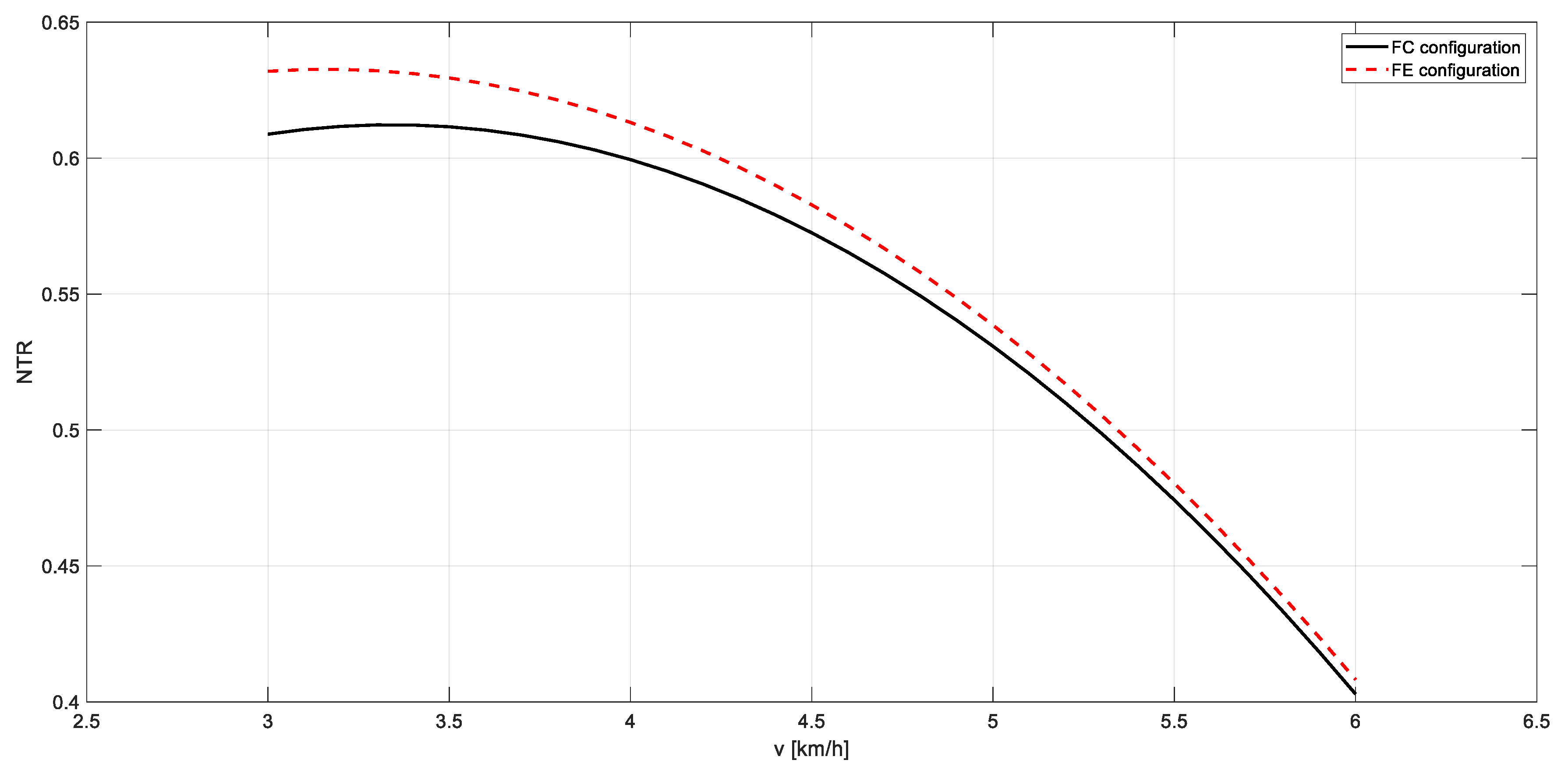
The NTR-v regression curves (E1) obtained from the field tests performed in 8th gear in FC and FE configurations are shown in Figure A4, while the regression parameters are shown in Table A2.
Figure A4. NTR-v regression curves(E1)obtained from the field tests performed in 8th gear in FC and FE configurations.
Agronomy 10 01820 g0a4
Table A2. Regression parameters for the NTR-v relationship in 8th gear.
Regression ParametersFCFE
Coefficient p1
(with 95% confidence bounds)
−2789
(−3955, −1623)
−2624
(−3838, −1410)
Coefficient p2
(with 95% confidence bounds)
1.864 × 10⁴
(7424, 2.986 × 10⁴)
1.660 × 10⁴
(5432, 2.776 × 10⁴)
Coefficient p3
(with 95% confidence bounds)
2.645 × 10⁴
(40.67, 5.285 × 10⁴)
3.328 × 10⁴
(9004, 5.755 × 10⁴)
R^20.970.97

Appendix C

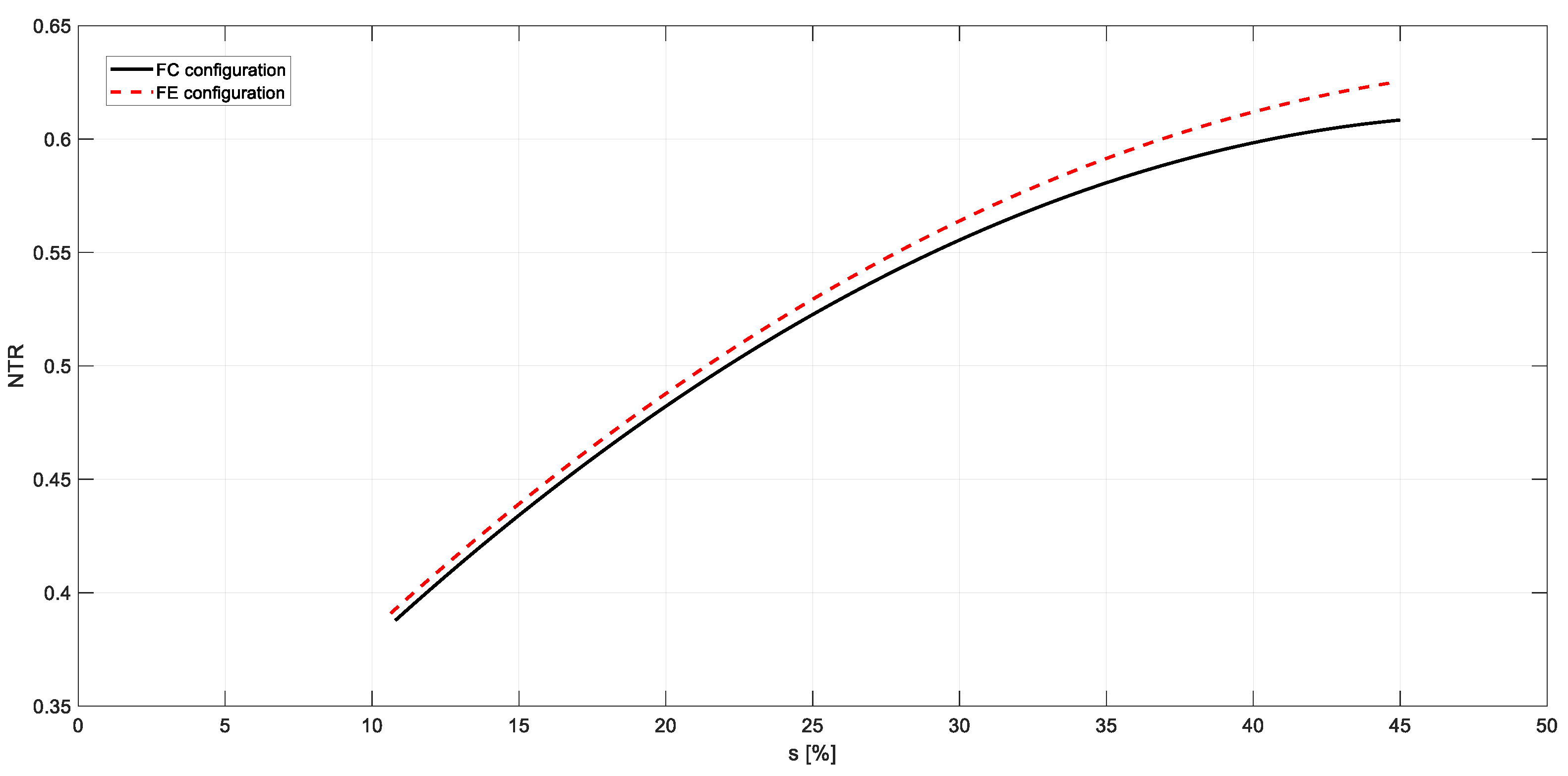
The NTR-s regression curves (E2) obtained from the field tests performed in 8th gear in FC and FE configurations are shown in Figure A5, while the regression parameters are shown in Table A3.
Figure A5. NTR-s regression curves (E2)) obtained from the field tests performed in 8th gear in FC and FE configuration.
Agronomy 10 01820 g0a5
Table A3. Regression parameters for the NTR-s relationship in 8th gear.
Regression ParametersFCFE
Coefficient p1
(with 95% confidence bounds)
−14.31
(−20.65, −7.972)
−13.24
(−19.63, −6.842)
Coefficient p2
(with 95% confidence bounds)
1405
(1032, 1779)
1378
(961.8, 1795)
Coefficient p3
(with 95% confidence bounds)
2.298 × 10⁴
(1.797 × 10⁴, 2.799 × 10⁴)
2.361 × 10⁴
(1.822 × 10⁴, 2.900 × 10⁴)
R^20.970.97

References

  1. Rosenzweig, C.; Hillel, D. Soils and global climate change: Challenges and opportunities. Soil Sci. 2000, 165, 47–56. [Google Scholar] [CrossRef]
  2. Olesen, J.; Bindi, M. Consequences of climate change for European agricultural productivity, land use and policy. Eur. J. Agron. 2002, 16, 239–262. [Google Scholar] [CrossRef]
  3. Kutzbach, H.D. Trends in Power and Machinery. J. Agric. Eng. Res. 2000, 76, 237–247. [Google Scholar] [CrossRef]
  4. Gu, Y.; Kushwaha, R. Dynamic load distribution and tractive performance of a model tractor. J. Terramechanics 1994, 31, 21–39. [Google Scholar] [CrossRef]
  5. Bashford, L.L.; Woerman, G.R.; Shropshire, G.J. Front Wheel Assist Tractor Performance in Two and Four-Wheel Drive Modes. Trans. ASAE 1985, 28, 23–29. [Google Scholar] [CrossRef]
  6. Botta, G.F.; Jorajuria, D.; Draghi, L. Influence of the axle load, tyre size and configuration on the compaction of a freshly tilled clayey soil. J. Terramechanics 2002, 39, 47–54. [Google Scholar] [CrossRef]
  7. Battiato, A.; Diserens, E. Tractor traction performance simulation on differently textured soils and validation: A basic study to make traction and energy requirements accessible to the practice. Soil Tillage Res. 2017, 166, 18–32. [Google Scholar] [CrossRef]
  8. Burt, E.C.; Lyne, P.W.L.; Meiring, P.; Keen, J.F. Ballast and Inflation Effects on Tire Efficiency. Trans. ASAE 1983, 26, 1352–1354. [Google Scholar] [CrossRef]
  9. Serrano, J.M.; Peça, J.O.; Silva, J.R.; Márquez, L. The effect of liquid ballast and tyre inflation pressure on tractor performance. Biosyst. Eng. 2009, 102, 51–62. [Google Scholar] [CrossRef]
  10. Khalid, M.; Smith, J. Axle torque distribution in 4WD tractors. J. Terramechanics 1981, 18, 157–167. [Google Scholar] [CrossRef]
  11. Jadhav, P.P.; Sharma, A.K.; Wandkar, S.V.; Gholap, B.S. Study of tractive efficiency as an effect of ballast and tire inflation pressure in sandy loam soil. Agric. Eng. Int. CIGR J. 2013, 15, 60–67. [Google Scholar]
  12. Özarslan, C.; Erdogän, D. Optimization of tractor plowing performance. AMA Agric. Mech. Asia Afr. Lat. Am. 1996, 27, 9–12. [Google Scholar]
  13. Burt, E.C.; Bailey, A.C.; Patterson, R.M.; Taylor, J.H. Combined Effects of Dynamic Load and Travel Reduction on Tire Performance. Trans. ASAE 1979, 22, 40–45. [Google Scholar] [CrossRef]
  14. Bloome, P.D.; Summers, J.D.; Khalilian, A.; Batchelder, D.G. Ballasting Recommendations for Two-Wheel and Four-Wheel Drive Tractors [Tractor Performance], Microfiche Collection. 1983. Available online: http://agris.fao.org/agris-search/search.do?recordID=US8528799 (accessed on 4 April 2018).
  15. Wismer, R.D.; Luth, H.J. Off-Road Traction Prediction for Wheeled Vehicles. Trans. ASAE 1974, 17, 8–10. [Google Scholar] [CrossRef]
  16. Brixius, W.W. Traction Prediction Equations for Bias Ply Tires, American Society of Agricultural Engineers (Microfiche Collection) (USA). 1987. Available online: http://agris.fao.org/agris-search/search.do?recordID=US8843391 (accessed on 4 April 2018).
  17. Wong, J.Y.; McLaughlin, N.B.; Knezevic, Z.; Burtt, S. Optimization of the tractive performance of four-wheel-drive tractors: Theoretical analysis and experimental substantiation. Proc. Inst. Mech. Eng. Part D J. Automob. Eng. 1998, 212, 285–297. [Google Scholar] [CrossRef]
  18. Zoz, F.M. Predicting Tractor Field Performance (Updated), American Society of Agricultural Engineers (Microfiche Collection) (USA). 1987. Available online: http://agris.fao.org/agris-search/search.do?recordID=US8843392 (accessed on 6 April 2018).
  19. Regazzi, N.; Maraldi, M.; Molari, G. A theoretical study of the parameters affecting the power delivery efficiency of an agricultural tractor. Biosyst. Eng. 2019, 186, 214–227. [Google Scholar] [CrossRef]
  20. Stoilov, S.; Kostadinov, G.D. Effect of weight distribution on the slip efficiency of a four-wheel-drive skidder. Biosyst. Eng. 2009, 104, 486–492. [Google Scholar] [CrossRef]
  21. Osinenko, P.V.; Geissler, M.; Herlitzius, T. A method of optimal traction control for farm tractors with feedback of drive torque. Biosyst. Eng. 2015, 129, 20–33. [Google Scholar] [CrossRef]
  22. Damanauskas, V.; Janulevičius, A. Differences in tractor performance parameters between single-wheel 4WD and dual-wheel 2WD driving systems. J. Terramechanics 2015, 60, 63–73. [Google Scholar] [CrossRef]
  23. Janulevičius, A.; Giedra, K. Tractor ballasting in field work. Mechanika 2008, 73, 27–34. [Google Scholar]
  24. Giedra, K.; Janulevičius, A. Tractor ballasting in field transport work. Transport 2005, 20, 146–153. [Google Scholar] [CrossRef] [Green Version]
  25. Pranav, P.; Pandey, K. Computer simulation of ballast management for agricultural tractors. J. Terramechanics 2008, 45, 185–192. [Google Scholar] [CrossRef]
  26. Gee-Clough, D.; Pearson, G.; McAllister, M. Ballasting wheeled tractors to achieve maximum power output in frictional-cohesive soils. J. Agric. Eng. Res. 1982, 27, 1–19. [Google Scholar] [CrossRef]
  27. Zhang, N.; Chancellor, W. Automatic Ballast Position Control for Tractors. Trans. ASAE 1989, 32, 1159–1164. [Google Scholar] [CrossRef]
  28. Molari, G.; Mattetti, M.; Perozzi, D.; Sereni, E. Monitoring of the tractor working parameters from the CAN-Bus. J. Agric. Eng. 2013, 44. [Google Scholar] [CrossRef]
  29. USDA. Soil Mechanichs Level I; National Employee Develoment Staff, Soil Conservation Service, United State Department o Agriculture: Washington, DC, USA, 1987.
  30. ASTM. D7263-09—Standard Test Method for Bulk Density (Unit Weight) and Voids in Aggregate; ASTM International: West Conshohocken, PA, USA, 2009. [Google Scholar]
  31. ASTM. Test Methods for Liquid Limit, Plastic Limit, and Plasticity Index of Soils; ASTM International: West Conshohocken, PA, USA, 2010. [Google Scholar]
  32. Upadhyaya, S.; Chancellor, W.; Wulfsohn, D. Sources of variability in traction data. J. Terramechanics 1988, 25, 249–272. [Google Scholar] [CrossRef]
  33. Mattetti, M.; Varani, M.; Maraldi, M.; Paolini, F.; Fiorati, S.; Molari, G. Tractive performance of Trelleborg PneuTrac tyres. J. Agric. Eng. 2020, 51, 100–106. [Google Scholar] [CrossRef]
  34. Swiler, L.P.; Sullivan, S.P.; Stucky-Mack, N.J.; Roberts, R.M.; Vugrin, K.W. Confidence Region Estimation Techniques for Nonlinear Regression: Three Case Studies; U.S. Department of Commerce National Technical Information Service: Springfield, VA, USA, 2005.
  35. ASAE. D497.7 Agricultural Machinery Management Data; ASAE: St. Joseph, MI, USA, 2015. [Google Scholar]
  36. Zoz, F.; Grisso, R. Traction and Tractor Performance; ASAE: St. Joseph, MI, USA, 2012; Volume 27. [Google Scholar]
  37. Clark, R.L.; Dahua, Z. A Theoretical Ballast and Traction Model for a Wide Span Tractor. Trans. ASAE 1995, 38, 1613–1620. [Google Scholar] [CrossRef]
  38. Self, K.P. Dynamic Load and Wheel Speed Ratio Effects on Four Wheel Drive Tractive Performance, May 1990. Available online: https://shareok.org/handle/11244/20877 (accessed on 3 November 2018).
  39. Wong, J.Y.; Zhao, Z.; Li, J.; McLaughlin, N.; Burtt, S.D. Optimization of the Tractive Performance of Four-Wheel-Drive Tractors—Correlation between Analytical Predictions and Experimental Data. SAE Tech. Paper Ser. 2000. [Google Scholar] [CrossRef]
  40. Jenane, C.; Bashford, L.; Monroe, G. Reduction of Fuel Consumption through Improved Tractive Performance. J. Agric. Eng. Res. 1996, 64, 131–138. [Google Scholar] [CrossRef]
  41. Spagnolo, R.T.; Volpato, C.E.S.; Barbosa, J.A.; Palma, M.A.Z.; De Barros, M.M. Fuel consumption of a tractor in function of wear, of ballasting and tire inflation pressure. Eng. Agrícola 2012, 32, 131–139. [Google Scholar] [CrossRef] [Green Version]
  42. Senatore, C.; Sandu, C. Torque distribution influence on tractive efficiency and mobility of off-road wheeled vehicles. J. Terramechanics 2011, 48, 372–383. [Google Scholar] [CrossRef]
  43. Janulevičius, A.; Pupinis, G.; Lukštas, J.; Damanauskas, V.; Kurkauskas, V. Dependencies of the lead of front driving wheels on different tire deformations for a MFWD tractor. Transport 2015, 32, 23–31. [Google Scholar] [CrossRef] [Green Version]
  44. Charles, S.M. Effects of ballast and inflation pressure on tractor tire performance. Agric. Eng. 1984, 65, 11–13. [Google Scholar]
Figure 1. Multiplier Counterweight in (a) fully extended configuration (FE); (b) fully closed configuration (FC). (c) The test configuration R, where a standard 1000 kg ballast was mounted on the rear three-point hitch. Schematics for the calculation of tractor mass distribution are reported in Appendix A.
Agronomy 10 01820 g001
Figure 2. Drawbar test setup with the TT in the R configuration. The plough on the Case IH Maxxum 115 (LU) tractor was mounted for the sole purpose of making the LU tractor reach the weight necessary to brake the TT.
Agronomy 10 01820 g002
Figure 3. Regression analysis for net traction ratio (NTR) as a function of s for tractor configuration FE. The experimental data points, the regression curve R2 and the upper and lower prediction bounds (95% confidence level) are visible. The yellow-shaded region is the area used for data comparison.
Agronomy 10 01820 g003
Figure 4. Example of the expected working condition of the tractor-plough system for TT in FE configuration and 8th gear.
Agronomy 10 01820 g004
Figure 5. Example of traction efficiency estimation for tractor configuration FE and 8th gear. ηT FE,reg is the estimation based on the regression model; ηT FE,min is based on the lower prediction bound and ηT FE,maxg is based on the upper prediction bound for the model.
Agronomy 10 01820 g005
Figure 6. Example of the tractor slip estimation starting from the expected value of FDplough. Tractor configuration FC and 8th gear.
Agronomy 10 01820 g006
Figure 7. (a) ηT-s regression curves, and (b) prediction bound areas for tractor configurations FE, FC and R. Regression coefficients are listed in Table 7. The lower and upper slip values for the models are 11 and 52%, respectively.
Agronomy 10 01820 g007
Figure 8. (a) NTR-s regression curves and (b) prediction bound areas for tractor configurations FE, FC and R. Regression coefficients are listed in Table 8. The lower and upper slip values for the models are 11 and 52%, respectively.
Agronomy 10 01820 g008
Figure 9. (a) NTR-ηT regression curves and (b) prediction bound areas for tractor configurations FE, FC and R. Regression coefficients are listed in Table 9. The lower and upper net traction ratio values for the models are 0.40 and 0.64, respectively.
Agronomy 10 01820 g009
Figure 10. Predicted values of (a) Cs, (b) Ch and (c) Cha, for tractor configurations FE and FC in 8th gear. For each configuration, the blue, orange and yellow bars refer to estimations determined using, respectively, the lower prediction bound of the model, the regression model R3, and the upper prediction bound of the model.
Agronomy 10 01820 g010
Table 1. Specification of the New Holland T7.260 (TT) used for the field tests.
SpecificationValue/Description
Engine speed at the maximum engine power (nrated) (rpm)2000
Max engine power @ nrated (kW) 191
Max torque (Tmax) @1500 rpm (Nm)1100
Torque @ nrated (Nm)912
Unballasted mass (kg)8590
TransmissionFull Powershift (gears: 19 forward, 6 reverse)
Front tiresMichelin MACHXBIB 600/65 R28 (50 kPa)
speed radius index rf = 0.700 m
Rear tiresMichelin MACHXBIB 710/70 R38 (50 kPa)
speed radius index rr = 0.925 m
Table 2. Tractor static weight distribution over the axles in fully closed (FC), fully extended (FE) and standard ballast on the rear three-point linkage (R) configurations.
Tractor ConfigurationTotal Tractor Mass (M) (kg)Mass on the Front Axle (%)Mass on the Rear Axle (%)
MC Fully Extended (FE)95905941
MC Fully Closed (FC)95905644
Standard ballast on the rear three-point linkage (R) 95903268
Table 3. Gear ratios for tested gears.
GearGear Ratio ( τ )
7th 7.475 × 10⁻³
8th 8.932 × 10⁻³
9th 1.074 × 10⁻²
Table 4. Regression models and interpolation methods.
CurvesFitting MethodModel Equation
ηT as a function of s (R1)Non-linear least squaresηT = a(b s) + c(d s)
NTR as a function of s (R2)Linear least squaresNTR = p1 s2 + p2 s + p3
ηT as a function of NTR (R3)Non-linear least squaresηT = a(b NTR) + c(d NTR)
Table 5. Regression curve for NTR as a function of v (TT in 8th gear).
CurvesFitting MethodModel Equation
NTR as a function of v (E1)
regression curve and parameters are reported in Appendix B
Linear least squaresNTR = p1 v2 + p2 v + p3
Table 6. Regression curves for FDplough as a function of s (TT in 8th gear).
CurvesFitting MethodModel Equation
FDplough as a function of s
(E2)
regression curve and parameters are reported in Appendix C
Linear least squaresFDplough = p1 s2 + p2 s + p3
Table 7. Coefficient values for the ηT-s regression model (R1).
Regression ParametersFEFCR
Coefficient a
(with 95% confidence bounds)
2943
(−1.907 × 10¹², 1.907 × 10¹²)
37.56
(−4.421 × 10⁶, 4.421 × 10⁶)
−2199
(−6.029 × 10¹¹, 6.029 × 10¹¹)
Coefficient b
(with 95% confidence bounds)
1.036 × 10⁻²
(−699.3, 699.3)
1.060 × 10⁻²
(−10.33, 10.36)
1.366 × 10⁻²
(−399.5, 399.5)
Coefficient c
(with 95% confidence bounds)
−2942
(−1.907 × 10¹², 1.907 × 10¹²)
−37.06
(−4.421 × 10⁶, 4.421 × 10⁶)
2200
(−6.029 × 10¹¹, 6.029 × 10¹¹)
Coefficient d
(with 95% confidence bounds)
1.036 × 10⁻²
(−699.4, 699.4)
1.077 × 10⁻²
(−10.42, 10.44)
1.366 × 10⁻²
(−399.4, 399.5)
R^20.970.960.94
Table 8. Coefficient values for the NTR-s regression model (R2).
Regression ParametersFEFCR
Coefficient p1
(with 95% confidence bounds)
−1.561 × 10⁻⁴
(−1.839 × 10⁻⁴, −1.284 × 10⁻⁴)
−1.290 × 10⁻⁴
(−1.716 × 10⁻⁴, −8.637 × 10⁻⁵)
−1.761 × 10⁻⁴
(−2.033 × 10⁻⁴, −1.488 × 10⁻⁴)
Coefficient p2
(with 95% confidence bounds)
1.535 × 10⁻²
(1.350 × 10⁻², 1.720 × 10⁻²)
1.313 × 10⁻²
(1.053 × 10⁻², 1.573 × 10⁻²)
1.704 × 10⁻²
(1.555 × 10⁻², 1.860 × 10⁻²)
Coefficient p3
(with 95% confidence bounds)
0.254
(0.228, 0.282)
0.291
(0.255, 0.327)
0.223
(0.203, 0.242)
R^20.970.940.97
Table 9. Coefficient values for the NTR-ηT regression model (R3).
Regression ParametersFEFCR
Coefficient a
(with 95% confidence bounds)
−505.1
(−1.103 × 10¹¹, 1.103 × 10¹¹)
−7.706
(−3.584 × 10⁵, 3.584 × 10⁵)
173.9
(−1.000 × 10⁹, 1.000 × 10⁹)
Coefficient b
(with 95% confidence bounds)
3.769
(−7.257 × 10⁴, 7.258 × 10⁴)
2.710
(−1302, 1307)
2.909
(−6541, 6547)
Coefficient c
(with 95% confidence bounds)
505.3
(−1.103 × 10¹¹, 1.103 × 10¹¹)
8.050
(−3.584 × 10⁵, 3.584 × 10⁵)
−173.6
(−1.000 × 10⁹, 1.000 × 10⁹)
Coefficient d
(with 95% confidence bounds)
3.769
(−7.256 × 10⁴, 7.257 × 10⁴)
2.660
(−1284, 1289)
2.912
(−6545, 6551)
R^20.920.840.90
Table 10. Fundamental parameters of the cost-effectiveness analysis during ploughing.
MC ConfigurationFDplough (kN)NTRploughv (km/h)s
(%)
Π (ha/h)ηTPe
(kW)
FC43.40.465.617.71.05ηT FC,min = 0.45
ηT FC,reg = 0.48
ηT FC,max = 0.50
148@ ηT FC,min
142@ ηT FC,reg
136@ ηT FC,max
FE43.90.475.617.71.05ηT FE,min = 0.47
ηT FE,reg = 0.49
ηT FE,max = 0.51
144@ ηT FE,min
139@ ηT FE,reg
135@ ηT FE,max
Publisher’s Note: MDPI stays neutral with regard to jurisdictional claims in published maps and institutional affiliations.