Article

Statistical Analysis versus the M5P Machine Learning Algorithm to Analyze the Yield of Winter Wheat in a Long-Term Fertilizer Experiment

by
Thi Huyen Thai
1,2,3,*,
Richard Ansong Omari
1,2,
Dietmar Barkusky
1 and
Sonoko Dorothea Bellingrath-Kimura
1,2,*
1
Leibniz Centre for Agricultural Landscape Research (ZALF), Eberswalder Str. 84, 15374 Müncheberg, Germany
2
Faculty of Life Science, Humboldt University of Berlin, Albrecht-Thaer-Weg 5, 14195 Berlin, Germany
3
Faculty of Agronomy, University of Agriculture and Forestry, Hue University, 102 Phung Hung Street, Hue 530000, Vietnam
*
Authors to whom correspondence should be addressed.
Agronomy 2020, 10(11), 1779; https://doi.org/10.3390/agronomy10111779
Submission received: 22 October 2020 / Revised: 7 November 2020 / Accepted: 8 November 2020 / Published: 13 November 2020

Abstract

:
To compare how different analytical methods explain crop yields from a long-term field experiment (LTFE), we analyzed the grain yield of winter wheat (WW) under different fertilizer applications in Müncheberg, Germany. An analysis of variance (ANOVA), linear mixed-effects model (LMM), and MP5 regression tree model were used to evaluate the grain yield response. All the methods identified fertilizer application and environmental factors as the main variables that explained 80% of the variance in grain yields. Mineral nitrogen fertilizer (NF) application was the major factor that influenced the grain yield in all methods. Farmyard manure slightly influenced the grain yield with no NF application in the ANOVA and M5P regression tree. While sources of environmental factors were unmeasured in the ANOVA test, they were quantified in detail in the LMM and M5P model. The LMM and M5P model identified the cumulative number of freezing days in December as the main climate-based determinant of the grain yield variation. Additionally, the temperature in October, the cumulative number of freezing days in February, the yield of the preceding crop, and the total nitrogen in the soil were determinants of the grain yield in both models. Apart from the common determinants that appeared in both models, the LMM additionally showed precipitation in June and the cumulative number of days in July with temperatures above 30 °C, while the M5P model showed soil organic carbon as an influencing factor of the grain yield. The ANOVA results provide only the main factors affecting the WW yield. The LMM had a better predictive performance compared to the M5P, with smaller root mean square and mean absolute errors. However, they were richer regressors than the ANOVA. The M5P model presented an intuitive visualization of important variables and their critical thresholds, and revealed other variables that were not captured by the LMM model. Hence, the use of different methods can strengthen the statement of the analysis, and thus, the co-use of the LMM and M5P model should be considered, especially in large databases involving multiple variables.

1. Introduction

Winter wheat (WW) (Triticum aestivum L.) is an important cereal in Europe and accounts for over 32% of the total global production next to Asia [1]. In Germany, WW covers 3.2 million hectares, accounting for around one-third of the total arable land area. The average total WW production from 2014 to 2018 was 24.7 million tons, with an average yield of 7.7 t ha−1 [2]. The grain yield of WW in Germany has increased in recent decades from an average of less than 3 t ha−1 in the 1960s to around 8 t ha−1 in the 2000s [1]. However, the grain yield of WW has fluctuated in recent years. Apart from crop breeding improvement, which has contributed dramatically to the wheat yield increase throughout the 20th century in Germany [3,4], several other factors, such as enhanced agronomic management, favorable weather conditions, and soil improvement, also played an important role in yield development and yield stability [5,6]. Thus, similar to other crops, yield variation in WW is the result of interdependencies and complex interactions among different factors. In this regard, identifying the major factors and their relationships that account for grain yield variation of WW is crucial to understanding how to maximize yields and minimize annual yield fluctuations each year.
Long-term field experiments (LTFEs) provide insight to unravel the factors that influence crop yield dynamics in different cropping systems and thus serve as a means to assess the sustainability of agricultural practices over time [7]. Northeast Germany is one of the driest regions in central Europe, with loamy and sandy soils being the two dominant soil types [8,9]. Cereals are one of the main crops cultivated in this region. Previous cereal crop-related long-term experiments in the region have focused on crop yields [10,11], tillage [12], and the soil organic carbon (SOC) [13]. Moreover, irrespective of the underlying drought stress and poor water holding conditions of the prevailing soils in large areas of the northeast, concerns over climate change have driven research in these environments [14,15].
In analyzing data from designed experiments, classical parametric methods such as the analysis of variance (ANOVA), parametric correlation, and regression have long been commonly used to assess crop yield [16]. However, these classical methods have limitations. For example, while ANOVA is best suited to identifying yield differences between treatments in designed experiments, it does not exhaustively account for the extraneous factors that influence yields [17,18]. Similarly, parametric correlations and linear regressions are less suited to handle missing, unbalanced, and higher-order data and nonlinear interactions [18,19]. Flexible and robust methods are now available for dealing with multivariate, unbalanced data that account for nonlinear, higher-order interactions. For instance, statistical models such as the linear mixed-effects model (LMM), generalized linear models [20,21], and machine learning (ML) models such as random forest, artificial neural networks, and decision tree algorithms [22,23,24] can be applied to handle these challenges. Unlike ANOVA models, LMMs cover nontreatment variables and random factors that tend to mask the treatment effects, thereby improving the reliability and interpretation of experimental results [18]. While Piepho [25] stated that the most common variables affecting the yield could be determined in the LMM framework when environmental effects and treatment effects are considered random and fixed factors, other reports advised that the LMMs and linear regression models have limitations because the analytical interpretation and pattern prediction can be confounded due to significant high autocorrelation or missing data [26,27,28]. ML models such as the classification and regression tree (CART) and M5P algorithm-based decision tree have been employed in agricultural research [29,30]. These regression tree models are most useful in handling complex databases with a high number of attributes and high dimensions collected from observational experiments [31] but can also profitably be applied for small datasets from designed experiments [32]. They are robust tools for dealing with missing data. Additionally, regression tree models can capture important nonlinear relationships and interactions between variables [31]. However, this method, by contrast, has not yet been widely used in analyzing data collected from LTFEs.
Statistical inference and prediction are two major goals in the study of agricultural experiments. While statistical models are designed to draw inferences of relationships between variables within assumptions, ML is a modeling tool for finding generalizable predictive patterns without hypotheses [33]. Limitations in the use of statistical inferences and ML are still subject to debate. We have not yet found clarity in the literature regarding the comparison of how different statistical analyses and the ML model explain the results of LTFE data. Moreover, it is important to know the best suited tools and methods for unraveling the important interconnected multiple variables that influence crop yields in the long term. Therefore, in this study, we tested the use of ANOVA in the general linear model and two nonparametric methods, the LMM and M5P models, to understand grain yield variations of WW in an LTFE (“V140”) in Müncheberg, Germany. The objectives of the study were to (1) identify the important variables that explain the grain yield variations of WW in the LTFE and (2) compare different analytical methods for explaining the WW yield variation.

2. Materials and Methods

2.1. Experimental Site

The LTFE “V140” was established at the experimental station of the Leibniz Centre for Agricultural Landscape Research (ZALF), Müncheberg, Germany, in 1963 [34]. The site is located in the Märkisch-Oderland district, around 50 km east of Berlin. The area is characterized by a dry period, particularly during the early summer [35]. The mean annual precipitation in the area was 551 mm ± 121.6 standard deviation (s.d.), and the mean annual temperature was 8.7 °C ± 0.9 s.d. during the cultivation period of WW (1973–2010). The soil in the area is classified as a Podzoluvisol to Arenosol. According to the German Guidelines for Soil Assessment (Bodenschätzung), the dominant soil texture classes are slightly loamy sand and sand (Sl4D and S4D) [34]. The site has recently been described in more detail in Thai et al. [36].

2.2. Experimental Design and Management

The experiment was set up on a flat plain measuring 5712 m2 involving 168 individual plots. The individual plots measured 6.0 m × 5.0 m, and a buffer zone of 1 m was allowed between the blocks. The experiment was arranged in a randomized complete block design (RCBD) comprising 21 treatments with eight blocks. The treatments included five levels of mineral N fertilizer (NF), each in combination with four organic fertilizers (ORF) (Table S1, supplementary). The five NF levels comprised 35, 70, 105, 140, and 175 N kg ha−1, which are hereafter referred to as N1, N2, N3, N4, and N5, respectively. The ORF treatment included 0, 1.2, and 3.2 t dry mass (DM) ha−1 farmyard manure (FYM) and 2.0 t DM ha−1 straw, which is henceforth referred to as sole mineral fertilizer (nitrogen, phosphorus, and potassium combination), fym1, fym2, and straw applications, respectively (Table S1). However, at a 3.2 t DM ha−1 application rate of FYM, the NF levels applied were 0, 35, 70, 105, and 140 N kg ha−1 (fym2 application). The control treatment received no fertilizer inputs. Due to the different NF levels in the fym2 application compared to other applications, group treatments were made to balance the NF rates among the different applications to compare the effects of different ORFs on the yield. The group treatments included control, NPK, NPK + fym1, NPK + fym2, PK + fym2, and NPK + straw (Table S1, supplementary material). From 1980 onwards, phosphorus and potassium fertilizers were applied at 30 kg P2O5 ha−1 and 100 kg K2O ha−1, respectively, to all plots except the control treatment. NF was applied twice each year during the growth of WW, i.e., the basal amount was applied in the middle of April, and the remainder was applied a month later between shooting to full blooming (end of May or early June). The FYM was applied every two years from 1973 to 1994 in autumn before planting maize, potato, or sugar beets, depending on the cropping system in the year. After 1994, the FYM was applied every four years in autumn before planting maize or potatoes. The FYM used in each year contained, on average, 2.1% N, 0.7% P2O5, 2.1% K2O, 0.4% Mg, and 55.4% organic matter. Straw from the preceding cereal crop was applied at 2 t ha−1 every two years throughout the experimental period. The dry mass straw contained, on average, 0.7% N, 0.1% P2O5, 1.9% K2O, and 0.1% Mg. Lime was uniformly applied to all the plots in all trial years.
Sowing of WW was performed at the end of September or in early to middle October in most years during the study period. The sowing densities were the same in all experimental years, but the WW varieties were changed over time. Harvesting was performed at the end of July or the beginning of August in most experimental years, depending on the weather conditions. The WW was harvested at the physiological maturity stage using a harvester. Weeds were controlled with a postemergence herbicide.
The crop sequence was not fixed and consisted of WW, winter rye, spring barley, potatoes, sugar beets, maize, flax, and peas (Table S2, supplementary). One of these crops was cultivated in the experimental site during each growing season. The crop preceding WW was potatoes in 1973, 1983, 1987, and 1991 and sugar beets in 1993. In 2001 and 2009, the crop preceding WW was peas. There were seven WW crop rotations, and the crop rotations were different in this experiment. The management practices of WW, such as plowing, harrowing, and fertilization, were the same in each experiment year.

2.3. Data Description

Crop yield: Long-term data from 1973 to 2010 were used for the analyses. The DM grain yield data of WW (Mg DM ha−1) were obtained from the seven years of WW cultivation. The DM yield of the preceding crop was obtained in each trial year to estimate its effects on the yield of WW.
Meteorological data: The weather data used in the analysis were obtained from an adjacent climate station of the German Meteorological Service [37]. The daily mean air temperature, maximum temperature, minimum temperature, and precipitation during the growing period of WW were used to calculate the input weather variables for this study. The monthly mean temperature, cumulative precipitation, cumulative number of days recorded with mean temperatures above 30 °C in every month (days Tmax > 30 °C in a month), the cumulative number of days recorded with mean temperatures below 0 °C or 32 °F (freezing days in a month), and cumulative growing-degree days during the growing seasons were calculated. The maximum and minimum temperatures were used to calculate the growing degree days (GDD).
Soil variables: Soil chemical analyses were performed in the 1984, 1988, 1992, and 1994 trial years. The results of the soil analysis are presented in Table S3 of the supplementary material. Selected soil variables such as the total N and SOC in each treatment were used as input data to estimate their effects on the yield of WW. All input variables considered in this study are presented in Table S4 of the supplementary material.

2.4. Data Analysis

There are two main steps in the analysis: (1) exploring the WW grain yield and yield variability using descriptive analysis and ANOVA within fixed effects models-general linear model and (2) applying nonparametric methods involving the LMM (statistical model) and M5P (ML model) models for the grain yield response.

2.4.1. ANOVA Test

The effects of fertilization treatments on the grain yields were analyzed by one-way ANOVA using SPSS version 25, and the significance was determined by Tukey’s post hoc test. A fixed-effects model, the general linear model, was used to evaluate the main and interaction effects among treatments (fertilizer) and years (annual or environmental effects) on the grain yields over the years. The effect sizes of the fertilizer, environmental factors, and their interactions were estimated based on the sum of squares-type III in the general linear model. The environmental factors considered in this study were weather, soil chemical properties, and preceding crops and their yields. Furthermore, soil data were analyzed by ANOVA to understand the changes in soil properties under long-term fertilization practices and then to select the important variables for developing models. To avoid the effects of collinearity in the statistical model and overfitting in the ML model, Pearson’s correlation analysis was checked between the target variables (WW grain yield) and predictor variables and between predictor variables together. Based on Pearson’s correlation coefficient, useful variables were maintained, while redundant variables were removed before developing the yield models. Statistical significance for the analyses was set at p < 0.05.

2.4.2. Linear Mixed-Effects Models

LMMs are an extension of the linear regression model and include both fixed and random effects as predictor variables via a restricted maximum-likelihood estimate (REML). The LMMs were fitted using the “lmer” function implemented in the “lme4” package [20] of the R statistical language, version 3.6.3 [38], to assess the WW yield as a function of the different factors. The LMM for the yield response is specified by Equation (1).
y = Xβ + Zu + ε
Here, y is the vector of the wheat yield (outcome/target variable: Mg ha−1); X and β are the design matrix and the vectors of fixed effects, respectively; Z and u are the design matrix and the vectors of random effects; and ε represents the vector experimental error. In this study, the LTFE with RCBD was specified with experimental years and experimental blocks and plots as random effects on the yield. The fixed-effect variables were the levels of NF, type, and levels of ORF, selected weather parameters, preceding crops and their yields, and selected soil chemical properties. Regarding the model development process, after checking for normality on model residuals using quantile-quantile (Q–Q) plots, we first fitted the random effect model. Then, we added more predictors as fixed effects to the random effect model. From these LMMs, we performed gradual backward elimination of nonsignificant LMM effects, beginning with the random effects followed by the fixed effects. In this study, the LMM was fitted as a random intercept model at a 97.5% confidence interval (CI). Models were selected using the Akaike Information Criterion (AIC).
From the final LMM, we calculated the relative important variables using the Relaimpo package in R, version 3.6.3 [39]. This is a supplemental test to regression analysis to calculate the proportional contribution of each predictor variable to explaining variance in the LMM. The statistical tests were considered significant at the 0.05 probability level.

2.4.3. Machine Learning Model

We used the M5P algorithm, which is a recursive partitioning algorithm based on thresholds for developing a decision tree structure, to uncover the relationship and interaction between the WW yield and predictor variables. The M5P is a powerful implementation of Quinlan’s M5 algorithm [40,41] and an advantaged algorithm among decision tree algorithms for training an ML model. We implemented M5P in WEKA (Waikato Environment for Knowledge Analysis) software version 3.8.4. The rule of M5P is to recursively partition the data space and fit a prediction model within each partition. The results of the implementation are a binary regression tree model and are represented as an inverted tree, wherein the terminal nodes are the linear regression functions. The tree includes a root node (top node), internal nodes, and terminal nodes connected by edges. Additionally, branches or subtrees are split from the root node, and internal nodes correspond to the outcome of the test. The terminal nodes are the prediction values of the WW yield. When the values of the outcome at the terminal nodes are numeric, the terminal nodes of the tree can be constant values, and the tree is called a regression tree. In contrast, the tree is called a model tree once the terminal nodes of the tree are piecewise linear regression equations [42]. Before training the M5P model, we checked the correlation ranking between the selected input variables and yield by the attribute selection function in WEKA. Next, we used the split function in WEKA to randomly partition the preprocessed data into two subsets, including the training set (80%) and test set (20%). The training set was used to build the decision tree model (determine its parameters), the ten-fold cross-validation method was used to estimate the accuracy of the supervised learning algorithm, and the test set was used to evaluate the predictive performance of the trained model [43]. The coefficients of determination (R2) and root mean square error (RMSE) were used to assess the performance of the models. After obtaining a final M5P model, we used bootstrap 1000-tree analysis by the Relaimpo package in R version 3.6.3 [39], to identify the relative importance of predictor variables. In this study, we present the results of the regression tree model as a piecewise constant function.

2.4.4. Evaluation Metrics

A good fitting model is generally one in which the results of the predicted values are close to the actual values for the selected model. Thus, the predicted grain yields of WW produced by LMM and M5P-based regression trees were compared to the actual yields observed in the LTFE. We employed standard statistical criteria such as R2, RMSE, and mean absolute error (MAE) values to assess the predictive performance for WW grain yields by the selected models. The R2 value indicates the fitness of the model for predicting the WW yield, while the RMSE and MAE are commonly used to measure the difference between the predicted and actual values. Furthermore, the RMSE can be used to evaluate the closeness of these predictions to the actual values, while the MAE can better represent the predictor error. Higher R2 values and lower values of the RMSE and MAE indicate better estimation accuracies of the models [44]. Equations for the evaluation metrics are given in the supplementary material, EQ1 (Es1, Es2, Es3).

3. Results

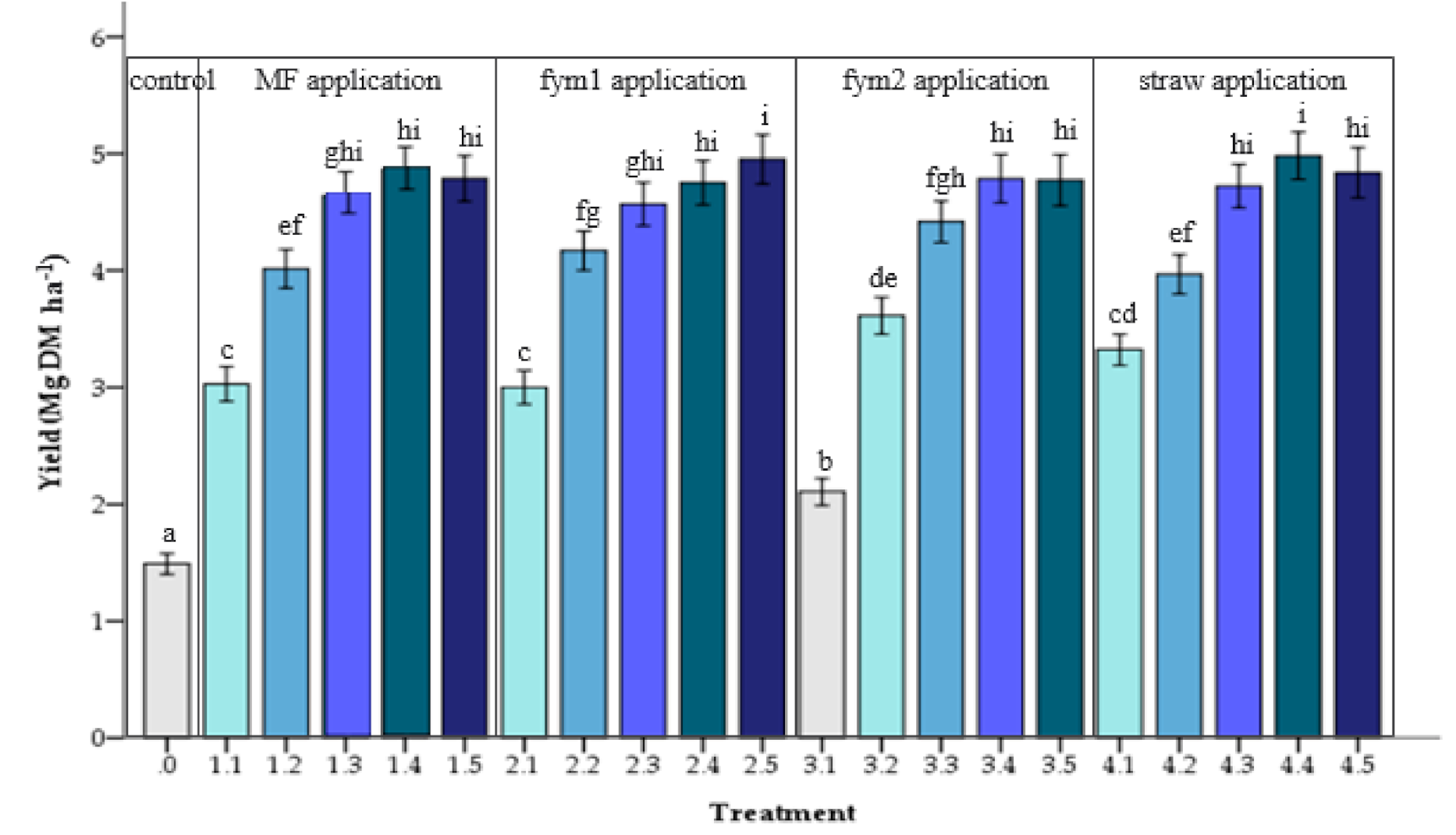
3.1. Grain Yield of Winter Wheat

The ANOVA results show that there was a significant effect of fertilization on the grain yield of WW (Figure 1, p < 0.001). Irrespective of ORF application, the mean grain yield increased significantly with increasing NF application rates until N3, except in fym1 and fym2. At zero NF, treatment 3.1 showed nearly 0.5-times higher increases in grain yield relative to the no input control. At N1, the highest significant mean grain yield was observed when coapplied with fym2, while no differences were observed among mineral fertilizer, fym1, and straw applications. There were no significant differences in mean grain yields among the four application regimes (mineral fertilizer, fym1, fym2, and straw application) at N2, N3, N4, and N5. Optimal mean grain yields of less than 5.0 Mg DM ha−1 were obtained at N3 in the mineral fertilizer and straw application and at N2 in fym1 and fym2 applications. Optimal yields of 4.60 Mg DM ha−1 and 4.16 Mg DM ha−1 were observed at N3 and N2 in mineral fertilizer and fym1 applications, respectively. In fym2 and straw applications, optimal yields of 4.44 Mg DM ha−1 and 4.69 Mg DM ha−1 were obtained at N2 and N3, respectively. Therefore, FYM applications with both levels (fym1 and fym2) showed better effects on the grain yields compared to mineral fertilizer application or straw application.
The mean WW grain yields of the group treatments are shown in Table 1. The average yields ranged from 1.48 Mg DM ha−1 year−1 in the control to 4.42 Mg DM ha−1 year−1 in the NPK + fym2 treatment. The average grain yields were not significantly different among the NPK, NPK + fym1, NPK + fym2, and NPK + straw treatments. The average grain yield in NPK + fym2 was twice as high as that in PK + fym2 and three times higher than that in the control. The coefficient of variation (CV) of grain yields for each group treatment ranged from 0.26 in NPK to 0.39 in the PK + fym2 treatment. Non-NF input treatments (control and fym2 + PK treatments) showed relatively higher CV values of 0.33 and 0.39, respectively, compared to NF-applied treatments. The NF-applied plots showed similar CV values of 0.26 and 0.27. In general, the results of ANOVA and descriptive statistics in Table 1 show that NF treatments can maintain a stable and higher WW grain yield compared to treatments without NF.
The grain yield dynamics of WW in the tested years are shown in Figure 2. Irrespective of the group treatment application, there were significant differences in WW grain yields among the trial years. The WW grain yield variability was high among the years and ranged from 2.35 Mg DM ha−1 in 1991/92 to 5.39 Mg DM ha−1 in 1983/84. Except for the PK + fym2 treatment, there were significant increases in grain yield for all group treatments compared to the control in almost all years.
The results of ANOVA or general linear model analysis show that the grain yield of WW was significantly affected by the environment/year (42%), followed by the fertilization treatment (34%) and environment × fertilization (6%), with 17% of the variation attributed to error (other factors) (Table 2). These results explain 80% of the variance with an adjusted R squared value of 0.80 at p < 0.001.

3.2. Modeling and Predictors

3.2.1. Linear Mixed-Effects Model

The results of the LMM reveal that NF application, freezing days in December and in February, precipitation in June, the yield of the preceding crop, the temperature in October, the cumulative number of days in July with maximum temperatures above 30 °C (days Tmax > 30 °C in July) and the total N in the soil were fixed factors that influenced the grain yield of WW (Table 3). The model indicated blocks and plots as random factors. The fixed effects explained 73% (Rm2 = 0.73) of the variance in the grain yield, while the total of both the fixed and random effects explained 80% of the variance (R2c = 0.80) at a 97.5% CI. In particular, NF application and freezing days in December showed the highest significant contribution to the grain yield, i.e., 21.7% and 17.3%, respectively (Table 4). However, the temperature in October (3.9%) and total N in the soil (3.3%), although significant, were less important predictors of the grain yield. The plots and blocks explained 15.2% and 10.5% of the variance in the grain yield, respectively.

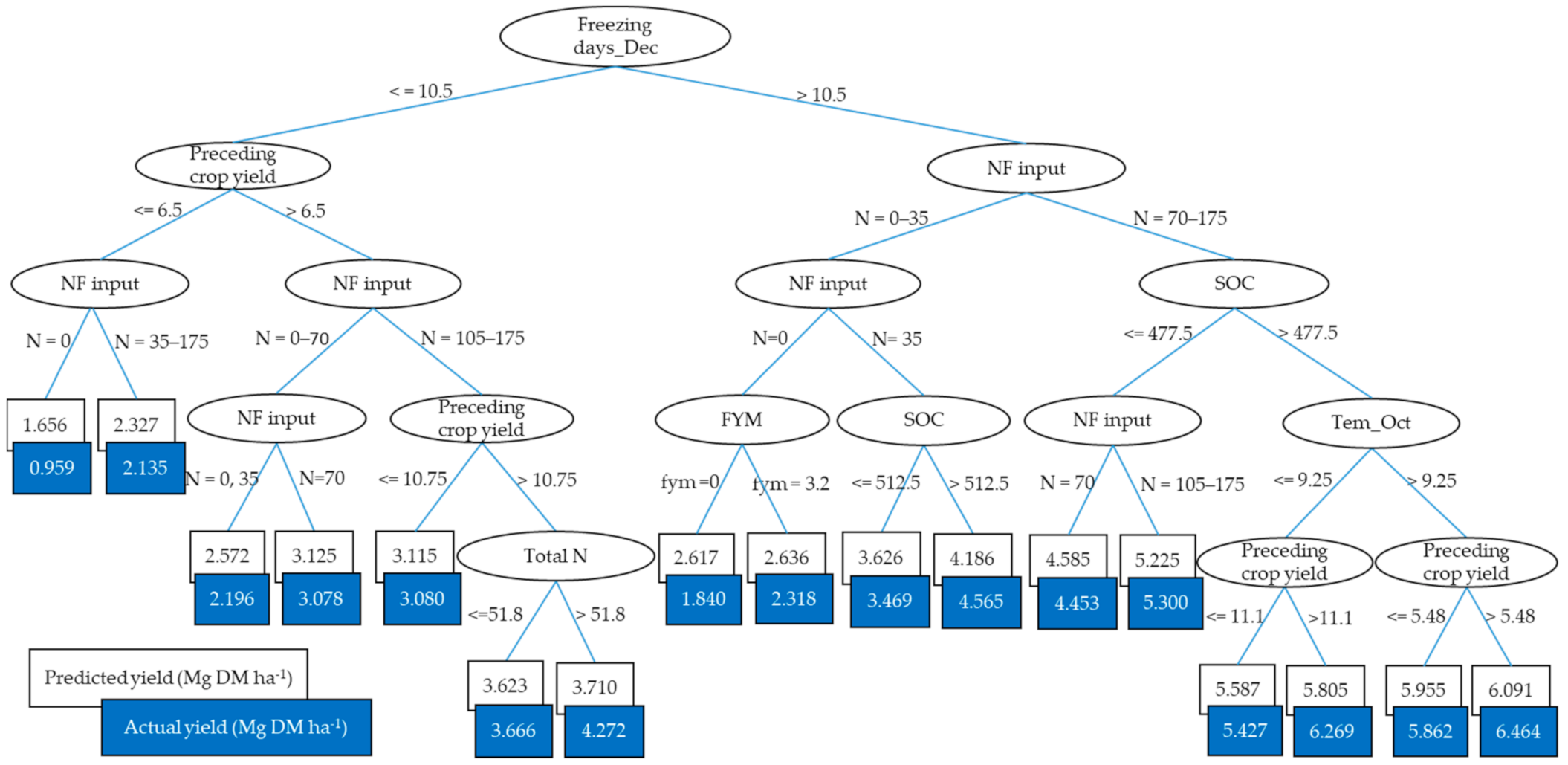
3.2.2. Machine Learning Model

The M5P regression tree model generated five splits and 17 terminal nodes and explained 80% of the variability in the data (Figure 3). The hierarchy of the regression tree model, as well as the results from bootstrapping 1000 trees, indicated freezing days in December and the NF rate as the main determinants of the WW grain yield (Figure 3, Table 4). Freezing days in December and the NF rate accounted for 31.7% and 22.5%, respectively, of the contribution to the grain yield of WW. Other variables, such as the yield of the preceding crop, the temperature in October, freezing days in February, the total N in the soil, the SOC, and the FYM, were also determinants of the WW grain yield. The total N in the soil, SOC, and FYM showed a minimal influence on the grain yield of WW, with relative contributions of 3.0%, 2.3%, and 0.4%, respectively. The effects of the total N in soil and SOC on the grain yield were only evident in plots that received NF application. In contrast, the FYM slightly influenced the grain yield only in plots that received no NF application (Figure 3).

3.2.3. Comparing Models and Model Fit

The results of ANOVA indicate fertilizer application and the environment as the main factors that explained the grain yield, with an adjusted R squared of 0.80 (Table 2). Among the treatment inputs, NF application was the main variable that influenced the grain yield, while FYM slightly influenced the grain yield with no NF application. The effects of fertilizer and the environment on the grain yield were revealed in detail in the results of the LMM and M5P regression tree models. Both the LMM and M5P model identified the NF and freezing days in December as the most crucial variable that influenced the grain yield of WW (Table 4). However, the relative proportions of both variables differed hierarchically in both models. The NF rate was the most important variable, while freezing days in December was the second most important variable that explained WW yields in the LMM. Conversely, the results from the M5P model show the NF rate as the second most important variable and freezing days in December as the first most important predictor of WW yields. Additionally, freezing days in February, the yield of the preceding crop, the temperature in October, and the total N in the soil were determinants of the grain yield in both models. Apart from the common determinants in both models, the LMM highlighted precipitation in June and days Tmax > 30 °C in July, while the M5P model revealed SOC and FYM in plots that received zero NF input as variables that influenced the WW yield.
The results of the fitting model for the LMM (R2 = 0.8, p < 0.001) and the training model for the M5P regression tree (R2 = 0.8) (Table 4) show a generally good fit between the predicted yield and actual yield of WW. The evidence of good fit between the predicted yield (modeled) and actual yield (observed) for the LMM and M5P model are shown in Figures S1 and S2 in the supplementary material. The LMM showed a better performance in predicting the grain yield compared to the M5P regression tree model, as reflected by its relatively smaller RMSE and MAE values. The LMM showed RMSE and MAE values of 0.68 and 0.54, respectively, while 0.74 and 0.58 were computed for the M5P regression tree model.

4. Discussion

4.1. Grain Yield of Winter Wheat and Treatment Effects

The optimum WW grain yield of less than 5.0 Mg DM ha−1 observed in the current study was much lower than the national average yield of 7.7 Mg DM ha−1 from 2014 to 2018 [2]. The yields of WW in this study markedly increased when NF or its combination with ORF was applied (Figure 1). Similar to the observations for spring barley in the experiment [36], we found that NF input was a major determinant of the grain yield of WW. Fixen and West [45] stated that plant-available N is one of the most important nutrients for increased yields of major food crops. In this study, the average grain yields of WW increased to optimal yields along with increasing NF application to a certain threshold. The optimal yields were obtained at N3 in the mineral fertilizer and straw applications and at N2 in the fym1 and fym2 applications (Figure 1). This reveals that the effects of NF application on the yield of WW were different under different ORF applications. The effect of the ORF application compared to mineral fertilizer application alone on the grain yield was evident at N1 only in the fym2 application, reiterating the importance of FYM amendment and its dose in attaining the optimum yields of crops. FYM amendment can reduce the need for the higher NF application rate demanded by wheat. This observation is similar to those in studies by Blanchet et al. [46] in Switzerland.
The combined application of FYM with mineral fertilizer has been reported to improve the grain yield of WW in Germany [11,47]. The yield increase is attributed directly to the effects of additional N and indirectly to the improved soil conditions related to organic material applications [48]. In this study, with the same NF input in NPK, NPK + fym1, NPK + fym2, and NPK + straw, the average yields of these group treatments were similar, irrespective of the ORF application type and amounts (Table 1), implying the minimal influence of FYM or straw on the grain yield. Additionally, the FYM in plots that received zero NF input appeared in the M5P regression model, but the corresponding effect on the WW yield variation was very small. This is ascribed to the fact that organic inputs are usually low in nutrients and unable to satisfy the nutrient demands of cultivated crops [49].
Although the effects of FYM application on the grain yield variation were very small and the effect of straw on the yield was not clear in the present study, the combined application of ORF along with NF increased the grain yield stability of WW (Table 1). These findings are consistent with observations from WW grain yield stability studies in Giessen, Germany [5,6]. We observed higher grain yield stabilities of WW in all treatments with NF input, as shown by their lower CV values compared to the control or PK + fym2 treatment. This observation is ascribed to the plant-available N input from NF, which aided in the vigorous growth of wheat plants and the development of greater resilience against environmental stress. NF was the main fertilizer factor that showed enhanced effects on wheat yields through improvements in plant growth and root development [50], and thus aided in the water and nutrient uptake capacity. Thus, NF application in the WW cultivation system could not only enhance grain yields but also reduce the yield variability year to year.

4.2. Environmental Effect on the Winter Wheat Yield

The temperature in October was an influencing variable for the WW grain yield in both models (Table 4). In this experiment, WW was sown at the end of September to mid-October. In general, the optimal temperature for wheat germination is 12 to 25 °C [51], while the average temperature in October throughout the trial years was 8.7 ± 1.8 °C (Table S5a). Therefore, a warmer temperature in October is favorable for the germination, emergence, and initial growth of leaves, crowns, and secondary root systems of WW plants [52].
Many previous studies have reported on the effects of winter freezing temperatures on the grain yield of WW [53,54,55]. Our findings reveal that freezing days in December appeared to be the most crucial and consistent climate-based driver for the grain yield of WW in both the LMM and M5P model (Table 4). The freezing days in February were also a consistent determinant of grain yields in both models, although they showed only a 7.6% contribution in the LMM and a 4.6% contribution in the M5P model. Seedlings of wheat normally require a minimum of four to five leaves and at least one to two tillers to have enough energy reserves to survive the winter [56]. Thus, winter hardiness or cold tolerance is an extremely crucial physiological process that affects wheat survival during winter and its subsequent growth and development. According to Lollato et al. [56], wheat plants remain cold-hardy as long as the crown temperatures remain below 0 °C. The wheat crown is the most crucial organ for WW survival during winter [57], since viable crown tissue enables the regeneration of other plant organs damaged by freezing injuries. Hence, the survival of WW depends on the viability of the crown. WW will normally have reached its maximum level of cold hardiness by the time winter begins in December [56]. In this regard, more freezing days in December, which implies more exposure to freezing conditions, will support the cold hardiness process and WW survival and grain formation. On the other hand, wheat plants will experience a gradual loss of cold hardiness when the soil temperature around the crown rises above 10 °C. Once WW plants lose their maximum level of cold hardiness, there is the possibility to reharden during the winter, but they will not regain their maximum level of cold hardiness. Thus, having more freezing days in February is important for the subsequent growth and increased grain yield of WW plants. Furthermore, the climate in most parts of Germany is moderately continental and is characterized by an average daily temperature of 0 °C in winter [58]. During the trial years in this study, the average temperatures in December and February were 0.6 and 1.4 °C, respectively (Table S5a), and more days of freezing temperatures potentially not only favored the survival of WW plants but also reduced plant disease inoculum and incidence during winter.
Generally, drought and high-temperature stress often occur simultaneously at anthesis and during the grain-filling period and/or at physiological maturity in wheat, causing significant yield losses [59,60]. An increased frequency of droughts, especially in early summer in Germany, has been suggested to affect wheat production, particularly in Northeast Germany, which is characterized by predominant sandy soils [9,61]. In this study, the LMM showed that more precipitation in June positively influenced the WW grain yield, whereas more days of Tmax > 30 °C in July negatively influenced the grain yield (Table 3). This observation has previously been reported for both WW and spring wheat [62,63,64]. In addition, the second application of NF between shooting and full blooming (the end of May or early June), together with adequate precipitation in June and fewer days of Tmax > 30 °C in July, was critical to grain yield development (Table S5b,c). This finding is consistent with the observations of Altenbach et al. [59] that fertilizer application at anthesis, drought, and high temperatures affects the grain development, kernel composition, and grain yield. When plants are grown without additional fertilizer at anthesis, coupled with exposure to drought and high-temperature stress, the duration of grain filling shortens, resulting in low kernel weights and low yields. Moreover, senescenced leaves appear much earlier under high temperatures and coincide with physiological maturity, which shortens the time to maximum growth, dry weight, and duration of starch accumulation [65].
Previous studies have reported the effects of the preceding crop type and preceding crop yield as important factors that influence WW yields in LTFEs [66,67,68]. Our results show that only the yield of the preceding crop was an important variable that explained the variance in the WW yield (Table 4). Nonetheless, once the yield of the preceding crop was included in the models explaining WW yield variation, the preceding crop type could be related. The type of preceding crop did not appear in the models, which was likely a result of the small replication of each preceding crop or small sample representation of the preceding crop type in this experiment. In the unfertilized control, the grain yield of WW was 1.3 and 1.9 t ha−1 after root crops and peas, respectively. Therefore, peas could be considered a favorable preceding crop for WW in this experiment. More long-term trials with peas are required to verify this observation.
The total N in soil revealed minor influences on the grain yield of WW and yield variability in both models (explaining around 3%). This consistency in both models relates to the N input, which is an important nutrient for increased crop yield. Additionally, the visualized M5P regression tree model revealed a relationship between the total N and preceding crop yield and the WW yield variation (Figure 3). This result corroborates the previous report that the total N content in soil and the allocation of residual N of the preceding crop within the soil matrix affect the yield of the subsequent crop [69]. The SOC also appeared in the M5P regression model, with a small contribution (Table 4). The increase in the SOC content positively influenced the grain yields in plots that received NF input from 35 to 175 kg ha−1. Similar positive correlations in the relationship between the grain yield and SOC were reported in other studies [70].

4.3. Comparing Models and Model Fits

The ANOVA test used in this work is a basic step in statistical inferences to understand yield differences between treatments using the F-test and p-value in the fixed model-general linear model. Therefore, the analysis only indicated fixed factors such as NF input and FYM as predictors of the WW grain yield. Nonetheless, when the trial years were considered as a fixed factor in the general linear model, the ANOVA result reveals the environment as an additional main determinant of the WW grain yield.
The LMM and M5P regression tree models were compared for their effectiveness in explaining the grain yield of WW. The LMM had better predictive performance compared to the M5P regression tree model, as indicated by its smaller RMSE and MAE (Table 4). This is because the LMM is an advanced statistical inference model that includes fixed and random factors and thus reduces experimental errors and increases the predictive performance. Second, the data used in this study were collected from well-designed experiments and thus suit a traditional model, such as LMM. Similar to the findings of this study, Krupnik et al. [17] observed that LMMs had better predictive performances compared to random forests and CART models for wheat grain yields in farm trials in Bangladesh. In contrast, our results slightly differ from the findings of Sihag et al. [71], whose field unsaturated hydraulic conductivity study revealed that M5P and random forest regression analyses provide better prediction efficiencies compared to the multiple nonlinear regression model. Additionally, the decision tree model generated by the M5P algorithm in a study by Trajanov et al. [30] achieved a better predictive performance of primary productivity in LTFEs compared to statistical studies previously carried out on the same data [72,73].
Although the M5P regression tree had a lower predictive performance than that of the LMM in this study, both models generally indicated a good fit with the actual yields (Table 4, Figures S1 and S2). The main results and factors identified in the LMM and M5P regression tree basically agree with each other. However, the M5P regression tree showed an intuitive visualization and interpretation of the main effects and interactions beyond their representations of single-degree of freedom contrasts [32]. Additionally, the M5P regression tree identified variables that were not captured by the LMM model. The SOC and FYM variables that showed up in the M5P regression tree analysis were not captured by the traditional statistical methods. Conversely, two important weather parameters in summer—precipitation in June and days Tmax > 30 °C in July—were important variables that explained the grain yield variation in the LMM but did not appear in the M5P regression tree. In the soil matrix, organic matter decomposition is stimulated by increased temperature in summer, resulting in the release of nutrients locked up in the litter. Additionally, decomposition is also dependent on soil moisture, and litter breakdown will potentially be enhanced at warm temperatures, especially after a rainfall event. Thus, the two exclusive variables of each model were related to each other, especially in terms of decomposition and nutrient release to plants.
Thus, our study revealed that although the M5P regression tree offered less formal statistical inference compared to the LMM, it complemented the output derived from the LMM in analyzing the complex factors and mechanisms influencing the grain yield variation (Table S6). According to Loh [32], the traditional statistical methods cannot account for variables that have more than two levels because their interactions cannot be fully represented by low-order contrasts.
Overall, our findings suggest that in addition to using the traditional ANOVA and the LMM to explain WW yields in LTFEs, as in earlier studies, the M5P regression tree could be used to produce a good prediction of WW yields as well. Thus, the co-use of these different analytical methods can strengthen the statement of the analysis by capturing other relevant variables overlooked by either of the models.

5. Conclusions

The grain yields of WW varied among the trial years, and an optimum grain yield of less than 5.0 Mg DM ha−1 was observed. NF application and freezing days in December were identified as the main determinants of the WW grain yield. The combined fertilizer application with NF input enhanced the yield stability of WW. Additionally, the temperature in October, freezing days in February, precipitation in June, days Tmax > 30 °C in July, the yield of the preceding crop, total N in the soil, SOC and FYM were important variables that explained the grain yield variation of WW.
The results of ANOVA provide the main factors affecting the WW yield. While the M5P showed a lower predictive performance compared to the LMM, it complemented the output from the LMM by revealing important yield predictors that were not captured by the LMM.
Thus, the co-use of different analytical methods such as ANOVA, LMM, and M5P model for the inference and prediction of yield responses in long-term studies should be considered, especially in those involving a larger database with multiple variables. The present finding adds more insights to the available literature by exhibiting the advantage of using various methods to analyze factors that affect the grain yield of WW in the LTFE. In addition, the results of this study indicate the need for adjustments in the management and exploration of appropriate preceding crops and/or the usage of appropriate wheat cultivars to adapt to year-to-year weather changes such as drought events and high temperatures in summer and winter. Further research with other crops and, ideally, with data obtained across many more years involving multiple variables is required to validate our observation.

Supplementary Materials

The following are available online at https://www.mdpi.com/2073-4395/10/11/1779/s1, Table S1: Description of the experimental treatments, Table S2: Cropping sequencing in the long-term experiment (LTFE) “V140”, Table S3: Selected chemical soil parameters in the topsoil (0–25 cm) of each treatment through four WW seasons (1984, 1988, 1992, and 1994), Table S4: Analyzed input variables for their effects on the grain yield of winter wheat by LMM and M5P models, Table S5a: Average monthly temperature during WW growing season in the trial years, Table S5b: Average monthly precipitation during WW growing season in the trial years, Table S5c: Cumulative freezing days (freezing days) and the cumulative number of days recorded having temperatures above 30 °C (days Tmax > 30 °C) in selected months during winter wheat growing season in the trial years, Table S6: Pearson’s correlation of fixed effects in the LMM, Figure S1: Modeled vs observed 1:1 scatter plots of the LMM, Figure S2: Modeled vs observed 1:1 scatter plots of the M5P, EQ1. Equations for the evaluation metrics.

Author Contributions

Conceptualization, T.H.T., S.D.B.-K.; data curation, D.B., T.H.T.; methodology, T.H.T., S.D.B.-K.; software, T.H.T.; formal analysis, T.H.T.; validation, T.H.T., S.D.B.-K., R.A.O.; investigation, T.H.T.; resources, S.D.B.-K.; writing–original draft preparation, T.H.T.; writing–review and editing, T.H.T., R.A.O., S.D.B.-K., and D.B., visualization, T.H.T., R.A.O.; supervision, S.D.B.-K., project administration, S.D.B.-K.; funding acquisition, T.H.T., S.D.B.-K. All authors have read and agreed to the published version of the manuscript.

Funding

This work was financially supported by the Vietnamese Government through the 911 project. The preparation and publication of this article was funded by the Leibniz Center for Agricultural Landscape Research (ZALF).

Acknowledgments

We would like to thank the Müncheberg Experimental Station, ZALF, for providing the data that were used in this analysis. The authors also acknowledge the support of the Strong Research Group Program of Hue University.

Conflicts of Interest

The authors declare no conflict of interest. The funders had no role in the design of the study; in the analyses, or interpretation of data; in the writing of the manuscript, or in the decision to publish the results.

References

  1. FAO. FAOSTAT Online Database. Available online: http://faostat.fao.org/ (accessed on 10 December 2019).
  2. Destatis. Available online: https://www.destatis.de/DE/PresseService/Presse/Pressemitteilungen/2016/12/PD16_470_412.html (accessed on 25 March 2020).
  3. Ahrends, H.E.; Eugster, W.; Gaiser, T.; Rueda-Ayala, V.; Hüging, H.; Ewert, F.; Siebert, S. Genetic yield gains of winter wheat in Germany over more than 100 years (1895–2007) under contrasting fertilizer applications. Environ. Res. Lett. 2018, 13, 104003. [Google Scholar] [CrossRef]
  4. Laidig, F.; Piepho, H.-P.; Rentel, D.; Drobek, T.; Meyer, U.; Huesken, A. Breeding progress, variation, and correlation of grain and quality traits in winter rye hybrid and population varieties and national on-farm progress in Germany over 26 years. Theor. Appl. Genet. 2017, 130, 981–998. [Google Scholar] [CrossRef] [PubMed] [Green Version]
  5. Macholdt, J.; Honermeier, B. Stability analysis for grain yield of winter wheat in a long-term field experiment. Arch. Agron. Soil Sci. 2019, 65, 686–699. [Google Scholar] [CrossRef]
  6. Macholdt, J.; Piepho, H.-P.; Honermeier, B. Mineral NPK and manure fertilization affecting the yield stability of winter wheat: Results from a long-term field experiment. Eur. J. Agron. 2019, 102, 14–22. [Google Scholar] [CrossRef]
  7. Rasmussen, P.E.; Goulding, K.W.; Brown, J.R.; Grace, P.R.; Janzen, H.H.; Körschens, M. Long-term agroecosystem experiments: Assessing agricultural sustainability and global change. Science 1998, 282, 893–896. [Google Scholar] [CrossRef] [PubMed]
  8. Wessolek, G.; Asseng, S. Trade-off between wheat yield and drainage under current and climate change conditions in northeast Germany. Eur. J. Agron. 2006, 24, 333–342. [Google Scholar] [CrossRef]
  9. Wechsung, F.; Gerstengarbe, F.W.; Lasch, P.; Lüttger, A. Die Ertragsfähigkeit Deutscher Ackerflächen Unter Klimawandel. Available online: www.pik-potsdam.de/glowa/pdf/bvvg/zusammenfassung11_9.pdf (accessed on 14 December 2019).
  10. Ellmer, F.; Baumecker, M. 65 Years long-term experiments at Thyrow. Results for sustainable crop production at sandy soils. Arch. Agron. Soil Sci. 2002, 48, 521–531. [Google Scholar] [CrossRef]
  11. Ellmer, F.; Erekul, O.; Kohn, W. Influence of long-term different organic-mineral fertilization on yield, yield structure and bread-making quality of winter wheat. Arch. Agron. Soil Sci. 2001, 47, 423–444. [Google Scholar] [CrossRef]
  12. Verch, G.; Kächele, H.; Höltl, K.; Richter, C.; Fuchs, C. Comparing the profitability of tillage methods in Northeast Germany—A field trial from 2002 to 2005. Soil Tillage Res. 2009, 104, 16–21. [Google Scholar] [CrossRef]
  13. Ellerbrock, R.H.; Hohn, A.; Rogasik, J. Functional analysis of soil organic matter as affected by long-term manurial treatment. Eur. J. Soil Sci. 1999, 50, 65–71. [Google Scholar] [CrossRef]
  14. Chmielewski, F.M.; Kohn, W. Impact of weather on yield components of spring cereals over 30 years. Agric. For. Meteorol. 1999, 96, 49–58. [Google Scholar] [CrossRef]
  15. Chmielewski, F.M.; Köhn, W. Impact of weather on yield components of winter rye over 30 years. Agric. For. Meteorol. 2000, 102, 253–261. [Google Scholar] [CrossRef]
  16. Gauch, H.G. Statistical analysis of yield trials by AMMI and GGE. Crop Sci. 2006, 46, 1488–1500. [Google Scholar] [CrossRef]
  17. Krupnik, T.J.; Ahmed, Z.U.; Timsina, J.; Yasmin, S.; Hossain, F.; Al Mamun, A.; Mridha, A.I.; McDonald, A.J. Untangling crop management and environmental influences on wheat yield variability in Bangladesh: An application of non-parametric approaches. Agric. Syst. 2015, 139, 166–179. [Google Scholar] [CrossRef]
  18. Yang, R.-C. Towards understanding and use of mixed-model analysis of agricultural experiments. Can. J. Plant Sci. 2010, 90, 605–627. [Google Scholar] [CrossRef]
  19. Virk, D.; Witcombe, J. Evaluating cultivars in unbalanced on-farm participatory trials. Field Crops Res. 2008, 106, 105–115. [Google Scholar] [CrossRef]
  20. Bates, D.; Mächler, M.; Bolker, B.; Walker, S. Fitting linear mixed-effects models using lme4. J. Stat. Softw. 2015, 67, 1–51. [Google Scholar] [CrossRef]
  21. Bolker, B.M.; Brooks, M.E.; Clark, C.J.; Geange, S.W.; Poulsen, J.R.; Stevens, M.H.H.; White, J.-S.S. Generalized linear mixed models: A practical guide for ecology and evolution. Trends Ecol. Evol. 2009, 24, 127–135. [Google Scholar] [CrossRef]
  22. Hopfield, J.J. Neural networks and physical systems with emergent collective computational abilities. Proc. Natl. Acad. Sci. USA 1982, 79, 2554–2558. [Google Scholar] [CrossRef] [Green Version]
  23. Breiman, L. Random forests. Mach. Learn. 2001, 45, 5–32. [Google Scholar] [CrossRef] [Green Version]
  24. Breiman, L.; Friedman, J.; Olshen, R.; Stone, C. Classification and regression trees. Wadsworth Int. Group 1984, 37, 237–251. [Google Scholar]
  25. Piepho, H. Analysing disease incidence data from designed experiments by generalized linear mixed models. Plant Pathol. 1999, 48, 668–674. [Google Scholar] [CrossRef]
  26. Lobell, D.B.; Ortiz-Monasterio, J.I.; Asner, G.P.; Naylor, R.L.; Falcon, W.P. Combining field surveys, remote sensing, and regression trees to understand yield variations in an irrigated wheat landscape. Agron. J. 2005, 97, 241–249. [Google Scholar]
  27. Zheng, H.; Chen, L.; Han, X.; Zhao, X.; Ma, Y. Classification and regression tree (CART) for analysis of soybean yield variability among fields in Northeast China: The importance of phosphorus application rates under drought conditions. Agric. Ecosyst. Environ. 2009, 132, 98–105. [Google Scholar] [CrossRef]
  28. Ferraro, D.O.; Rivero, D.E.; Ghersa, C.M. An analysis of the factors that influence sugarcane yield in Northern Argentina using classification and regression trees. Field Crops Res. 2009, 112, 149–157. [Google Scholar] [CrossRef]
  29. Chlingaryan, A.; Sukkarieh, S.; Whelan, B. Machine learning approaches for crop yield prediction and nitrogen status estimation in precision agriculture: A review. Comput. Electron. Agric. 2018, 151, 61–69. [Google Scholar] [CrossRef]
  30. Trajanov, A.; Spiegel, H.; Debeljak, M.; Sandén, T. Using data mining techniques to model primary productivity from international long-term ecological research (ILTER) agricultural experiments in Austria. Reg. Environ. Chang. 2019, 19, 325–337. [Google Scholar] [CrossRef] [Green Version]
  31. Song, Y.-Y.; Ying, L. Decision tree methods: Applications for classification and prediction. Shanghai Arch. Psychiatry 2015, 27, 130. [Google Scholar]
  32. Loh, W.-Y. Regression tree models for designed experiments. Optim. Inst. Math. Stat. 2006, 49, 210–228. [Google Scholar]
  33. Bzdok, D.; Altman, N.; Krzywinski, M. Points of Significance: Statistics versus Machine Learning. Nat. Methods 2018, 15, 233–234. [Google Scholar] [CrossRef]
  34. Barkusky, D. Long-Term Field Experiment V140 Muencheberg from 1963 to 2009-Plots (Version 1.0); BonaRes Data Centre (Leibniz Centre for Agricultural Landscape Research (ZALF)): Müncheberg, Germany, 2018. [Google Scholar] [CrossRef]
  35. Mirschel, W.; Barkusky, D.; Hufnagel, J.; Kersebaum, K.C.; Nendel, C.; Laacke, L.; Luzi, K.; Rosner, G. Coherent multi-variable field data set of an intensive cropping system for agro-ecosystem modelling from Müncheberg, Germany. Open Data J. Agric. Res. 2016, 2, 6–15. [Google Scholar] [CrossRef] [Green Version]
  36. Thai, T.H.; Bellingrath-Kimura, S.D.; Hoffmann, C.; Barkusky, D. Effect of long-term fertilizer regimes and weather on spring barley yields in sandy soil in North-East Germany. Arch. Agron. Soil Sci. 2020, 66, 1812–1826. [Google Scholar] [CrossRef]
  37. DWD. DWD Station Number 03376. Available online: https://opendata.dwd.de/climate_environment/CDC/observations_germany/climate/daily/kl/historical/ (accessed on 25 October 2019).
  38. R Core Team. A Language and Environment for Statistical Computing; R Foundation for Statistical Computing: Vienna, Austria, 2020. [Google Scholar]
  39. Grömping, U. Relative importance for linear regression in R: The package relaimpo. J. Stat. Softw. 2006, 17, 1–27. [Google Scholar] [CrossRef] [Green Version]
  40. Quinlan, J.R. Learning with continuous classes. In Proceedings of the 5th Australian Joint Conference on Artificial Intelligence, Hobart, Tasmania, 16–18 November 1992; pp. 343–348. [Google Scholar]
  41. Wang, Y.W.; Ian, H. Inducing model trees for continuous classes. In Proceedings of the 9th European Conference on Machine Learning, Prague, Czech Republic, 23–25 April 1997. [Google Scholar]
  42. Azzeh, M. Software effort estimation based on optimized model tree. In Proceedings of the 7th International Conference on Predictive Models in Software Engineering, Banff, AB, Canada, 20–21 September 2011; pp. 1–8. [Google Scholar]
  43. Witten, I.H.; Frank, E.; Hall, M.A.; Pal, C.J. Data Mining: Practical Machine Learning Tools and Techniques, 4th ed.; Morgan Kaufmann (MK) Publishers is an imprint of Elsevier: Burlington, MA, USA, 2016; ISBN 9780128042915. [Google Scholar]
  44. Thi Kieu Tran, T.; Lee, T.; Shin, J.-Y.; Kim, J.-S.; Kamruzzaman, M. Deep learning-based maximum temperature forecasting assisted with meta-learning for hyperparameter optimization. Atmosphere 2020, 11, 487. [Google Scholar] [CrossRef]
  45. Fixen, P.E.; West, F.B. Nitrogen fertilizers: Meeting contemporary challenges. J. Hum. Environ. 2002, 31, 169–177. [Google Scholar] [CrossRef] [PubMed]
  46. Blanchet, G.; Gavazov, K.; Bragazza, L.; Sinaj, S. Responses of soil properties and crop yields to different inorganic and organic amendments in a Swiss conventional farming system. Agric. Ecosyst. Environ. 2016, 230, 116–126. [Google Scholar] [CrossRef] [Green Version]
  47. Barzegar, A.; Yousefi, A.; Daryashenas, A. The effect of addition of different amounts and types of organic materials on soil physical properties and yield of wheat. Plant Soil 2002, 247, 295–301. [Google Scholar] [CrossRef]
  48. Haynes, R.J.; Naidu, R. Influence of lime, fertilizer and manure applications on soil organic matter content and soil physical conditions: A review. Nutr. Cycl. Agroecosyst. 1998, 51, 123–137. [Google Scholar] [CrossRef]
  49. Omari, R.A.; Aung, H.P.; Hou, M.; Yokoyama, T.; Onwona-Agyeman, S.; Oikawa, Y.; Fujii, Y.; Bellingrath-Kimura, S.D. Influence of different plant materials in combination with chicken manure on soil carbon and nitrogen contents and vegetable yield. Pedosphere 2016, 26, 510–521. [Google Scholar] [CrossRef]
  50. Rasmussen, I.S.; Dresbøll, D.B.; Thorup-Kristensen, K. Winter wheat cultivars and nitrogen (N) fertilization-effects on root growth, N uptake efficiency and N use efficiency. Eur. J. Agron. 2015, 68, 38–49. [Google Scholar] [CrossRef]
  51. Acevedo, E.; Silva, P.; Silva, H. Wheat growth and physiology. In Bread Wheat, Improvement and Production; Fao. Org: Rome, Italy, 2002; p. 30. [Google Scholar]
  52. Evans, L.T.; Wardlaw, I.; Fischer, R. Crop Physiology: Some Case Histories; Evans, L., Ed.; the Syndics of Cambridge University Press: Cambridge, UK, 1975. [Google Scholar]
  53. Zheng, D.; Yang, X.; Mínguez, M.I.; Mu, C.; He, Q.; Wu, X. Effect of freezing temperature and duration on winter survival and grain yield of winter wheat. Agric. For. Meteorol. 2018, 260, 1–8. [Google Scholar] [CrossRef]
  54. Bergjord Olsen, A.; Persson, T.; de Wit, A.; Nkurunziza, L.; Sindhøj, E.; Eckersten, H. Estimating winter survival of winter wheat by simulations of plant frost tolerance. J. Agron. Crop Sci. 2018, 204, 62–73. [Google Scholar] [CrossRef]
  55. Barlow, K.; Christy, B.; O’leary, G.; Riffkin, P.; Nuttall, J. Simulating the impact of extreme heat and frost events on wheat crop production: A review. Field Crops Res. 2015, 171, 109–119. [Google Scholar] [CrossRef] [Green Version]
  56. Lollato, R.; Knapp, M.; Redmond, C. Factors to Consider in Winter Survival of Wheat. Agronomy eUpdates-Kansas State University. 2019. Available online: https://webapp.agron.ksu.edu/agr_social/article_new/factors-to-consider-in-winter-survival-of-wheat-362-1 (accessed on 7 June 2020).
  57. Persson, T.; Bergjord Olsen, A.; Nkurunziza, L.; Sindhöj, E.; Eckersten, H. Estimation of crown temperature of winter wheat and the effect on simulation of frost tolerance. J. Agron. Crop Sci. 2017, 203, 161–176. [Google Scholar] [CrossRef]
  58. WCG. World Climate Guide—Climate Germany. Available online: https://www.climatestotravel.com/climate/germany#:~:text=In%20most%20of%20Germany%2C%20the,F)%20in%20July%20and%20August (accessed on 21 April 2020).
  59. Altenbach, S.; DuPont, F.; Kothari, K.; Chan, R.; Johnson, E.; Lieu, D. Temperature, water and fertilizer influence the timing of key events during grain development in a US spring wheat. J. Cereal Sci. 2003, 37, 9–20. [Google Scholar] [CrossRef] [Green Version]
  60. Pradhan, G.P.; Prasad, P.V.; Fritz, A.K.; Kirkham, M.B.; Gill, B.S. Effects of drought and high temperature stress on synthetic hexaploid wheat. Funct. Plant Biol. 2012, 39, 190–198. [Google Scholar] [CrossRef]
  61. Wiebe, K.; Lotze-Campen, H.; Sands, R.; Tabeau, A.; van der Mensbrugghe, D.; Biewald, A.; Bodirsky, B.; Islam, S.; Kavallari, A.; Mason-D’Croz, D. Climate change impacts on agriculture in 2050 under a range of plausible socioeconomic and emissions scenarios. Environ. Res. Lett. 2015, 10, 085010. [Google Scholar] [CrossRef]
  62. Lobell, D.B.; Sibley, A.; Ortiz-Monasterio, J.I. Extreme heat effects on wheat senescence in India. Nat. Clim. Chang. 2012, 2, 186–189. [Google Scholar] [CrossRef]
  63. Meng, T.; Carew, R.; Florkowski, W.J.; Klepacka, A.M. Analyzing temperature and precipitation influences on yield distributions of canola and spring wheat in Saskatchewan. J. Appl. Meteorol. Climatol. 2017, 56, 897–913. [Google Scholar] [CrossRef] [Green Version]
  64. Shimoda, S.; Hamasaki, T.; Hirota, T.; Kanno, H.; Nishio, Z. Sensitivity of wheat yield to temperature changes with regional sunlight characteristics in eastern Hokkaido. Int. J. Climatol. 2015, 35, 4176–4185. [Google Scholar] [CrossRef]
  65. Spiertz, J. Relation between green area duration and grain yield in some varieties of spring wheat. Neth. J. Agr. Sci. 1971, 19, 211–222. [Google Scholar] [CrossRef]
  66. Hejcman, M.; Kunzova, E. Sustainability of winter wheat production on sandy-loamy Cambisol in the Czech Republic: Results from a long-term fertilizer and crop rotation experiment. Field Crops Res. 2010, 115, 191–199. [Google Scholar] [CrossRef]
  67. Kunzová, E.; Hejcman, M. Yield development of winter wheat over 50 years of FYM, N, P and K fertilizer application on black earth soil in the Czech Republic. Field Crops Res. 2009, 111, 226–234. [Google Scholar] [CrossRef]
  68. Kunzová, E.; Hejcman, M. Yield development of winter wheat over 50 years of nitrogen, phosphorus and potassium application on greyic Phaeozem in the Czech Republic. Eur. J. Agron. 2010, 33, 166–174. [Google Scholar] [CrossRef]
  69. Evans, J.; Scott, G.; Lemerle, D.; Kaiser, A.; Orchard, B.; Murray, G.; Armstrong, E. Impact of legume ‘break’ crops on the yield and grain quality of wheat and relationship with soil mineral N and crop N content. Aust. J. Agric. Res. 2003, 54, 777–788. [Google Scholar] [CrossRef]
  70. Seremesic, S.; Milosev, D.; Djalovic, I.; Zeremski, T.; Ninkov, J. Management of soil organic carbon in maintaining soil productivity and yield stability of winter wheat. Plant Soil Environ. 2011, 57, 216–221. [Google Scholar] [CrossRef] [Green Version]
  71. Sihag, P.; Karimi, S.M.; Angelaki, A. Random forest, M5P and regression analysis to estimate the field unsaturated hydraulic conductivity. Appl. Water Sci. 2019, 9, 129. [Google Scholar] [CrossRef] [Green Version]
  72. Lehtinen, T.; Dersch, G.; Söllinger, J.; Baumgarten, A.; Schlatter, N.; Aichberger, K.; Spiegel, H. Long-term amendment of four different compost types on a loamy silt Cambisol: Impact on soil organic matter, nutrients and yields. Arch. Agron. Soil Sci. 2017, 63, 663–673. [Google Scholar] [CrossRef]
  73. Spiegel, H.; Sandén, T.; Dersch, G.; Baumgarten, A.; Gründling, R.; Franko, U. Soil organic matter and nutrient dynamics following different management of crop residues at two sites in Austria. In Soil Management and Climate Change; Elsevier: Amsterdam, The Netherlands, 2018; pp. 253–265. [Google Scholar]
Figure 1. Mean grain yields (Mg DM ha−1) of winter wheat (WW) under different fertilizer treatments and fertilization practices. Error bars indicate the standard errors (SE) of the means. Treatments sharing the same letter are not significantly different (p < 0.05). Treatment codes are given in Table S1. MF: mineral fertilizer; fym: farmyard manure. Bars with the same color show the same rate of NF.
Agronomy 10 01779 g001
Figure 2. Grain yields of WW (Mg DM ha−1) in all trial years under different group treatments. Means sharing the same letters are not significantly different (p < 0.05). Capital letters at the top of bars indicate a comparison of average grain yields among the trial years. Small letters denote a comparison of the yields among group treatments within a given year.
Agronomy 10 01779 g002
Figure 3. M5P regression tree model describing the grain yield of winter wheat (Mg DM ha−1) in the LTFE as a function of the fertilizer, weather, soil, and preceding crop yield. The predicted yield and actual yield values are given in megagram dry mass ha−1. Freezing days_Dec: cumulative freezing days in December; Tem_Oct: temperature in October; SOC: soil organic carbon; mineral nitrogen fertilizer: NF; farmyard manure; FYM.
Agronomy 10 01779 g003
Table 1. Yield and yield variation of winter wheat for group-treatments in the long-term field experiment.
Group TreatmentYield
(Mg DM ha−1)
±SeCVPercent Change in Yield Relative to Control (%)Percent Change in Yield Relative to PK + fym2 (%)
Control1.48 a0.190.33-−34
NPK4.10 c0.410.2617985
PK + fym22.23 b0.320.3951-
NPK + fym14.11 cd0.400.2617985
NPK + fym24.42 d0.450.2720099
NPK + straw4.23 cd0.420.2618790
Group treatments are given in Table S1; Mg DM: megagram dry mass; Se: standard error; CV: coefficient of variation. Different letters in the second column indicate a significant difference in the WW grain yield at p < 0.05.
Table 2. Results of ANOVA and Eta squared between fertilizers and years (environment) for winter wheat yields.
SourceType III Sum of SquaresdfMean SquareFSig.Eta Squared (h2)
Corrected Model2315.9914615.8632.40***-
Intercept17,142.05117,142.0535,009.21***-
Treatment920.132046.0193.96***34
Year1148.106191.35390.79***42
Treatment x Year154.631201.292.63***6
Error462.719450.49--17
Total21,013.491092----
Corrected Total2778.711091----
Sig.: significant; *** = p < 0.001; R2 = 0.83 (adjusted R squared = 0.80); dependent variable: yield of WW (Mg ha−1); Eta squared (h2): proportion of total variance that is attributed to an effect.
Table 3. Estimate of the coefficients (β) and p-values in the linear mixed-effects model.
ModelM0: Intercept OnlyM: with Predictors
Estimate
(β, Mg ha−1)
s.e.p-ValuesEstimate
(β, Mg ha−1)
s.e.p-Values
Fixed effects
Intercept4.0810.443***−2.4260.231***
N fertilizer rate---0.0120.001***
Freezing days in December---0.1440.011***
Precipitation in June---0.0050.001***
Freezing days in February---0.1340.007***
Preceding crop yield ---0.1570.015***
Days Tmax > 30 °C in July---−0.1390.016***
Temperature in October---0.2150.017***
Total N in soil---0.0010.0001***
Rm20--0.73--
Random effectsVarianceSD VarianceSD
Plot0.820.90***0.090.31***
Block0.090.31***0.060.26***
Year1.011.01***--ns
Residual 0.510.71-0.460.68-
Deviance2702.30--2516.9--
Rc2 (Total)0.79--0.8--
*** = p < 0.001; ns = p > 0.05; Rm2: marginal coefficient of determination for fixed factors alone; Rc2: conditional coefficient of determination for both fixed and random factors; SD: standard deviation; freezing days in December/February: cumulative number of days in December/February with mean temperatures below 0 °C (32 °F); days Tmax > 30 °C in July: cumulative number of days in July with maximum temperatures above 30 °C.
Table 4. Important variables indicated by the linear mixed-effect and M5P regression tree models as predictors of winter wheat yields in the LTFE.
LMMRelative Contributions with Confidence Intervals (%)M5P Regression TreeRelative Contributions with Confidence Intervals (%)
No.PredictorsRelative important variablesLowerUpperNo.PredictorsRelative important variablesLowerUpper
Fixed effects
1Nitrogen fertilizer rate21.7 a19.224.31Freezing days in December31.7 a29.234.2
2Freezing days in December17.3 b15.719.02Nitrogen fertilizer rate22.5 b19.725.6
3Precipitation in June8.2 cd6.99.63Preceding crop yield7.9 c6.59.2
4Freezing days in February7.6 cde6.39.24Temperature in October5 de3.96.3
5Preceding crop yield6.6 def5.67.75Freezing days in February4.6 de3.65.8
6Days Tmax > 30 °C in July6.0 ef5.36.86Total nitrogen in the soil3.0 f2.43.8
7Temperature in October3.9 gh3.04.97SOC2.3 g22.8
8Total nitrogen in the soil3.3 gh2.54.18FYM0.4 h0.30.6
Random effects
1Plot15.2--- ---
2Block10.5--- ---
Statistical indicators
R20.8----0.8---
RMSE0.68----0.74---
MAE0.54----0.58---
FYM: farmyard manure, SOC: soil organic carbon, R2: coefficients of determination, RMSE: root mean square error, MAE: mean absolute error. Different letters in the same column indicate that the difference in predictor ranking is significant at 97.5%.
Publisher’s Note: MDPI stays neutral with regard to jurisdictional claims in published maps and institutional affiliations.

