Modeling the Emergence of Echinochloa sp. in Flooded Rice Systems

Abstract

Barnyard grass (Echinochloa sp.) is one of the main rice weeds. Knowledge of its emergence can support management measures. The present study models barnyard grass emergence at different flooded rice sowing periods. Furthermore, the effectiveness of the hydrothermal time model in estimating barnyard grass emergence is analyzed. Field emergence was monitored three times a week during two sowing times (October and November) and two growing seasons (2017/18 and 2018/19), in rice sown and unsown areas. Data were converted to cumulative emergence based on total seedlings. Soil temperature and moisture data were used to determine hydrothermal time. The sowing in October led to a continuous emergence of barnyard grass, while the sowing in late November led to different emergence rates. The highest emergence rates of barnyard grass occur in the first sowing time. The hydrothermal time model is adequate to estimate barnyard grass emergence in both sowing times.

1. Introduction

Different rates of weed emergence in crops can have varying effects on crop yield. However, these rates can be predicted and monitored based on climatic information that governs the germination process, such as temperature, humidity and sun radiation. Thus, researchers have made many efforts to predict weed emergence as a means of minimizing the impact of its competition with the crop and reducing dependence on herbicides [1].

The efficiency of weed management operations depends on its correct timing with regard to weed growth stage and age, which correlates with emergence dynamics during crop establishment [2]. The dynamics of weed emergence during crop establishment depends on the environmental conditions, biological characteristics like seed dormancy and crop management [3]. This knowledge led to a growing interest in the development of models that can simulate weed emergence for the precise adoption of integrated weed management [4].

Several models simulate weed emergence in crops such as corn (Zea mays L.) [5,6], soybean [Glycine max (L.) Merrill] [7,8], and winter cereals (Galium spp., Thlaspi arvense L., and Lolium rigidum Gaud.) [9,10,11]. However, researchers have developed few models for rice (Oryza sativa L.) [12]. These models are often based on thermal (TT) and/or hydrothermal (HT) time [5,8], and require estimation of biological parameters such as base temperature (Tb) and base water potential (Ψb) for germination.

Species of the genus Echinochloa sp. (barnyard grass) are the main weeds of rice fields in southern Brazil [13]. This is because this genus occurs widely in rice producing areas, standing out for its high competitive ability, seed dormancy that implies multiple emergence, control difficulties, and for possess morphophysiological characteristics similar to flooded rice. In addition, have been identified biotypes with cross and multiple resistance to several herbicides recommended for its control [14].

Knowledge about the emergence pattern of barnyard grass in flooded rice is important for the development of management strategies to reduce yield losses and minimize the pressure of herbicide selection, helping to reduce resistance. Moreover, from emergence models, farmers can select the best moment of mechanical or chemical control in different sowing times. The present study hypothesizes that the increase in environmental temperature increases the emergence rate of barnyard grass under ideal soil moisture conditions. Therefore, the study models barnyard grass emergence at different sowing times in flooded rice, and analyzes whether the hydrothermal time model is adequate to estimate barnyard grass emergence.

2. Materials and Methods

The study was carried out at the Lowlands Experimental Station, EMBRAPA—Temperate Agricultural Research Center, located at Capão do Leão, Brazil (31°48′13.9” S 52°24′41.1” W). Field emergence of barnyard grass was monitored during two sowing times per year, in two growing seasons (2017/18 and 2018/19). Rice sowing times followed the recommended period in the southern region of Rio Grande do Sul State, Brazil, according to agricultural zoning [15]. The first and second sowing times were, respectively, 26 October and 26 November 2017; and 16 October and 16 November 2018.

In each sowing time, barnyard grass emergence was monitored in two distinct areas, that is, in the presence and absence (fallow) of rice sowing. All plants in the plots were previously burndown with glyphosate isopropylamine salt (1920 g a.i. ha⁻¹) and paraquat (300 g a.i. ha⁻¹), at 15 and 0 days before each monitoring season, respectively.

An experimental seeder was used to sow rice, making up nine rows spaced 0.17 m apart. Then, the cultivar IRGA 424 RI was sown at a density of 100 kg ha⁻¹. Two 10-m long areas were sown at each sowing time, and fallow was adjacent to sowed areas at each sowing date. After soil collection and analysis, soil fertility was kept by using 17.5, 70, and 105 kg ha⁻¹ of N, P, and K, respectively.

For each crop season, barnyard grass emergence was monitored three times a week (Monday, Wednesday, and Friday) from sowing until the V4 (four leaves) rice development stage [16]. To count barnyard grass emergence, previously demarcated areas of 0.25 m² were used, considering four replicates for both the presence and absence of flooded rice sowing. The infestation of barnyard grass in the experiments was natural and came from the soil seed bank, estimated at 26,000 seeds m⁻² at 0–5 cm depth (data not shown). The calculation of 100% of barnyard grass emergence was based on the maximum emergence counted during the evaluation period. Emerged plants were those that displayed at least one centimeter of aboveground shoots. The plants were identified according to Lorenzi (2014) [17], being counted in all evaluation periods.

Soil and air temperature were measured daily at 2 cm deep and at 1 cm above the soil surface, respectively, in the experimental area for four months, using a data logger (model HOBO^® UA 001-64). Soil moisture was determined at a depth of zero to five centimeters, from Auger collection, during each counting period. The soil was weighed and taken to the drying oven (105 °C for 48 h), then weighed again, the soil moisture was obtained by subtracting the soil mass at the time of collection and the dry soil. Data transformation from moisture percentage to soil water potential followed the average soil water retention equation [18].

Emergence data were converted from weekly counts to cumulative emergence based on total seedling emergence. Likewise, temperature and moisture data were used to determine hydrothermal time (HT) according to Equation (1) [19]:

HT = ∑ (θH × θT),

(1)

where: θH = 1 when Ψ > Ψb, otherwise θH = 0; and θT = T − Tb when T > Tb, otherwise θT = 0; Ψ is the daily average water potential in the soil layer; Ψb is the base water potential for seedling emergence; T is the daily average soil temperature in the soil layer; and Tb is the base temperature for seedling emergence [9]. With this equation, HT only accumulates when conditions Ψ and T are greater than Ψb and Tb. According to preliminary laboratory studies, Ψb and Tb for barnyard grass germination were −0.95 MPa and 11.53 °C, respectively. In turn, the Weibull model describes cumulative emergence as follows in Equation (2):

y = a {1 – e ^{– [x-T50 + (bln2 1/c)/b]c}},

(2)

where: y is the emergence percentage; x is the time expressed as thermal time (TT) or hydrothermal time (HT); a is the maximum emergence percentage recorded; b is the rate of increase; c is a shape parameter; and T₅₀ is the TT or HT needed to obtain a 50% emergence.

The model was validated with field emergence data obtained from the experimental rice station of the Instituto Rio Grandense do Arroz (IRGA), in Cachoeirinha city, Rio Grande do Sul State. In this location, barnyard grass emergence was monitored during both cropping seasons and sowing times described above. We analyzed actual and model-estimated emergence values by the root mean square error (RMSEP) (Equation (3)) and the Akaike information criterion (AIC) [10,20] as follows in Equation (4):

RMSEP = √ 1/n ∑ (Pi – Oi)²,

(3)

where: Pi represents the expected cumulative emergence percentage; Oi is the effective cumulative emergence percentage; and n is the number of observations [21].

AIC = log(RMSEP²) + 2m^d/N,

(4)

where: m is the number of model parameters; N is the number of observations; and d is a user-defined constant. The RMSE and AIC provide a measure of the typical difference between predicted and actual values in percentage units of weed seedling population; thus, lower values of RMSE and AIC allow for satisfactory data fitting [10,20].

3. Results

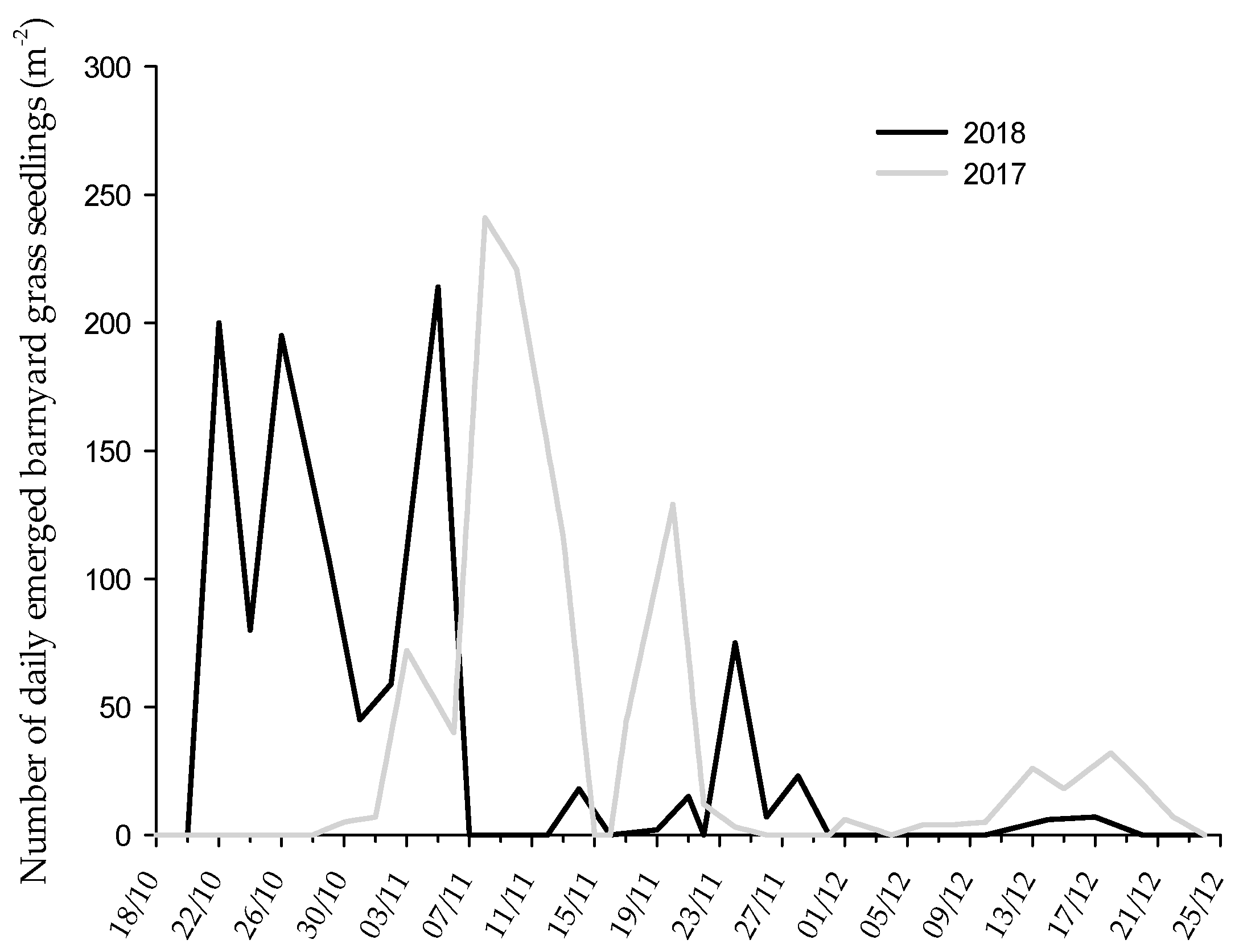
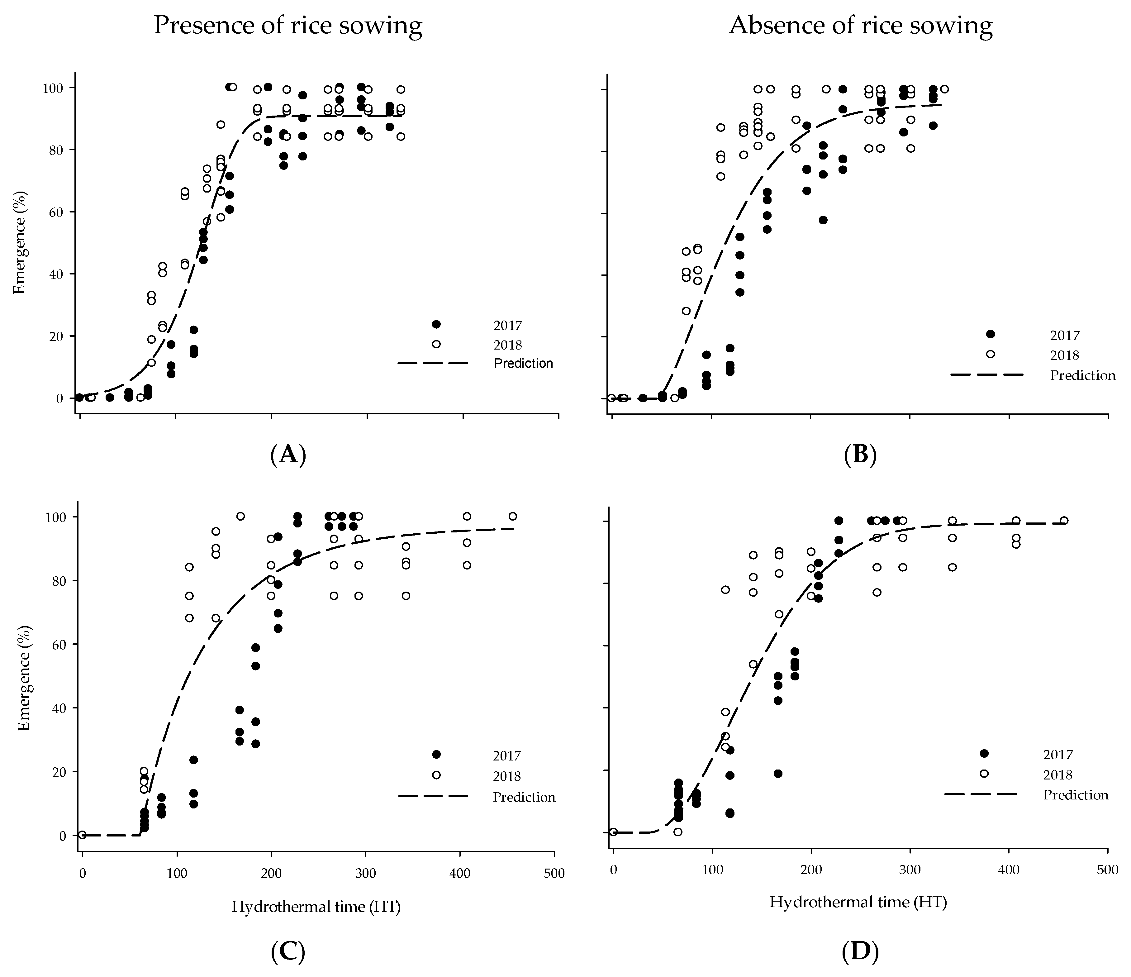
3.1. Barnyard Grass Emergence

The number of emerged barnyard grass seedlings differed between the sowing seasons and cultivation years monitored (Figure 1). However, in the two years, the highest emergence rates of barnyard grass occurred in the first sowing times. These rates were 46.5% and 65.0% higher than those of the second half of November, in 2017 and 2018, respectively.

The years 2017 and 2018 differed considerably in rainfall (data not shown) and soil temperature (Figure 2) at the evaluated months. The year 2018 had colder temperatures in October and at the beginning of December in comparison to the year 2017. However, the month of November was hotter in 2018 than in 2017. The rainfall events occurred during 11 and 13 days for each year, maintaining the soil water potential on better conditions (upper to −0.4 MPa) (data not shown) 56 and 48 days for 2017 and 2018, respectively (Figure 3).

Considering the crop requirement, the accumulated water volume is low. In addition, poor rainfall distribution tends to differentiate the soil water potential (Figure 3). However, in both years, the soil water potential was higher than the base water potential for barnyard grass emergence (−0.95 MPa). Nevertheless, increased accumulations of low-frequency rainfall tend to maintain the water potential for a short period of time, while well-distributed rainfall tended to maintain the soil water potential favorable to weed emergence for longer.

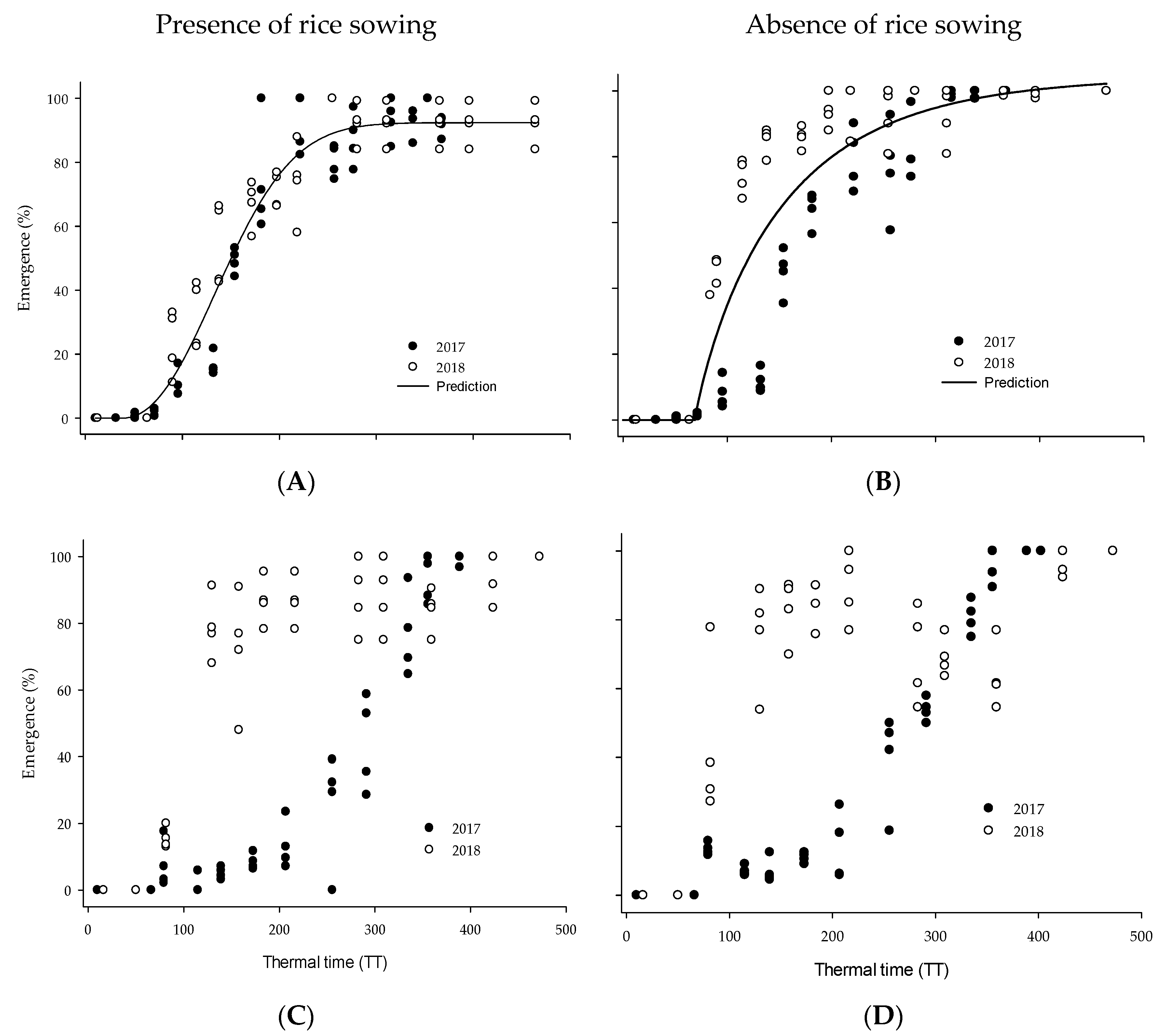
3.2. Thermal and Hidrothermal Time Emergence Models

Using only base temperature parameters (Tb), the model could describe barnyard grass emergence only in the first sowing time (Figure 4;

Table 1. Estimated parameters (a, T50, b, c) of the Weibull function fitted to the thermal time model. (Source: Capão do Leão/RS, 2019).

Mod	a 1		T50		b		c		R 2	p-Value
A2	92.36	±1.7 3	144.50	±3.3	127.16	±26.1	2.22	±0.6	0.95	≤0.0001 *
B	104.44	±7.9	125.79	±8.3	86.02	±15.7	0.88	±0.2	0.85	≤0.0001 *
C	575.08	-	2642.95	-	4417.44	-	0.68	-	0.63	0.9493 ns
D	547.30	-	2681.33	-	4539.96	-	0.67	-	0.62	0.8434 ns

* Significant model; ^ns Nonsignificant model; ¹ “a” is the maximum emergence percentage recorded of Echinochloa sp.; “T₅₀” is the thermal time needed to obtain a 50% emergence; “b” is the rate of increase; “c” is a shape parameter. ² A = Presence of rice sowing on October; B = Absence of rice sowing on October; C = Presence of rice sowing on November; and D = Absence of rice sowing on November. ³ Values represent standard errors.

). However, with the addition of the base water potential (Ψb), the model described barnyard grass emergence in both sowing times (Figure 5;

Table 2. Estimated parameters (a, T50, b, c) of the Weibull function fitted to the hydrothermal time model. (Source: Capão do Leão/RS, 2019).

Mod.	a 1		T50		b		c		R 2	p-Value
A 2	90.34	±2.0 3	115.91	±2.8	128.33	±74.4	3.50	±2.4	0.95	≤0.0001 *
B	95.24	±4.3	110.56	±5.2	83.98	±22.4	1.45	±0.6	0.89	≤0.0001 *
C	96.91	±6.7	109.47	±8.8	71.54	±14.3	0.93	±0.3	0.81	≤0.0001 *
D	99.26	±2.8	140.03	±4.7	127.72	±22.5	1.91	±0.5	0.93	≤0.0001 *

* Significant model; ¹ “a” is the maximum emergence percentage recorded of Echinochloa sp.; “T₅₀” is the thermal time needed to obtain a 50% emergence; “b” is the rate of increase; “c” is a shape parameter. ² A = Presence of rice sowing on October; B = Absence of rice sowing on October; C = Presence of rice sowing on November; and D = Absence of rice sowing on November. ³ Values represent standard errors.

). The precision of the HT model is greater and fits to both seasons as the water potential also influences temperature accumulation and not just Tb. Noteworthy, temperature started to accumulate from sowing in both models.

The emergence model (Weibull function) calculated using climatic data from 2017 and 2018 allows to identify the potential emergence periods of the species for the two sowing times based on HT. Both periods showed a high initial emergence followed by a more gradual emergence pattern (Figure 5). Thus, the cumulative emergence of barnyard grass followed the typical sigmoidal curve, resulting from the normal seedling emergence distribution over hydrothermal time.

4. Discussion

Soil water potential is an important factor that can be measured as a function of barnyard grass emergence. This potential increased right after the rainfall events. Rainfall variability over the years is highly desirable for the development of microclimate models [10]. Therefore, the characteristics of barnyard grass emergence rates, associated with environmental variability, have enabled the development of the thermal time (TT) and hydrothermal time (HT) emergence models.

Studies report different weed emergence rates between sowing times and cultivation years for a range of weed species in different crops such as winter cereals [11], corn, and soybean [3,7]. Notwithstanding, it is difficult to identify the causes of reduction or increase in barnyard grass emergence because several factors may be involved. Among the main factors are the weather conditions during the sowing seasons and cultivation years, soil disturbance, and dormancy conditions, which may have interfered with the emergence and establishment of weeds in the present study. The highest values of daily emergence of barnyard grass tend to occur immediately after rice sowing, with higher emergence rates in the first 10 days. The same was observed with weeds in winter cereals under adequate soil moisture conditions, where 90% of the emergence occurred between 15 and 45 days after sowing [22]. Considering the high barnyard grass soil seed bank in the experimental area, the number of weed seedlings germinating in the different years was not enough to exhaust the soil seed bank, and it is not considered a limiting factor to modeling the barnyard grass emergence.

It is noteworthy that the sowing in October is more prone to continuous barnyard grass emergence, while sowing in November can have more than one emergence of weeds. For southern Brazil conditions, rice sowing in October showed higher barnyard grass emergence than rice sowing in November. The emergence of new crop or weed plants depends on the environmental conditions, which may encourage growth or the capacity for self-thinning in areas with limited resources [23].

The TT model was accurate enough to predict barnyard grass emergence in different regions of the United States of America [12]. However, it is noteworthy that this model is adequate to describe the emergence of barnyard grass and 16 other weed species that emerge in spring and summer when under normal soil moisture conditions [8]. One of the advantages of the TT model over the HT model is that soil temperature parameters are easily accessible, making this type of model practical and useful for farmers [12,24].

Hydrothermal time (HT) models improved the accuracy of the predictions of the thermal time (TT) model in sites with periods of water deficit [25], but their use may extend to some species under adequate soil water availability [8]. The HT model was also more accurate than the TT model for barnyard grass emergence in different regions of Italy [24], and for other species such as Lolium rigidum Gaud. [11] and Conyza bonariensis (L.) Cronq. [26].

The models shows that barnyard grass emergence was higher during early crop development. Some authors report this trend for several weed species, including monocot and dicot species. Such behavior generally guarantees success in the initial establishment and perpetuation of the species [23]. This linear growth occurs mainly in areas of low infestation [27]. During crop development and weed emergence, the establishment or reduction of infestation will depend on environmental conditions and/or the capacity for self-thinning in areas with limited resources and conditions [23].

Thermal and hydrothermal emergence models report Echinochloa crus-galli (L.) Beauv as a species that emerges at intermediate sowing times [5,8], only at relatively low densities (from 6 to 88 m⁻² seedlings), and for a long period in rainfed areas [5]. Nonetheless, lowland areas showed faster barnyard grass emergence. Average infestation was 665.5 and 83.5 m⁻² in the first and second sowing times, at 22 days after sowing, respectively, highlighting these areas. Moreover, this period had different emergence rates. This unevenness in emergence rate is an inherent characteristic of weeds, depending on the types and dormancy conditions of each species [23], in addition to environmental conditions such as light, temperature, and soil moisture.

The emergence model of barnyard grass appears to be robust enough to be used as a tool for weed management. In this study, the model describes the field emergence of barnyard grass not in quantity, but as the emergence ratio during several hydrothermal times. Large areas hinder periodic monitoring; thus, this model enables monitoring weed emergence rate through meteorological information from data collection stations. The parameters of the emergence models can be included in the preparation of spatial maps at the local or regional level using the data available from satellites or meteorological stations. This information can be used to identify conditions and monitor emergence dynamics of barnyard grass and making maps more quickly, which can aid in the decision to spray herbicides with precision, avoiding economic losses. Furthermore, the existing models to predict weed emergence can be used together to assist in the choice of management options [28].

The benefit of using HT instead of TT is due to its capacity to predict emergence pauses caused by low soil moisture, which is important to reduce error in practice, that is, when the emergence model is being applied [7]. In this case, the HT model avoids early applications of herbicides in the field, allowing the best time for weed control. For example, if the farmer decides to control weeds with a postemergence herbicide, it is necessary to wait until the majority of the plants have emerged, without exceeding the control stage. Thereby, the grower may spray the herbicide when cumulative emergence reaches 70 to 80% by assessing weed development stages. Thus, crop modelling, to predict weed emergence, and remote sensing of weeds could be used in a management program. Obviously, no control measures should be taken without inspecting the crop and confirming the presence of weeds.

5. Conclusions

For southern Brazil conditions, the highest emergence rates of barnyard grass occurred in the first sowing time, in October. The hydrothermal time model is suitable for estimating barnyard grass emergence in both sowing times and serves as a tool for decision making on the use of control measures depending on environmental conditions. The thermal time model is suitable for first sowing time only.

References

1. Holst, N.; Rasmussen, I.A.; Bastiaans, L. Field weed population dynamics: A review of model approaches and applications. Weed Res. 2007, 47, 1–14. [Google Scholar] [CrossRef]
2. Masin, R.; Vasileiadis, V.P.; Loddo, D.; Otto, S.; Zanin, G. A single-time survey method to predict the daily weed density for weed control decision-making. Weed Sci. 2011, 59, 270–275. [Google Scholar] [CrossRef]
3. Zandoná, R.R.; Agostinetto, D.; Ruchel, Q. Modelagem matemática do fluxo de emergência de plantas daninhas: Ferramenta para decisão no manejo de cultivos. Rev. Bras. Herb. 2018, 17, 3–11. [Google Scholar]
4. Loddo, D.; Farshid, G.F.; Zahra, R.; Roberta, M. Base temperatures for germination of selected weed species in Iran. Plant Prot. Sci. 2017, 54, 60–66. [Google Scholar]
5. Dorado, J.; Sousa, E.; Calha, I.M.; González-Andújar, J.L.; Fernández-Quintanilla, C. Predicting weed emergence in maize crops under two contrasting climatic conditions. Weed Res. 2009, 49, 251–260. [Google Scholar] [CrossRef]
6. Masin, R.; Loddo, D.; Benvenuti, S.; Otto, S.; Zanin, G. Modeling weed emergence in Italian maize fields. Weed Sci. 2012, 60, 254–259. [Google Scholar] [CrossRef] [Green Version]
7. Masin, R.; Loddo, D.; Gasparini, V.; Otto, S.; Zanin, G. Evaluation of weed emergence model AlertInf for maize in soybean. Weed Sci. 2014, 62, 360–369. [Google Scholar] [CrossRef]
8. Werle, R.; Sandell, L.D.; Buhler, D.D.; Hartzler, R.G.; Lindquist, J.L. Predicting emergence of 23 summer annual weed species. Weed Sci. 2014, 62, 267–279. [Google Scholar] [CrossRef]
9. Royo-Esnal, A.; Torra, J.; Conesa, J.A.; Forcella, F.; Recasens, J. Modeling the emergence of three arable bedstraw (Galium) species. Weed Sci. 2010, 58, 10–15. [Google Scholar] [CrossRef]
10. Royo-Esnal, A.; Necajeva, J.; Torra, J.; Recasens, J.; Gesch, R.W. Emergence of field pennycress (Thlaspi arvense L.): Comparison of two accessions and modelling. Ind. Crop. Prod. 2015, 66, 161–169. [Google Scholar] [CrossRef] [Green Version]
11. Izquierdo, J.; Bastida, F.; Lezaún, J.M.; Del Arco, M.J.S.; Gonzalez-Andujar, J.L. Development and evaluation of a model for predicting Lolium rigidum emergence in winter cereal crops in the Mediterranean area. Weed Res. 2013, 53, 269–278. [Google Scholar] [CrossRef]
12. Lundy, M.E.; Hill, J.E.; Van Kessel, C.; Owen, D.A.; Pedroso, R.M.; Boddy, L.G.; Fischer, A.J.; Linquist, B.A. Site-specific, real-time temperatures improve the accuracy of weed emergence predictions in direct-seeded rice systems. Agric. Syst. 2014, 123, 12–21. [Google Scholar] [CrossRef]
13. de Lima Fruet, B.; Merotto, A.; da Rosa Ulguim, A. Survey of rice weed management and public and private consultant characteristics in Southern Brazil. Weed Tech. 2020, 34, 351–356. [Google Scholar] [CrossRef]
14. Heap, I. International Survey of Herbicide Resistant Weeds. Available online: http://www.weedscience.org/ (accessed on 14 May 2020).
15. Zoneamento Agrícola de Risco Climático. Available online: http://www.agricultura.gov.br/assuntos/riscos-seguro/risco-agropecuario/zoneamento-agricola (accessed on 17 June 2017).
16. Counce, P.A.; Keisling, T.C.; Mitchell, A.J. A uniform, objective, and adaptative system for expressing rice development. Crop Sci. 2000, 40, 436–443. [Google Scholar] [CrossRef] [Green Version]
17. Lorenzi, H. Manual de Identificação e Controle de Plantas Daninhas Plantio Direto e Convencional, 7th ed.; Plantarum: Nova Odessa, Brazil, 2014; p. 384. [Google Scholar]
18. Concenço, G.; Parfitt, J.M.B.; Downing, K.; Larue, J.; Silva, J.T. Rice development and water demand under drought stress imposed at distinct growth stages. Afr. J. Agric. Res. 2016, 11, 4147–4156. [Google Scholar]
19. Gummerson, R.J. The effect of constant temperatures and osmotic potential on the germination of sugar beet. J. Exp. Bot. 1986, 37, 729–741. [Google Scholar] [CrossRef]
20. Chantre, G.R.; Blanco, A.M.; Lodovichi, M.V.; Bandoni, A.J.; Sabbatini, M.R.; López, R.L.; Vigna, M.R.; Gigón, R. Modeling Avena fatua seedling emergence dynamics: An artificial neural network approach. Comp. Electro. Agric. 2012, 88, 95–102. [Google Scholar] [CrossRef]
21. Roman, E.S.; Murphy, S.D.; Swanton, C.J. Simulation of Chenopodium album seedling emergence. Weed Sci. 2000, 48, 217–224. [Google Scholar] [CrossRef]
22. Fernandez-Quintanilla, C.; Barroso, J.; Recasens, J.; Sans, X.; Torner, C.; Sanchez Del Arco, M.J. Demography of Lolium rigidum in winter barley crops: Analysis of recruitment, survival and reproduction. Weed Res. 2000, 40, 281–291. [Google Scholar] [CrossRef]
23. Radosevich, S.R.; Holt, J.S.; Ghersa, C.M. Ecology of Weeds and Invasive Plants: Relationship to Agriculture and Natural Resource Management, 3rd ed.; Wiley-Interscience: Hoboken, NJ, USA, 2007; p. 400. [Google Scholar]
24. Masin, R.; Loddo, D.; Benvenuti, S.; Zuin, M.C.; Macchia, M.; Zanin, G. Temperature and water potential as parameters for modeling weed emergence in central-northern Italy. Weed Sci. 2010, 58, 216–222. [Google Scholar] [CrossRef]
25. Leguizamon, E.S.; Fernandez-Quintanilla, C.; Barroso, J.; Gonzalez-Andujar, J.L. Using thermal and hydrothermal time to model seedling emergence of Avena sterilis ssp. ludoviciana in Spain. Weed Res. 2005, 45, 149–156. [Google Scholar] [CrossRef]
26. Zambrano-Navea, C.; Bastida, F.; Gonzalez-Andujar, J.L. A hydrothermal seedling emergence model for Conyza bonariensis. Weed Res. 2013, 53, 213–220. [Google Scholar] [CrossRef] [Green Version]
27. Silva, A.F.; Concenço, G.; Aspiazú, I.; Ferreira, E.A.; Galon, L.; Coelho, A.T.C.P.; Silva, A.A.; Ferreira, F.A. Interferência de plantas daninhas em diferentes densidades no crescimento da soja. Planta Daninha. 2009, 27, 75–84. [Google Scholar] [CrossRef] [Green Version]
28. Boddy, L.G.; Bradford, K.J.; Fixcher, A.J. Population based threshold models describe weed germination and emergence patterns across varying temperature, moisture and oxygen conditions. J. Appl. Ecol. 2012, 49, 1225–1236. [Google Scholar] [CrossRef]
Figure 1. Distribution of the number of daily emerged Echinochloa sp. seedlings over the two growing seasons, 2017/2018 and 2018/2019. (Source: Capão do Leão/RS, 2019).
Agronomy 10 01756 g001
Figure 2. Soil temperature data observed in the experimental area during the experiment. (Source: Capão do Leão/RS, 2019).
Agronomy 10 01756 g002
Figure 3. Daily soil water potential (MPa) observed in the experimental area during the experiment: Continuous and dotted lines refer to the water potential of 2017 and 2018, respectively. (Source: Capão do Leão/RS, 2019).
Agronomy 10 01756 g003
Figure 4. Thermal time model for Echinochloa sp. emergence at different sowing times ((A,B)—October; (C,D)—November) in Capão do Leão city, Rio Grande do Sul State, at the 2017/18 and 2018/19 growing seasons. Lines represent the predicted emergence; symbols represent the observed emergence. (Source: Capão do Leão/RS, 2019).
Agronomy 10 01756 g004
Figure 5. Hydrothermal time model for Echinochloa sp. emergence at different sowing times ((A,B)—October; (C,D)—November) in Capão do Leão city, Rio Grande do Sul State, at the 2017/18 and 2018/19 growing seasons. Lines represent the predicted emergence; symbols represent the observed emergence. (Source: Capão do Leão/RS, 2019).
Agronomy 10 01756 g005