Assessment of the Use of Geographically Weighted Regression for Analysis of Large On-Farm Experiments and Implications for Practical Application

Abstract

On-farm experimentation (OFE) is a farmer-centric process that can enhance the adoption of digital agriculture technologies and improve farm profitability and sustainability. Farmers work with consultants or researchers to design and implement experiments using their own machinery to test management practices at the field or farm scale. Analysis of data from OFE is challenging because of the large spatial variation influenced by spatial autocorrelation that is not due to the treatment being tested and is often much larger than treatment effects. In addition, the relationship between treatment and yield response may also vary spatially. We investigate the use of geographically weighted regression (GWR) for analysis of data from large on-farm experiments. GWR estimates local regressions, where data are weighted by distance from the site using a distance-decay kernel. It is a simple approach that can be easily explained to farmers and their agronomic advisors. We use simulated data to test the ability of GWR to separate yield variation due to treatment from any underlying spatial variation in yield that is not due to treatment; show that GWR kernel bandwidth can be based on experimental design to accurately separate the underlying spatial variability from treatment effects; and demonstrate a step-wise model selection approach to determine when the response to treatment is global across the experiment or locally varying. We demonstrate our recommended approach on two large-scale experiments conducted on farms in Western Australia to investigate grain yield response to potassium fertiliser. We discuss the implications of our results for routine practical application to OFE and conclude that GWR has potential for wide application in a semi-automated manner to analyse OFE data, improve farm decision-making, and enhance the adoption of digital technologies.

1. Introduction

Precision agriculture (PA) uses data from multiple sources to map and analyse yield variability and manage crops accordingly [1]. It has recently been defined as follows: precision agriculture is a management strategy that gathers, processes, and analyses temporal, spatial, and individual data and combines it with other information to support management decisions according to the estimated variability for improved resource use efficiency, productivity, quality, profitability, and sustainability of agricultural production [2]. While PA was originally thought to have great potential [3], its uptake has been lower than anticipated [4,5]. A recent study of the Australian grains sector found that while 87% of survey respondents had access to a yield monitor, only 57% of those generate yield maps and only 62% of grain growers who generate yield maps use them to delineate management zones. Thus, “in spite of typically having yield maps for 5–7 years, 38% of growers have not made use of them for decision-making relating to targeting management” [6]. One possible cause of this lack of adoption is the need for specialised consultants and software [1]. The development of software and decision support systems for PA has been slow [5] and requires a systems approach that encompasses databases, novel analytical techniques, and mechanisms for farmers to access information and advice [7] as well as “big data” methodologies [8]. Even as PA software becomes more widely available, uptake also depends on the development of protocols, economic assessment of performance, and the perceptions of potential adopters [9]. Other factors include the relative advantage (over previous practices) and trialability [10]. While being largely driven by the desire to increase profitability, PA adoption is also influenced by education, perceived ease of use, and access to expert consultants and contractors [11,12], which “initiates a learning process, enabling potential users to become more aware and confident about PA tools” [13].

On-farm experimentation (OFE) has been proposed as a process to enhance the adoption of digital technologies in agriculture, develop farmer competence, and improve profitability [14,15,16], and it is becoming widespread [17,18]. OFE is farmer-centric, where farmers work with consultants and/or researchers to design and implement large-scale experiments on their farms to test management practices. By enabling trialability within a co-learning framework, OFE has the potential to overcome multiple existing barriers to PA adoption. However, the development of software and methods of analysis for data from OFE is still required.

Similar to PA, OFE is enabled by digital agriculture technology including the automated steering of farm machinery, programmable variable rate applicators, and yield monitors. Farmers use their own machinery to conduct large field-scale experiments. The results of experiments usually take the form of geographically referenced yield data recorded by yield monitors that are standard in most modern harvesting machinery. Data recorded by other types of sensors mounted on machinery, satellites, or drones may also be used; for example, measures of greenness such as the normalised difference vegetation index (NDVI) or protein measurements. However, because the same methods of analysis can be applied to any continuous measurement, we discuss yield measurements from hereon. Experiments might compare discrete treatments such as the variety [19] or types of soil amelioration, quantify response to different rates of a single treatment such as fertiliser or fungicide [16,20,21], or consider multiple treatments. Various designs are used, including strip trials [22,23,24,25,26,27], nitrogen-rich strips [28], and checkerboards [29,30].

Agronomic experiments have historically been performed by researchers using small plot sizes and principles of experimental design so that effects of treatments can be analysed while minimising environmental effects [31,32]. However, results from small-scale experiments do not transfer well to on-farm practice where there is massive spatial and temporal variability in crop yields, and environmental causes of variation are either unknown or uncontrollable [33]. Furthermore, many farmers find insights from formal experimentation difficult to apply in practice [14]. In contrast, OFE is conducted at the scale at which management decisions are made, using the same machinery, with experimentation as the core of a continuous learning process that provides insight to the farmer. The farmer learns to perceive value in data collected on the farm and uses it to modify management to support PA or other management decisions.

With increasing opportunity and uptake of variable rate controllers to install OFE, benefits beyond the enhancement of PA adoption become evident. Being both larger and simpler to implement than traditional plot experiments, OFE can be conducted at more locations, thereby providing more relevant information about effects of treatments at those locations and facilitating a meta-analysis of results from many experiments [19]. Since on-farm experiments can be implemented cheaply, OFE is a cost-effective technique that can also contribute new knowledge to agricultural research.

Analysis of data from OFE is challenging because of large spatial variation in yield that:

• is influenced by spatial auto-autocorrelation;
• is not due to the treatment being tested [34]; and
• is often much larger than the variation due to treatment effects.

Spatial auto-correlation occurs when Tobler’s First Law applies: “Everything is related to everything else. But near things are more related than distant things.” [35]. Thus, spatial data are typically not independent, and regression models that assume independence cannot be applied. Various methods have been used to handle spatial autocorrelation in large-scale agricultural experiments. For experiments without geo-referenced measurements, these include standard methods typically applied to small plot experiments, such as experimental design with blocking, global regressions that allow spatially autocorrelated error terms [36], and linear mixed models [19,33,34,37,38]. However, standard methods are frequently not suitable for the analysis of on-farm experiments that are conducted using large plots in simple designs that may be systematic rather than randomised, and where there are multiple geo-referenced measurements recorded for each plot.

Spatial regression [39,40,41] and Bayesian conditional auto-regressive models [42] have been used to account for spatial autocorrelation in OFE data. However, these methods assume a global relationship between treatment and yield, and in large experiments, the relationship between treatment and yield may vary spatially. Lark and Wheeler [43] estimated local nitrogen response curves using moving window regression with a spatial error model. Pringle et al. [44] used co-kriging to interpolate response from all levels of a variable input onto a common grid, producing a yield corresponding to each level at each cell in the grid. For each cell, they then fit local polynomial response curves. Co-kriged yield from variable and discrete inputs has also been used for point-wise hypothesis testing, effectively considering fertiliser rates to be discrete treatments rather than estimating response curves directly [45,46]. In addition, more simple comparisons of two treatment types laid in strips have been performed using local methods [22,47] and an examination of changes across plot boundaries has also been considered [20].

Geographically weighted regression (GWR) is an alternative and simpler approach that has recently been used to estimate spatially varying response curves from OFE [48,49]. GWR can be simply described as performing local linear regressions, where data are weighted by distance from each local site [50,51,52]. The ability to describe GWR so simply is a major advantage of GWR, meaning that it can be easily explained to farmers and their agronomic advisors and it has the potential to be applied in a semi-automated or automated way in computer software. Consider the example of an on-farm experiment that aims to detect the response of yield to different fertiliser rates. Fertiliser response typically increases up to a maximum yield before reaching a plateau or decreasing as more fertiliser is applied [53]. It is often modelled using linear-plateau [54], quadratic-plateau [55], linear plus exponential [56], or modified Mitscherlich [57] functions. If the experiment applies rates in the approximately linear part of the fertiliser response curve, basic linear GWR can be used to estimate and map the spatially varying intercepts and slopes. The intercept map will capture spatial variation in yield that is not due to the applied fertiliser, and the slope map will capture the local yield response to fertiliser. We expect data analysis using GWR to be part of a broader OFE process of co-learning. For that process to lead to practice change, the results of analysis must be assimilated with a farmer’s prior knowledge and intuition. The outputs from GWR using linear regressions are ideal for this, as they can be visualised using two simple maps of intercept and response that are easily understood and contextualised by farmers. They allow farmers to visualise spatial variation in yield and in response to fertiliser and adjust management practices using data in conjunction with their experience and intuition. This added interpretation of the analysis encourages and enables farmers to use data and evidence-based decision-making as an operational part of farm management. Making OFE a routine part of farming will bridge the disconnect between farmers and researchers, allowing for the continuous learning and improvement in farm management as well as generating new knowledge in the agricultural domain.

While local linear regressions cannot be used to determine yield-maximising or profit-maximising rates of fertiliser, OFE can have several objectives depending on the interests of the experimenter. The optimisation of inputs may not be the prime objective. In the case where we investigate using local linear regressions, the primary goal of the experiment is to quantify the relationship between applied fertiliser and yield and how that relationship varies in space. Additional learning can also arise from considering causes of variation in non-treatment effects captured by the intercept, which can offer insight into pre-existing soil nutrient supplies or causes of yield variability that may be due to soil constraints, weeds, or disease [14]. “One difficulty with GWR is that the estimated parameters are, in part, functions of the weighting function or kernel selected in the method” [50]. GWR results crucially depend on the kernel bandwidth, which determines the rate at which weights decay so that larger bandwidths lead to smoother changes in model parameters. Bandwidth is usually selected by minimising the leave-one-out cross-validation error or measuring that balance accuracy with model complexity such as the Akaike Information Criterion (AIC) [58] or the corrected AIC (Amick) [52,59]; see Section 2.3.2. However, because OFE data are densely distributed in space and have a non-random structure due to experimental design, these standard approaches to bandwidth selection can result in over-fitted models and confounded estimates of spatial and treatment effects. Rakshit et al. [48] describe and demonstrate two approaches to bandwidth selection that can be used for OFE: bandwidth based on the experimental design and spatial k-fold cross-validation [60].

An important question for potential practitioners of PA is whether parts of a paddock respond differently to treatment and should therefore be managed differently [43]. This is an issue of model selection: is the relationship between treatment and yield global, or are locally varying models required? Two categories of on-farm experiments can be defined: (1) those that aim to estimate local response curves for a variable input assuming that they vary spatially across a field, and (2) those that assess response globally across a field [34]. One approach for exploring non-stationarity in treatment–yield relationships is to apply standard methods to predefined landscape zones [40]. This can be also be considered in a geostatistical framework by comparing the use of global or local semivariograms. Pringle, McBratney, and Cook [44] compared global and local kriging methods by the use of an evaluation set containing 10% of the data from two field experiments that were systematic in design. They concluded that a local model was only justified for one of the two experiments, and the other could therefore be addressed as a whole. Model selection for GWR is commonly performed by comparing GWR with ordinary least squares regression applied to the entire dataset. Since yield data from OFE have large, spatially auto-correlated non-treatment effects, we suggest comparing GWR with “mixed” GWR, where the model intercept can vary spatially to capture spatial variation in yield, but the slope of the regression, or response, is fixed globally. GWR and mixed GWR models can be compared using the AICc, and the significance testing of terms is also possible [61,62].

The objective of this study is to assess whether GWR can be used to estimate spatially varying differences in fertiliser response within the approximately linear part of fertiliser response curves for use in the broader OFE process of co-learning and data-driven decision-making. While we are aware that by considering only the linear part of the response curve, we cannot determine yield-maximising or profit-maximising rates of fertiliser, we are primarily interested in assessing the use of GWR for quantifying the relationship between applied fertiliser and yield, and determining if and how that relationship varies in space. We do this by simulating on-farm experiments with linear response to fertiliser treatment and using the simulated data to assess the ability of GWR to separate treatment effects from non-treatment effects. We consider two issues of importance in the application of GWR to OFE: (1) bandwidth selection and (2) model selection to determine whether the relationship between treatment and yield is global or spatially varying. We test the use of a bandwidth based on experimental design and show that it provides a better separation of non-treatment and treatment effects and a more accurate estimation of treatment effects than the usual approach of minimising the AICc. We also propose and demonstrate a stepwise model selection approach for determining whether a global or local model of treatment effects should be used.

The article is structured as follows. Materials and methods are outlined in Section 2. Section 2.1 describes the simulated data that we use to test the ability of GWR to accurately separate underlying spatial variation in yield that is not due to treatment from treatment effects and to assess methods for bandwidth selection and model selection. Section 2.2 describes two on-farm experiments undertaken in Western Australia on which we demonstrate the application of GWR to understand spatial variation in yield response to potassium fertiliser. The GWR method is described in detail in Section 2.3. Results are presented in Section 3. Section 3.1 contains the results using simulated data and subsequent recommendations for application of GWR to OFE in practice. Section 3.2 applies these recommendations to the analysis of the two potassium trials. Finally, we discuss our results and implications for the practical application of GWR for the analysis of OFE in computer software systems and decision tools.

We used the ‘GWmodel’ R package [63,64] to conduct this research and provide R code as Supplementary Materials. Some modifications to the GWmodel package have been made to speed up the estimation of mixed GWR models, and they are freely available from https://github.com/fionahevans/GWmodelFE.

2. Materials and Methods

2.1. Simulated Data

Data are simulated for three likely scenarios:

• Global linear response to fertiliser
• Linear response to fertiliser that varies within spatial zones
• Locally varying linear response to fertiliser

For each scenario, minimum yield ($yield.min$), the yield when no fertiliser is applied, is assumed to vary spatially. It is simulated as a spatially autocorrelated random field with mean 2500 kg ha⁻¹, using an exponential variogram with sill equal to 2500 × 10² and range equal to 30 pixels. A fertiliser strip trial is simulated using a randomised complete block design with four rates (0, 30, 60, and 100) and two repetitions. Each strip is 3 pixels (30 m) wide. The response to fertiliser is added to the minimum yield.

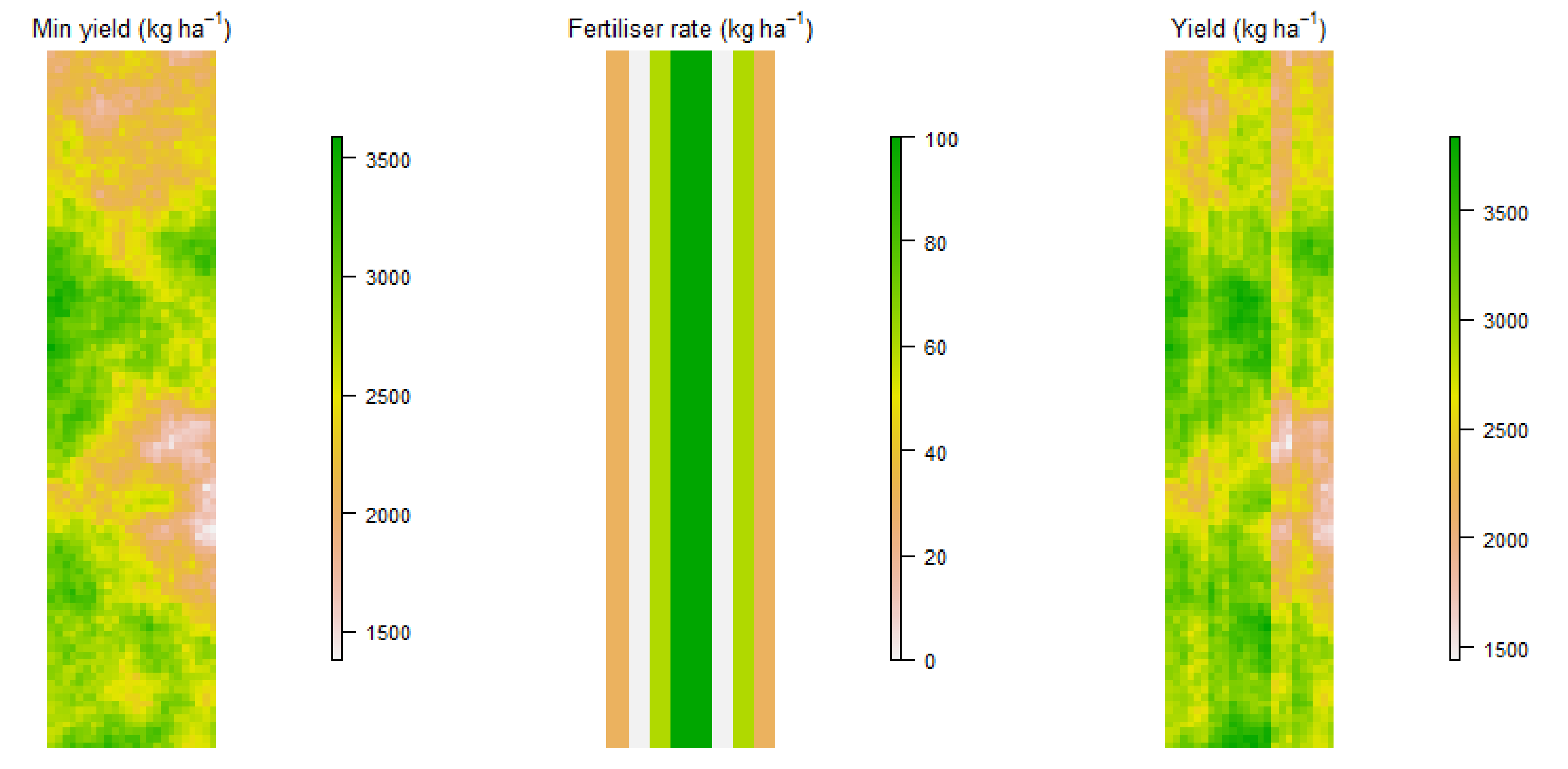
2.1.1. Global Linear Response to Fertiliser

The effect of fertiliser is simulated globally as:

$$yield=yield.min + 6 \ast rate.$$

where $rate$ is the amount of fertiliser applied in kg ha⁻¹. The coefficient 6 corresponds to a global response of 6 kg of yield per kilogram of fertiliser applied. The simulated experiment, comprised of $yield.min$, $rate$, and $yield$, is shown in Figure 1.

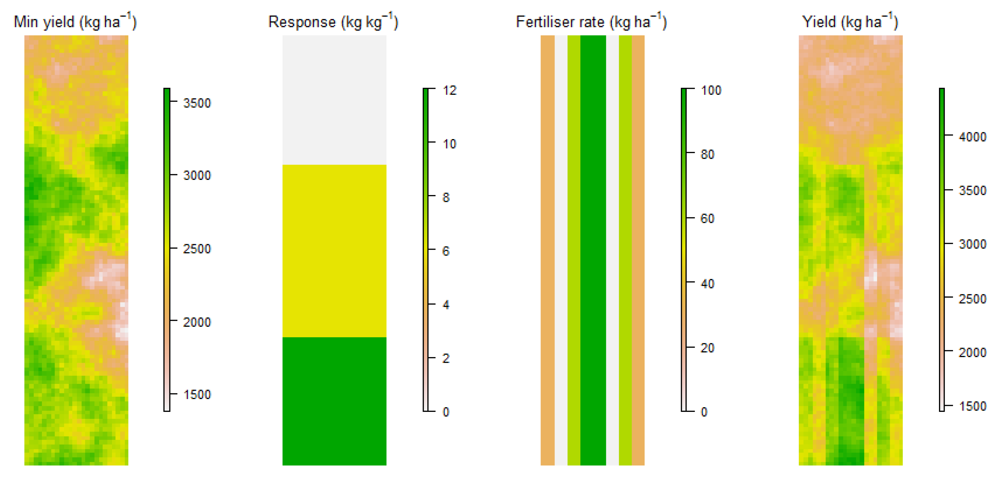
2.1.2. Linear Response to Fertiliser that Varies within Spatial Zones

Local linear response is assumed to vary across three spatial zones, where the northern zone has no response, the middle zone has the same response as for the global linear simulation, and the southern zone has twice the response of the global linear simulation. The simulated experiment, comprised of $yield.min$, zone $\mathrm{response}$, fertiliser $rate$, and $yield$, is shown in Figure 2.

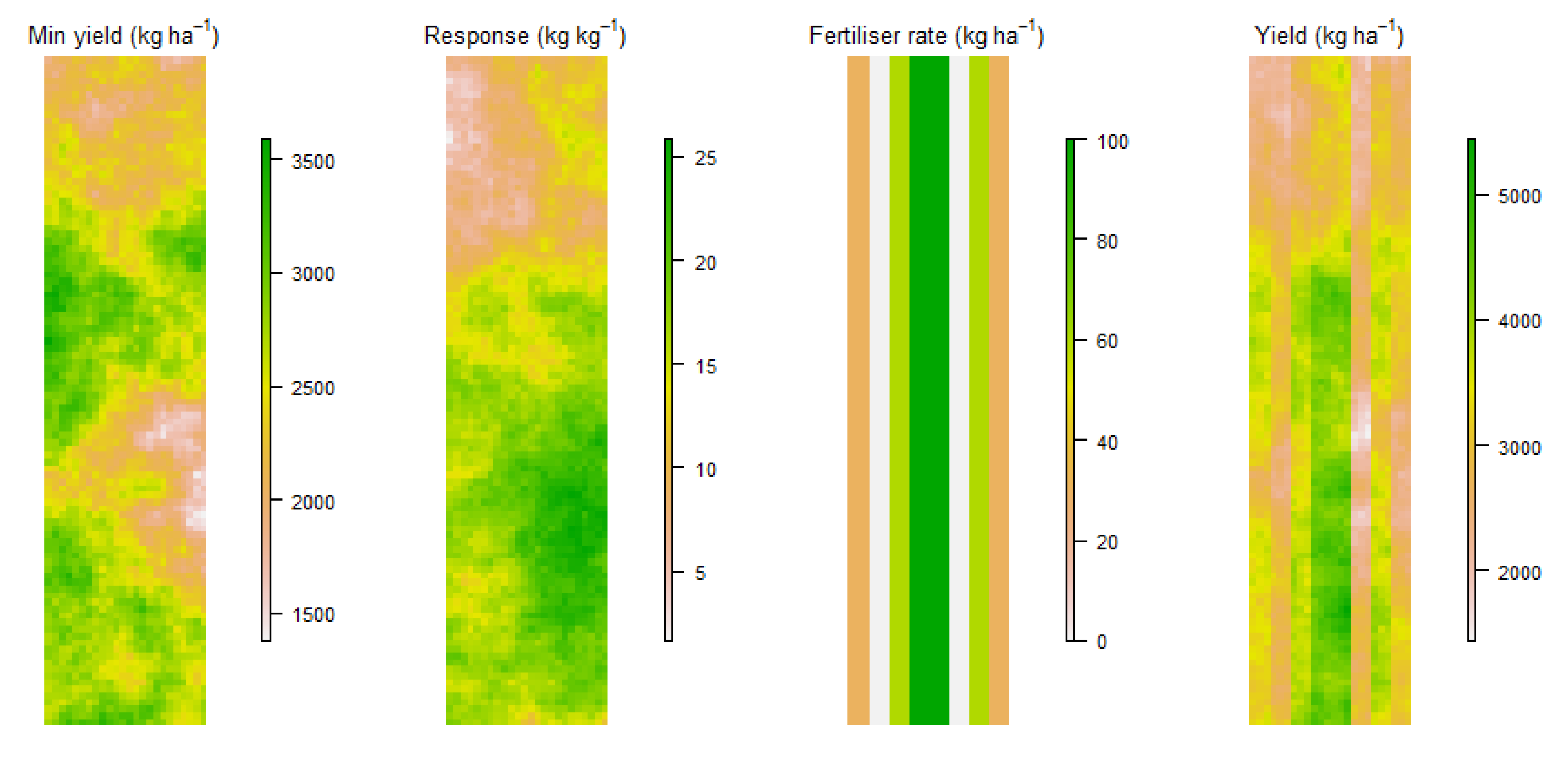
2.1.3. Locally Varying Linear Response to Fertiliser

The effect of fertiliser is simulated locally as:

$$yield=yield.min+response\ast rate.$$

where $\mathrm{response}$ is simulated as a spatially autocorrelated random field with mean 6 (the coefficient used to simulate global linear response), using an exponential variogram with sill = 60 and range = 100. Local response to treatment varies at a larger scale than other yield variation. The simulated experiment, comprised of $yield.min$, $\mathrm{response}$, $rate$, and $yield$, is shown in Figure 3.

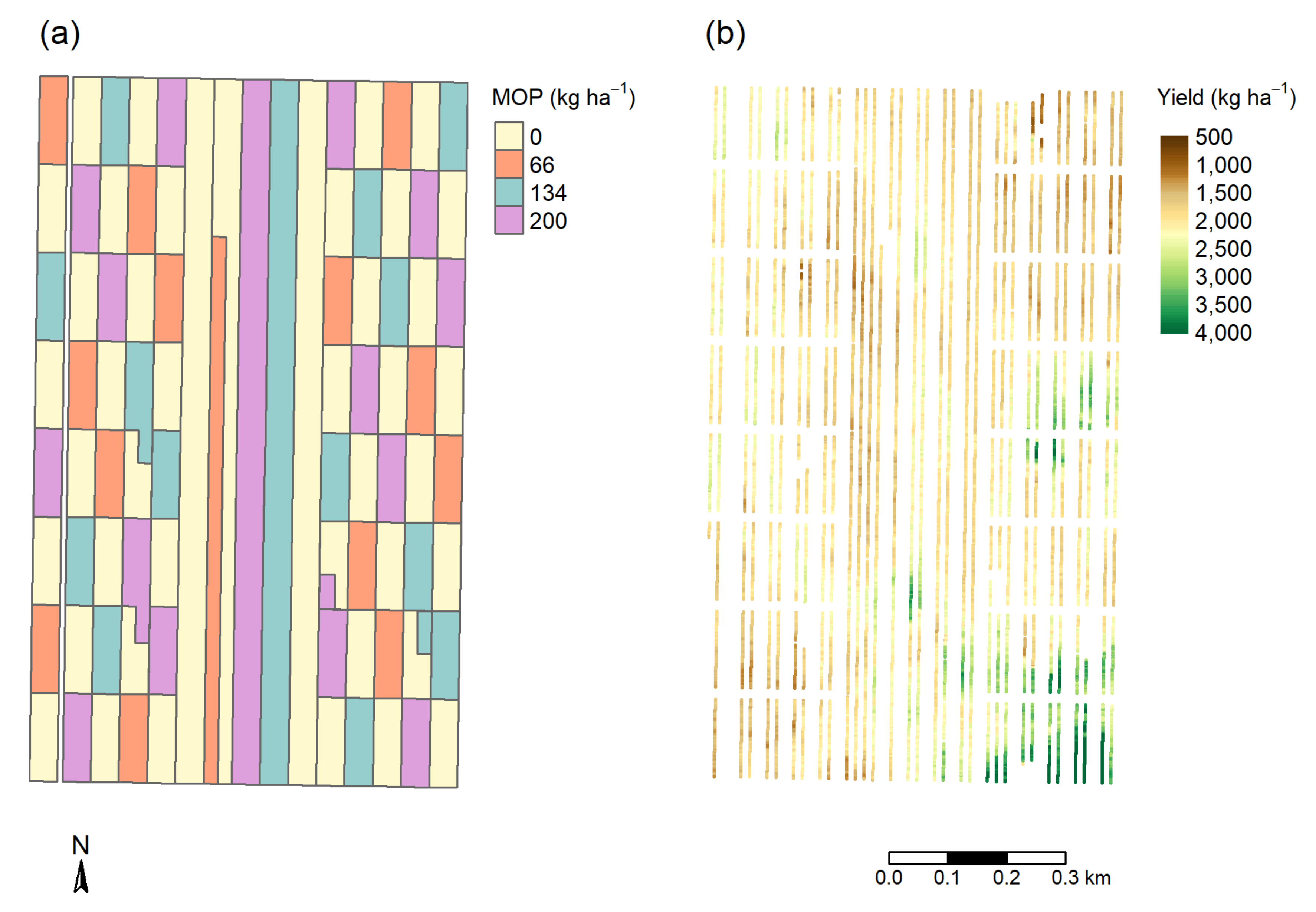
2.2. Potassium Trials

Two large-scale experiments were conducted on farms in the grainbelt of Western Australia to investigate grain yield response to potassium fertiliser Muriate of Potash (MOP, or potassium chloride, KCl, 50% potassium).

2.2.1. Cunderdin Trial

An on-farm experiment was conducted near Cunderdin (31.68 S, 117.17 E), approximately 150 km east of Perth, to investigate barley yield response to potassium in 2018. Four rates of MOP were applied, with two repetitions, using a randomised complete block design in a strip trial (Figure 4). The strips were 12 m wide and approximately 900 m long. Yield monitor data were collected using a harvester with 12 m swath width and cleaned to remove:

• Extreme high and low yields.
• Extreme high and low harvester speeds.

2.2.2. Narambeen Trial

An on-farm experiment was conducted near Narambeen (32.11° S, 118.67° E) to investigate wheat yield response to potassium in 2019. Four rates of MOP were applied in a trial design comprised of both strips and a checkerboard design (Figure 5). The strips were approximately 30 m wide and 1200 m long. In the checkerboard, each strip was split into eight plots approximately 150 m in length. Some errors in fertiliser placement occurred, and therefore, the trial design was altered post hoc to adjust some plot boundaries. Yield monitor data were collected using a harvester with 15 m swath width and cleaned using the protocol above to remove locations near the boundaries of experimental plots where there was a possibility of mixed treatments.

2.3. Geographically Weighted Regression (GWR)

2.3.1. Basic GWR

In its simplest form, GWR performs local linear regressions, accounting for spatial auto-correlation by weighting data by distance from each local site using a distance–decay kernel [50,51,52]. More generally, GWR performs local likelihood estimation [59,65], which means that a wider range of local template models can be used (such as generalised linear models), hypothesis testing can be performed using local t-scores, and models can be compared using model selection criteria.

Consider spatial data collected at geographic locations $\left(u_i,v_i\right)$ for $i=1,\dots ,n$. Let y be the response variable and $X=\left(x_1,\dots ,x_m\right)$ be the explanatory variables. The basic GWR model takes the form

$$y_i={\beta }_0\left(u_i,v_i\right)+{\displaystyle \sum }_{k=1}^m{\beta }_k\left(u_i,v_i\right)x_{ik}+{ϵ}_i$$

(1)

where ${\beta }_0\left(u_i,v_i\right)$ and ${\beta }_k\left(u_i,v_i\right)$ are the coefficients of the local regression at the i-th location and ${ϵ}_i$ is the error. Letting $\beta =\left({\beta }_0,\dots ,{\beta }_k\right)$, the maximum likelihood estimator for the i-th location is given by

$${\widehat{\beta }}_i={\left(X^T{W}_{i}X\right)}^{-1}{X}^T{W}_{i}y=C_{i}y$$

(2)

where $W_i$ is an n by n diagonal matrix whose diagonal elements correspond to the weights based on distance from the i-th data point used in the local regression and $C_i={\left(X^T{W}_{i}X\right)}^{-1}{X}^T{W}_i$. The variance of the estimated parameters is given by

$$\mathrm{Var}\left[\widehat{{\beta }_i}\right]={\sigma }^2{C}_i{C}_i^T$$

(3)

where ${\sigma }^2$ is the normalised residual sum of squares from the local regression. The hatmatrix $S$ is defined to be the matrix with $n$ rows given by $X_i{C}_i$. Writing ${\nu }_1=tr\left(S\right)$ and ${\mathsf{\nu }}_2=\mathrm{tr}\left(S^{T}S\right)$, the effective degrees of freedom is given by ${\gamma }^{\ast }=n-2{\nu }_1+{\nu }_2$, and ${\sigma }^2$ is given by

$${\sigma }^2=\frac{1}{{\gamma }^{\ast }}{\displaystyle \sum }_{i=1}^n{\left(y_i-\widehat{y_i}\right)}^2$$

(4)

and the local t-score for the j-th explanatory variable can be defined as

$$t_j\left(u_i,v_i\right)=\frac{{\widehat{\beta }}_j\left(u_i,v_i\right)}{\widehat{\sigma \sqrt{s_{jj}}}}$$

(5)

where $s_{jj}$ is the j-th diagonal entry in $S{S}^T$. A formal hypothesis test is performed using the corresponding p-value with $\mathsf{\gamma }$ degrees of freedom. To avoid false positives due to multiple testing, p-values can be adjusted using various methods [66]. Note that these p-values test whether local regression coefficients are significant (i.e., whether there is a yield response to treatment) but do not test the stationarity of covariates (i.e., whether yield response to treatment should be modelled as a global locally varying).

2.3.2. Bandwidth Selection for GWR

Comparison of kernels and bandwidth selection are usually performed using model selection criteria that encode a trade-off between the accuracy of the model and its complexity, such as the AIC [58] or the corrected AIC (AICc) recommended for GWR [52,59]. The AICc is given by:

$$AICc=2n\mathit{log}\left({\sigma }^2\right)+n\mathit{log}2\pi +n\left\{\frac{n+tr\left(S\right)}{n-2-tr\left(S\right)}\right\}$$

(6)

where the hatmatrix S, defined in Section 2.3.1 is a function of the bandwidth. The AICc is composed of two parts: the first is the negative of the log-likelihood or model accuracy, and the second is a measure of the number of parameters or model complexity. A good model is one that maximises accuracy while minimising complexity; thus, smaller values of the AICc indicate better models.

The AIC is asymptotically equivalent to leave-one-out cross-validation [67], which means that it can provide overly generous estimates of model accuracy for large datasets. Since OFE data are large, densely distributed in space, and have a non-random structure due to experimental design, bandwidth selection using AICc can result in over-fitted models and confounded estimates of spatial and treatment effects. A recently proposed method for selecting bandwidth is based on the experimental design used, so that local regressions capture data covering the full range of treatments [48]. The recommended bandwidth is $\left(\tau -1\right)d/2$, where d is the distance between adjacent treatments or the width of the strips in the trial, and $\tau$ is the number of treatments. In some cases, this may not be large enough to accommodate all treatments for some local regressions, in which case a larger bandwidth should be used.

We compare bandwidth selection by minimising AICc with bandwidth selection based on strip widths and experimental design.

2.3.3. Mixed GWR and Model Selection

Basic GWR assumes that all regression coefficients vary geographically. In some situations, this may not be the case; for example, yield response to fertiliser application may be constant across a trial. In this case, a mixed GWR model that allows some coefficients to be global may better describe the data. The mixed GWR model has the form

$$y_i={\beta }_0\left(u_i,v_i\right)+{\displaystyle \sum }_{k=1}^q{\beta }_k{x}_{ik}+{\displaystyle \sum }_{k=q+1}^m{\beta }_k\left(u_i,v_i\right)x_{ik}+{ϵ}_i$$

(7)

where $X_a=\left(x_1,\dots ,x_q\right)$ are response variables with fixed or global coefficients and $X_b=\left(x_{q+1},\dots ,x_m\right)$ are response variables with spatially varying coefficients.

The estimation of mixed GWR models is performed as follows [52]:

• For each column of $X_a$,

  i.

  Regress the column against $X_b$ using basic GWR.

  ii.

  Compute the residual from the above regression.

• Regress y against $X_b$ using basic GWR.
• Compute the residual from the above regression.
• Regress the y residuals against the $X_a$ residuals using ordinary least squares regression to get $\widehat{a}=\left\{{\widehat{\beta }}_1,\dots ,{\widehat{\beta }}_q\right\}$.
• Regress $y-X_a\widehat{a}$ against $X_b$ using basic GWR to get the spatially varying coefficients.

The hatmatrix $S^{\ast }$ for a mixed GWR model can be defined and used to calculate the AICc by

$$\widehat{y}=X_a{\left(X_a^{T}W{X}_a\right)}^{-1}{X}^{T}Wy+Sy=S^{\ast }$$

(8)

where S is the hatmatrix for the spatially varying part of the model, and $W={\left(I-S\right)}^T\left(I-S\right)$.

Model selection for GWR is commonly performed by comparing GWR with ordinary least squares regression applied to the entire dataset. For OFE, we instead compare basic and mixed GWR models. Fotheringham, Brunsdon, and Charlton [52] discuss several methods for testing whether a covariate is stationary and better modelled using a mixed GWR model, including a Monte Carlo approach, testing the variability of the variance of coefficients using the methods proposed by Leun, et al. [68] and by minimising the AICc. We propose a model selection approach for OFE that assesses goodness of fit, balanced by model complexity, using the AICc criterion. The models tested are shown in

Table 1. Model forms tested as part of model selection.

Model	GW Model Function and Formula
Spatial regression	$\mathrm{gwr}.\mathrm{mixed}\left(\mathrm{yield}~\mathrm{rate}, \mathrm{fixed}.\mathrm{vars}=“\mathrm{rate}\right)$
Local linear regression (SVC)	$\mathrm{gwr}.\mathrm{basic}\left(\mathrm{yield}~\mathrm{rate}\right)$

.

2.3.4. GWmodel R Package

The application of GWR requires careful selection of an appropriate kernel and kernel bandwidth. Kernel functions can be continuous, giving positive weight to all distances, or discontinuous, assigning zero weights to distances greater than the set bandwidth. Discontinuous kernels allow for efficient computation. The R package ‘GWmodel’ implements six kernels for geographic weighting [63], which are reproduced in

Table 2. Distance weighting kernels implemented in the GWmodel R package where $w_{ij}$ is the j-th element of the diagonal of the weight matrix W used to estimate the local regression at location i, $d_{ij}$ is the distance between the i-th and j-th observations, and b is the bandwidth.

Kernel Name	Formula
Gaussian	$w_{ij}=\mathit{exp}\left(-\frac{1}{2}{\left(\frac{d_{ij}}{b}\right)}^2\right)$
Exponential	$w_{ij}=\mathit{exp}\left(-\frac{\left|d_{ij}\right|}{b}\right)$
Bi-Square	$w_{ij}=\left\{\begin{array}{c}{\left(1-{\left(d_{ij}\right)}^2\right)}^2, if \left|d_{ij}\right|<b, \\ 0, otherwise.\end{array}\right.$
Tri-Cube	$w_{ij}=\left\{\begin{array}{c}{\left(1-{\left(d_{ij}\right)}^3\right)}^3, if \left|d_{ij}\right|<b, \\ 0, otherwise.\end{array}\right.$
Box-car	$w_{ij}=\left\{\begin{array}{c} 1 if \left|d_{ij}\right|<b, \\ 0, otherwise.\end{array}\right.$

. Gaussian and exponential kernels are continuous functions of distance, producing positive weights for all distances. Bi-square and tri-cube kernels are discontinuous functions that produce zero weights beyond a certain distance. The box-car kernel is a simple discontinuous function that gives equal weight to all data within a certain distance and zero weight beyond it. Bandwidth can be specified either as a fixed distance with a variable number of points (adaptive = FALSE) or as an adaptive distance where a fixed number of local sample points (adaptive = TRUE) is used to estimate the local likelihood estimation (Fotheringham et al., 2002). While adaptive bandwidths are useful when the spatial density of data varies, fixed distance bandwidths are more appropriate for OFE because data collected by yield monitors exhibit spatial structure where points are sampled continuously along the path of the harvester and the maximum distance between sample points is determined by the width of the harvester. As a result of this spatial structure, the density of points is regular in space, and fixed distance bandwidths are used throughout this study.

3. Results

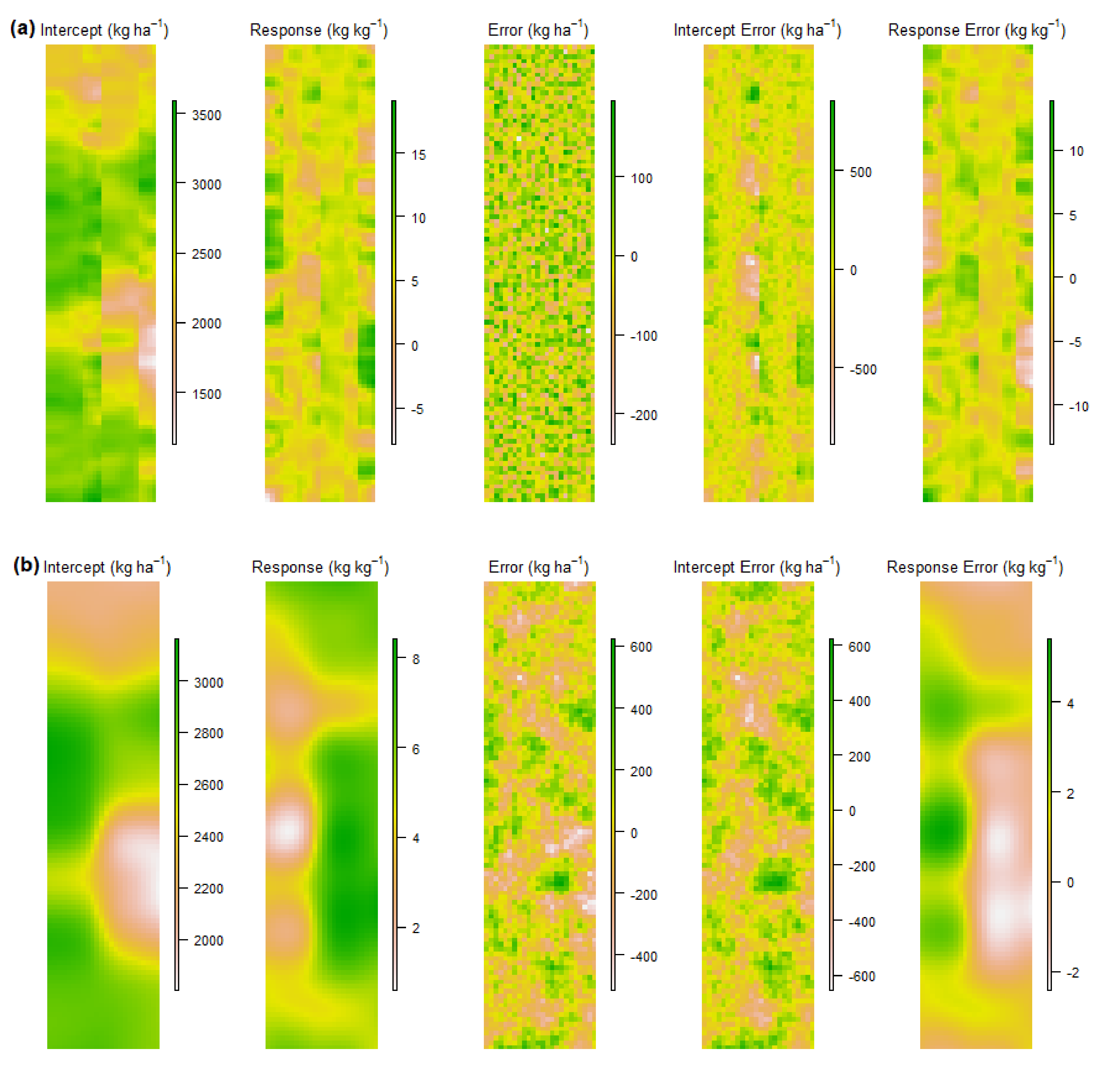
3.1. Simulated Data

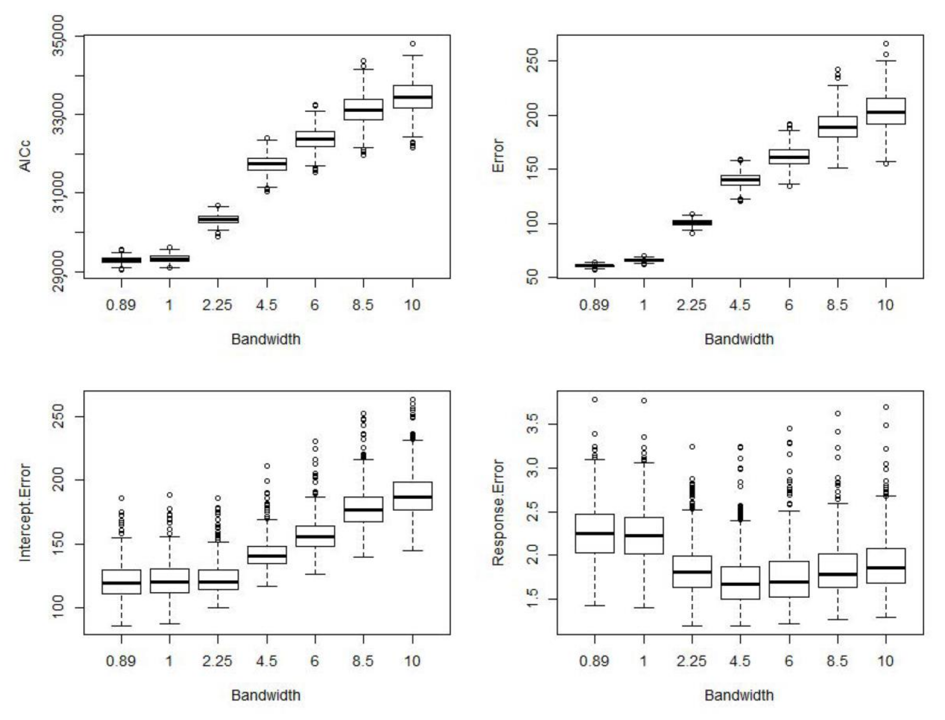
3.1.1. Bandwidth Selection

This section presents the results of applying basic GWR to three types of simulated data: global linear response, local linear response that varies across three zones, and locally varying linear response. For each simulation, the yield is modelled using a basic GWR model with a spatially varying intercept and slope (response) with a Gaussian kernel:

$$\mathrm{gwr}.\mathrm{basic}\left(\mathrm{yield}~\mathrm{rate} , \mathrm{kernel} = “\mathrm{gaussian}”, \mathrm{adaptive} = \mathrm{FALSE}\right).$$

(9)

We show maps of locally estimated intercept and slope, which we refer to as the “response” to treatment. We map the error components: overall model error and error in estimating the intercept and response. We compare the results of using two bandwidths: the bandwidth that minimises AICc (identified using GWmodel function ‘bw.gwr’) and that based on the strip width. For the simulated data, the strips are 3 pixels (30 m) wide, and using the formula in Section 2.3.2, the optimal bandwidth is given by $\left(\tau -1\right)d/2 =$4.5 pixels (45 m).

For the simulated data with global linear response to fertiliser, AICc is minimised using bandwidth = 0.87 pixels. The estimated intercepts and responses are mapped in Figure 6a with the error components. The intercept map looks like a slightly smoothed version of the minimum yield ($yield.min$). The mean of the response (estimated slope coefficient) is 5.7, which is near the constant value of 6 used to create the simulation. Estimated response ranges from −7.6 to 19.1. However, both the intercept and response maps show effects corresponding to the simulated trial strips, and there is clearly confounding between the intercept and response. The overall model error has no visible spatial autocorrelation; however, there is autocorrelation evident in the errors in the estimated intercept and response. The results using a larger bandwidth of 4.5 are shown in Figure 6b. Use of the larger bandwidth results in smoother estimates of both the intercept and response. The mean response is 5.2, but the response has a reduced range of 0.6 to 8.4. The errors in the overall model and intercept are larger and more spatially autocorrelated than when using the AICc-minimising bandwidth; however, the error in estimation of the response is smaller.

For the simulated data where the linear response is constant for three fixed zones, a bandwidth of 0.87 pixels minimised AICc. The intercept, response, and errors are shown in Figure 7a. The response map shows some error along the zone and strip boundaries. Variation within the zones is visible in the response map, but the mean response across each of the three zones is −0.6, 6.1, and 11.5, which are near the values of 0, 6, and 12 used to simulate the data. The overall error is small and has no visible spatial autocorrelation; however, spatial autocorrelation is evident in the intercept and response error. The results using the larger bandwidth are shown in Figure 7b. Use of the larger bandwidth results in smoother estimates of the intercept and response without affecting the ability of GWR to identify the mean response for each zone. While the overall error is higher than that achieved using the AICc-minimising bandwidth, the error in the intercept and response is lower.

For the simulation of locally varying linear response, AICc was minimised using a bandwidth of 0.88 pixels. The results are shown in Figure 8a. They show confounding between the estimated intercept and response, with considerable error in estimation of the response. In contrast, when the larger bandwidth is used, as shown in Figure 8b, there is no confounding between the estimated intercept and response, and although there is more spatial autocorrelation in the overall and intercept errors, the response error is lower.

Summary of Bandwidth Selection Results and Recommended Approach to Bandwidth Selection for OFE

For simulations of global linear response, linear response that varies across zones, and locally varying linear response, AICc-minimising bandwidths ranged from 0.87 to 0.88 pixels. Using AICc-minimising bandwidth, GWR on local linear response by zones showed an error in the part of the trial where the highest rate of fertiliser was applied, and GWR applied to locally varying linear response showed confounding between the estimated intercept and response. In contrast, the use of a larger bandwidth based on the width of strips in the trial resulted in smoother estimates of the intercept and response as well as more accurate estimates of response, with less confounding, despite a larger and more autocorrelated overall error. To test whether a more accurate estimation of response is an artefact of this particular simulation, we performed 500 simulations of minimum yield with locally varying linear response for bandwidths of 0.89, 1, 2.25, 4.5, 6, 8.5, and 10 pixels. The results show that AICc, overall error, and intercept error all increase with increasing bandwidth, but the response error decreases as the bandwidth increases to a minimum value achieved using bandwidth 4.5 before increasing again (Figure 9). This supports the theory presented in Section 2.3.2 with respect to determining the optimal bandwidth based on the experimental design for estimating yield response to treatment. There are also implications for the interpretation of results of GWR analyses: reduced variation in the estimated intercept and response maps when using larger bandwidths should enable easier interpretation, and end users can have greater confidence in the ability of the GWR approach to separate treatment effects from other non-treatment influences on yield.

3.1.2. Model Selection

This section tests whether model selection correctly identifies the optimal model for global and locally varying response to fertiliser. We use a Gaussian kernel with both the AICc-minimising bandwidth and bandwidth of 4.5 pixels based on the width of experimental strips.

Table 3. AICc for models of increasing order of complexity fitted to data with simulated global and locally varying linear response (minimum values of AICc identify optimal models; these are marked with asterisks, *).

Model	Global Linear (gwr.mixed)	Local Linear (gwr.basic)	Global Linear (gwr.mixed)	Local Linear (gwr.basic)
Simulated data with global linear response
Bandwidth (pixels)	0.87	0.87	4.5	4.5
AICc	28,468 *	28,795	31,397	31,227 *
Simulated data with local linear response
Bandwidth (pixels)	0.88	0.88	4.5	4.5
AICc	30,032	29,303 *	33,184	31,973 *

shows the results.

Model selection performed on the global linear simulation correctly identified the optimal model as global linear when using the optimal bandwidth identified by minimising AICc; however, when a larger bandwidth based on strip width was used, model selection failed to identify the correct model (Table 3). Model selection performed on the simulation of locally varying linear response correctly identified the optimal model as local linear using both the optimal bandwidth identified by minimising AICc and when using a larger bandwidth based on strip width.

Summary of Model Selection Results and Recommended Approach to Model Selection for OFE

Stepwise model selection identified the correct model for global response only when using the optimal bandwidth identified by minimising AICc. For locally varying response, the correct model was identified using optimal and larger bandwidths. This suggests that to determine whether the assumption of locally varying response is valid, model selection should be performed using the AICc-minimising bandwidth; then, the selected model should be estimated using a larger bandwidth. To test whether this conclusion holds, we performed 500 simulations of minimum yield with both global and local response and calculated the percentage of times model selection identified the correct model (

Table 4. Percentage of 500 simulations in which the correct model was identified by model selection.

Bandwidth	Global Response	Local Response
AICc-minimising	100	78
45 m	<1	100

). The results showed that use of the smaller AICc-minimising bandwidth correctly identified the global model 100% of the time and the local model 78% of the time. Use of the larger bandwidth led to local models being selected all of the time. Therefore, we recommend that model selection for OFE be performed as follows:

• Calculate the bandwidth that minimises AICc.
• Fit a mixed GWR that allows only the intercept to vary spatially.
• Fit a basic GWR that allows both the intercept and yield response to treatment to vary spatially.
• Select the model from 2 and 3 that has the lowest AICc.

We applied the Monte Carlo technique described in [52] to the same 500 simulations, but that method performed more poorly (

Table 5. Percentage of 500 simulations in which the correct model was identified by a Monte Carlo test for spatial variability.

Bandwidth	Global Response	Local Response
AICc-minimising	70	69
45 m	18	99

).

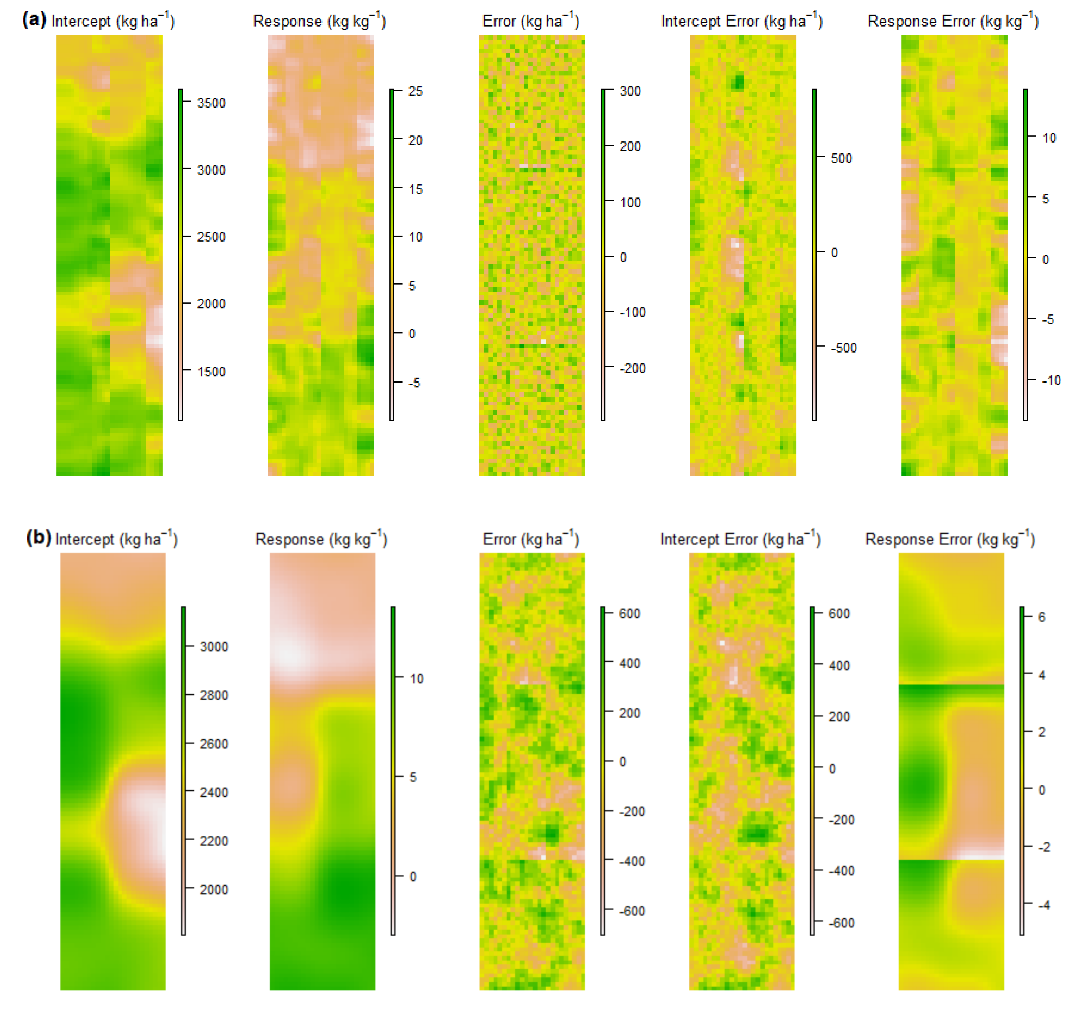
3.2. Potassium Trials

Model selection for each of the potassium trials was performed using the recommended approach developed using the simulated data in Section 3.1.2. After identifying the optimal model, GWR bandwidths were determined using the optimal approach identified using simulated data in Section 3.1.1, such that the optimal bandwidth is given by $\left(\tau -1\right)d/2$ where $\tau$ is the number of fertiliser rates being trialed and d is the width of the plot trials.

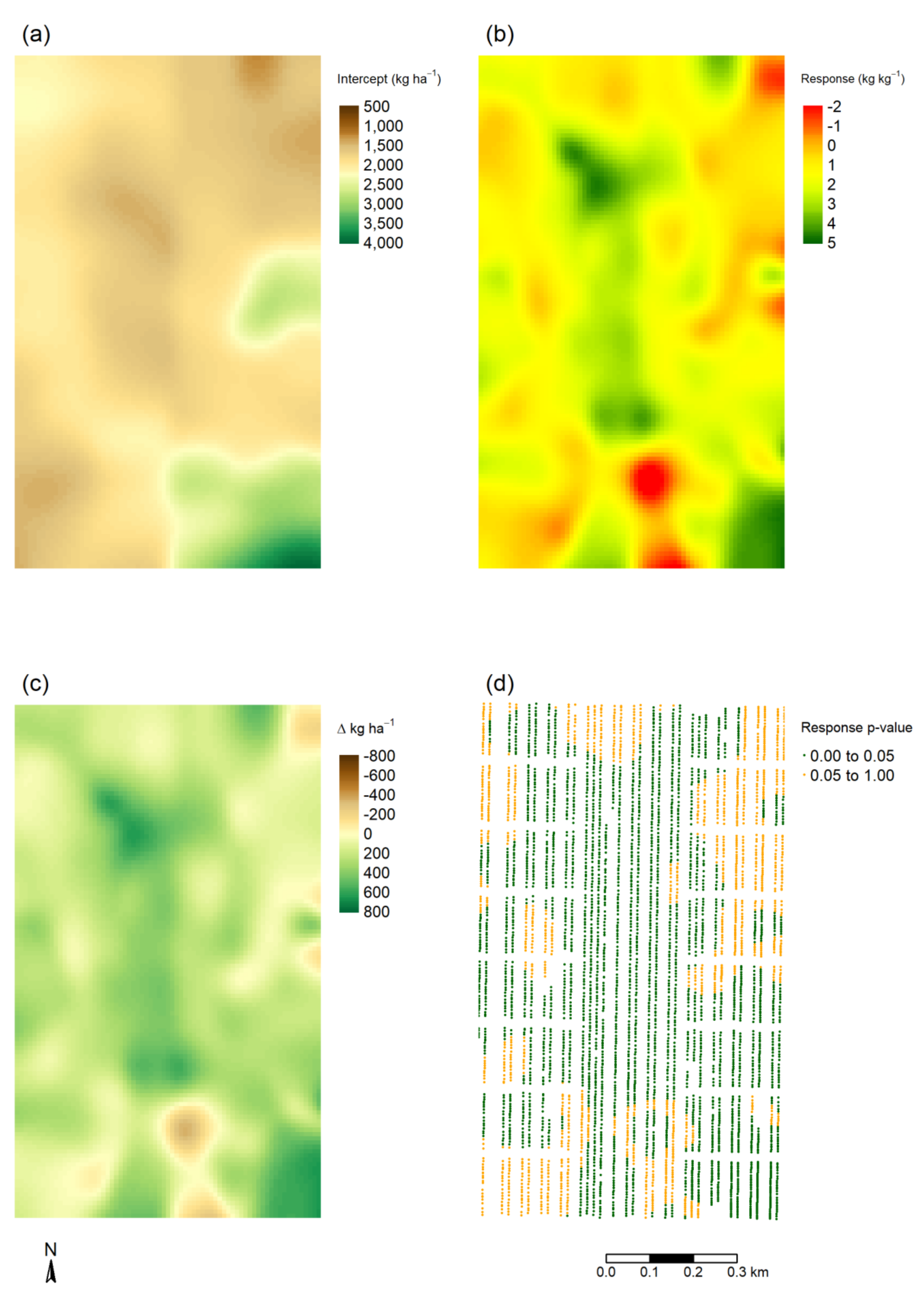
3.2.1. Cunderdin Trial

Model selection for the Cunderdin trial identified the mixed GWR model as optimal, meaning that while there was a variation in yield that was not due to fertiliser, the barley yield response to potassium was homogenous across the trial. The optimal bandwidth was 12 m. Mixed GWR was applied using this bandwidth with a non-adaptive Gaussian kernel to predict the intercept (expected yield with no fertiliser applied) over a grid of 10 m by 10 m cells across the trial area. The intercept map, shown in Figure 10a, looks like a smoothed version of the cleaned yield data. This map is the yield expected if no MOP fertiliser treatment was applied. Therefore, the spatial variation visible in the intercept map is attributed to all non-treatment effects on yield, such as the amount of stored potassium and other nutrients in the soil, soil type, and constraints. Values range from 4000 to 6000 kg ha⁻¹. The global response (rate of change in yield due to applied MOP) was 1.7 kg ha⁻¹ of barley yield per kg ha⁻¹ of MOP applied. This response is extremely low and would not justify the use of MOP fertilisation: the expected yield with no fertiliser applied is 4605 kg ha⁻¹ across the trial. The addition of 40 kg MOP ha⁻¹ would result in a total yield increase of only 61 kg ha⁻¹, and 80 kg MOP ha⁻¹ would result in an increase of only 121 kg ha⁻¹.

The model errors are shown in Figure 10b. Approximately 90% of the absolute errors are less than 500 kg ha⁻¹, and approximately 50% of the absolute errors are less than 250 kg ha⁻¹. The correlation between observed and predicted yields is 0.63.

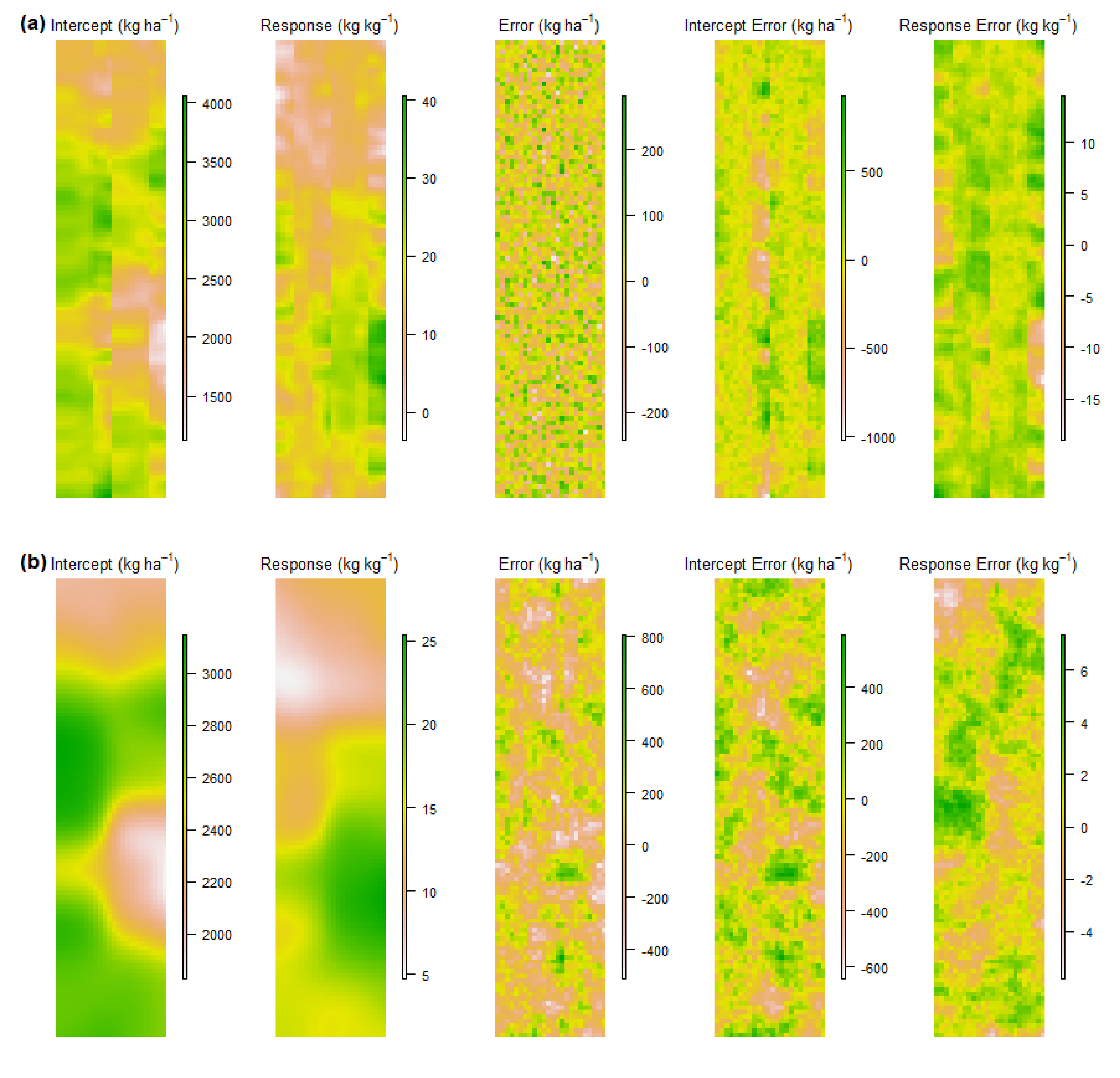
3.2.2. Narambeen Trial

Model selection for the Narambeen trial identified the basic GWR model as optimal, meaning that the yield response to treatment varies spatially across the trial. Each plot contained two swathes of yield data, so the plots are 30 m wide, and therefore, the optimal bandwidth is 45 m. Basic GWR was applied using this bandwidth with a non-adaptive Gaussian kernel to predict the intercept and response over a grid of 10 m by 10 m cells across the trial area. The intercept map shown in Figure 11a looks like a smoothed version of the cleaned yield data. This map is the yield expected if no MOP fertiliser treatment was applied. Therefore, the spatial variation visible in the intercept map is attributed to all non-treatment effects on wheat yield, such as soil nutrition, soil type, and management constraints. Values range from 500 to 4000 kg ha⁻¹, with three quarters of the paddock yielding less than 2000 kg ha⁻¹.

The response map, shown in Figure 11b, shows the rate at which applied MOP will affect yield (the slope of the local regressions). Across 95% of the trial area, MOP had a positive yield response. Local t-tests, shown in Figure 11d, showed that the effect of fertiliser on yield was significant (p < 0.05) over 75% of the trial area. However, the mean response was only 1.6 kg yield ha⁻¹ per kg of MOP applied, and the maximum response is 5 kg ha⁻¹ yield per kg of MOP applied. A recent analysis of potassium cost to wheat grain prices [69] showed that the that the break-even ratio for the fertilisation of barley with MOP was 7.4; thus, this analysis shows that MOP fertilisation is not profitable for this paddock. This begs the question: Is statistical significance as important as practical or economic significance? Since farmers are ultimately interested in profit, statistical significance is not necessarily a useful piece of information for OFE.

GWR can be used to predict yield using different amounts of fertiliser by application of the regression equation; for example, Figure 11c shows the predicted change in yield if 134 kg ha⁻¹ of MOP had been applied. The predicted average improvement in yield achieved across the trial by MOP fertiliser application was 106 kg ha⁻¹ at a rate of 66 kg MOP ha⁻¹, 215 kg ha⁻¹ at a rate of 134 kg MOP ha⁻¹, and 321 kg ha⁻¹ at 200 kg MOP ha⁻¹.

Model errors ranged from -1519 to 1709 kg ha⁻¹ with 90% of absolute errors less than 275 ha⁻¹. The correlation between observed and predicted yields is 0.90.

4. Discussion

A major benefit of OFE is that it provides substantially more information about performance at the field scale than conventional plot trials and thereby supports a direct interpretation of manageable effects. However, the additional complexity this information provides can make analysis challenging. Using simulation, this work has shown that GWR is a simple method for the analysis of OFE data that can accurately separate yield variation that is not due to the applied treatment from yield response due to treatment. A process of model selection can be used to determine whether yield response to treatment is constant across the trial or spatially varying. The GWR method is relatively easy to apply to large-scale on-farm experiments. It accepts a range of experimental designs that can be easily installed in commercial operations.

The method requires some care in application, particularly in bandwidth and model selection. In Section 3.1.1, we considered bandwidth selection for OFE and showed that the standard method that selects bandwidth by minimising AICc is sub-optimal for an analysis of OFE data, which are densely and regularly distributed in space. We tested a simple method for bandwidth selection based on trial design [48] and found that the larger bandwidths it prescribes are better able to separate treatment and non-treatment effects and provide more accurate estimates of yield response to treatment. The results presented here are similar to those obtained by Guo et al. [70], who concluded that AIC minimisation may not be optimal for bandwidth selection, and smaller bandwidths can overfit local models.

While conventional agronomic research seeks to represent underlying global truths about relationships between treatments and crop growth, we hypothesise that a spatially variable treatment–yield relationship will be appropriate in most cases, because factors controlling crop yield vary continuously in space and results obtained from any one location may not apply to new locations. Furthermore, decades of observation of crop yield variation from precision agriculture indicate a large spatial variation within and between management units. We test this hypothesis using model selection to compare basic GWR models that assume that yield response varies locally with mixed GWR models where response is assumed to be global across the trial. Our recommended approach for model selection did not give perfect results on simulated data: while it correctly identified simulations of global response with 100% accuracy, it only identified simulations of local response 78% of the time. We also tried a commonly used Monte Carlo technique [52], but that method performed more poorly.

When applied to two on-farm experiments that aimed to investigate yield response to MOP fertiliser, our recommended bandwidth and model selection approaches identified one trial as having global response and one as having local response. For each, the GWR intercept map estimated a variation in yield that was not due to treatment. The overall error for modelling each trial was low, and the R² was 0.63 for the Cunderdin trial and 0.9 for the Narambeen trial, which compares favourably with another published potassium-yield model derived from on-farm experiments, which had an R² of 0.48 [71]. Unfortunately, both of our potassium trials showed small yield responses to MOP fertiliser; and moreover, a response that was below the break-even ratio, indicating that fertilisation with MOP was not profitable at either location. This may because there was sufficient plant-available potassium in the soil, and it would be useful to compare the results of soil tests taken prior to experimentation with locally varying response in future trials. We intend to follow up this study by applying our recommended approach in situations where larger yield responses might be expected—for example, nitrogen trials in known deficient conditions. We note that while our applications are in broadacre cereal cropping, OFE can also be used for any horticultural or viticultural cropping system.

One concern is that while the estimation of basic GWR models is fast, the estimation of mixed GWR models and their AICc values can be slow for the large datasets acquired from OFE (approximately 40 min for our simulated data compared to less than one minute using basic GWR on a Dell Latitude laptop with 2.8 GHz CPU and 32 GB RAM). This has implications for the widespread practical application of GWR and its implementation in computer software. The importance of model selection is demonstrated in Section 3.1.2, and the use of an incorrect model could lead to spurious management decisions by the farmer. However, while the use of a mixed GWR model applied to simulated data with locally varying response gave poor results, basic GWR applied to simulated data with a global response gave realistic results that estimated the mean response equal to the global response used to simulate the data. This means that incorrectly applying a basic GWR model results in a smaller error than incorrectly applying a mixed GWR model. In practice, the likelihood of misinterpreting the results of simply applying basic GWR to OFE will be further reduced by several factors.

First, because on-farm experiments are conducted at the same scale as conventional management, the framework for evaluating results parallels the knowledge farmers use to make sense of complex information about the landscape they manage. Farmers and consultants draw information from a wide range of sources to reduce uncertainty [14]. While formal models can contribute much to support this decision-making under uncertainty, the end result will rely strongly on intuition that can be assisted by large-scale visualisations [72].

Second, the information that is extracted from OFE will vary depending on its purpose and context. While OFE may be used to support PA zoning, there are many other potential benefits from the learning around them, including the confirmation of suspected performance trends; the identification of specific treatment by soil interactions; or the use of results as performance indicators.

Thirdly is the question of practical significance of measured variation. A farmer, aided by an agronomic consultant [73], might conclude that the range of statistically significant response revealed by basic GWR was of interest but not large enough to require localised (PA) fertiliser management. That conclusion could be driven by practicality or economic considerations (as for the potassium trials we report) rather than statistical confidence, meaning that model selection for OFE could become part of the interpretation of results as well as part of the analysis. In that case, basic GWR could be quickly and easily applied to OFE in a semi-automated way to support decision-making. We use the term “semi-automated” because data analysis using GWR can be automated within a software platform, but interpretation of the results, assessment of the practical significance of results, and implications of the results for decision-making are all critical parts of the co-learning OFE process that cannot be automated. While the development of computer software for data analysis is possible and desirable, OFE is a larger process that requires systems for ongoing engagement, communication, and agronomic assistance in interpreting the results of analysis.

OFE is part of a learning process that is incremental in nature. Each experiment and analysis provides information about part of a complex managed system. Within this continued learning process, OFE results can lead to more questions being asked about the causes of spatial variability in yield response to treatment and spatial variability in yield that is not due to treatment. This in turn leads to more experiments being designed and conducted, in an ongoing cycle of knowledge development. For this, OFE requires easy-to-implement methods that can provide value from the process, even while more sophisticated methods emerge. In the early stages of this cycle, basic GWR analyses such as those described in this paper can provide sufficient learning to support this cycle as it progresses. We anticipate that as the experimental questions diversify, more complex methods of analysis can and should be sought.

By estimating local linear response curves, GWR can be used to predict the effects of different rates of fertiliser application. In this, it differs from geostatistical applications that interpolate yields from different treatments onto a common grid and then perform point-wise hypothesis testing [46,74]. However, fertiliser response is typically only linear in the part of the response curve before the rate of the response diminishes and a maximum yield is attained. The rate of fertiliser that maximises profits is lower that the yield-maximising rate, and it usually lies in the non-linear part of the response curve [75]. Thus, targeting just the linear part of the response curve omits consideration of the section of response that determines optimal management: that is, identification of the economic break-even ratio and profit-maximising rate. Local non-linear response curves can potentially be fitted to co-kriged yield maps from different treatments [44]. Based on the results of this study, we surmise that non-linearity can also be supported within a GWR framework by incorporating distance-based spatial weights in non-linear rather than linear regression. We are extending the GWR framework to this end and comparing GWR with other methods for analysis (linear, non-linear, and geostatistical) of data from large on-farm experiments in future work.

The use of additional data sources to attribute causes of variation is also required. These may include information about soil nutrition from soil samples taken prior to experimentation that can be used to tailor local response curves or other spatial data that can be used to explain non-fertiliser causes of spatial variability in yield. Ideally, the identification of suitable data sources for testing would become a part of the OFE co-learning framework.

5. Conclusions

OFE is an inexpensive means of acquiring knowledge to support on-farm decision-making and improve the uptake of digital agriculture. The process appeals to farmers, but an analysis of data from OFE can be challenging. GWR is a relatively simple method for testing for and modelling spatial variability in yield response that provides a pragmatic solution to this challenge. It has the advantage that it can be easily explained to farmers and their advisors.

Similar to all pragmatic solutions, the use of GWR requires judgment in the selection of appropriate approaches to application. This article used simulated data to show that GWR can accurately separate non-treatment and treatment effects and test approaches for bandwidth and model selection for GWR applied to OFE data, thereby developing more consistent methodologies for analysis that facilitate interpretation and subsequent farmer decision-making. It demonstrated the application of these methodologies on data from two potassium trials in Western Australia. Based on these results, we assert that GWR has the potential to be widely applied in a semi-automated manner to analyse OFE data, enhance adoption of digital technologies, and improve farm productivity and profitability.

Furthermore, rigorous statistical analysis of on-farm experiments using GWR as a base will enable agricultural researchers to use large on-farm trials to support the generation of agricultural knowledge and hypothesis testing at scale.

References

- Robert, P.C. Precision agriculture: A challenge for crop nutrition management. Plant Soil 2002, 247, 143–149. [Google Scholar] [CrossRef]
- International Society of Precision Agriculture. Available online: https://www.ispag.org/ (accessed on 1 June 2019).
- Cook, S.E.; Bramley, R.G.V. Precision agriculture-opportunities, benefits and pitfalls of site-specific crop management in Australia. Aust. J. Exp. Agric. 1998, 38, 753–763. [Google Scholar] [CrossRef]
- Robertson, M.J.; Llewellyn, R.S.; Mandel, R.; Lawes, R.; Bramley, R.G.V.; Swift, L.; Metz, N.; O’Callaghan, C. Adoption of variable rate fertiliser application in the Australian grains industry: Status, issues and prospects. Precis. Agric. 2011, 13, 181–199. [Google Scholar] [CrossRef]
- McBratney, A.B.; Whelan, B.; Ancev, T.; Bouma, J. Future directions of precision agriculture. Precis. Agric. 2005, 6, 7–23. [Google Scholar] [CrossRef]
- Bramley, R.G.V.; Ouzman, J. Farmer attitudes to the use of sensors and automation in fertilizer decision-making: Nitrogen fertilization in the Australian grains sector. Precis. Agric. 2019, 20, 157–175. [Google Scholar] [CrossRef]
- Cock, J.; Oberthür, T.; Isaacs, C.; Läderach, P.R.; Palma, A.; Carbonell, J.; Victoria, J.; Watts, G.; Amaya, A.; Collet, L.; et al. Crop management based on field observations: Case studies in sugarcane and coffee. Agric. Syst. 2011, 104, 755–769. [Google Scholar] [CrossRef]
- Jimenez, D.; Dorado, H.; Cock, J.; Prager, S.D.; Delerce, S.; Grillon, A.; Andrade Bejarano, M.; Benavides, H.; Jarvis, A. From observation to information: Data-driven understanding of on farm yield variation. PLoS ONE 2016, 11, e0150015. [Google Scholar] [CrossRef]
- Lamb, D.W.; Frazier, P.; Adams, P. Improving pathways to adoption: Putting the right P’s in precision agriculture. Comput. Electron. Agric. 2008, 61, 4–9. [Google Scholar] [CrossRef]
- Pannell, D.J.; Marshall, G.R.; Barr, N.; Curtin, A.; Vanclay, F.; Wilkinson, R. Understanding and promoting adoption of conservation practices by rural landholders. Aust. J. Exp. Agric. 2006, 46, 1407–1424. [Google Scholar] [CrossRef]
- Kutter, T.; Tiemann, S.; Siebert, R.; Fountas, S. The role of communication and co-operation in the adoption of precision farming. Precis. Agric. 2009, 12, 2–17. [Google Scholar] [CrossRef]
- Paustian, M.; Theuvsen, L. Adoption of precision agriculture technologies by German crop farmers. Precis. Agric. 2016, 18, 701–716. [Google Scholar] [CrossRef]
- Pierpaoli, E.; Carli, G.; Pignatti, E.; Canavari, M. Drivers of precision agriculture technologies adoption: A literature review. Procedia Technol. 2013, 8, 61–69. [Google Scholar] [CrossRef]
- Cook, S.; Cock, J.; Oberthür, T.; Fisher, M. On-farm experimentation. Better Crops 2013, 4, 17–20. [Google Scholar]
- Cook, S.; Lacoste, M.; Evans, F.; Ridout, M.; Gibberd, M.; Oberthür, T. An on-farm experimental philosophy for farmer-centric digital innovation. In Proceedings of the 14th International Conference on Precision Agriculture, Montreal, QC, Canada, 24–27 June 2018. [Google Scholar]
- Sylvester-Bradley, R.; Kindred, D.R.; Marchant, B.; Rudolph, S.; Roques, S.; Calatayud, A.; Clarke, S.; Gillingham, V. Agronōmics: Transforming crop science through digital technologies. Adv. Anim. Biosci. 2017, 8, 728–733. [Google Scholar] [CrossRef]
- Kyveryga, P.M. On-farm research: Experimental approaches, analytical frameworks, case studies, and impact. Agron. J. 2019, 111, 2633–2635. [Google Scholar] [CrossRef]
- Bullock, D.S.; Boerngen, M.; Tao, H.; Maxwell, B.; Luck, J.D.; Shiratsuchi, L.; Puntel, L.; Martin, N.F. The data-intensive farm management project: Changing agronomic research through on-farm precision experimentation. Agron. J. 2019, 111, 2736–2746. [Google Scholar] [CrossRef]
- Schmidt, P.; Möhring, J.; Koch, R.J.; Piepho, H.P. More, larger, simpler: How comparable are on-farm and on-station trials for cultivar evaluation? Crop Sci. 2018, 58, 1508–1518. [Google Scholar] [CrossRef]
- Marchant, B.; Rudolph, S.; Roques, S.; Kindred, D.; Gillingham, V.; Welham, S.; Coleman, C.; Sylvester-Bradley, R. Establishing the precision and robustness of farmers’ crop experiments. Field Crops Res. 2019, 230, 31–45. [Google Scholar] [CrossRef]
- Cook, S.E.; Adams, M.L.; Corner, R.J. On-farm experimentation to determine site-specific responses to variable inputs. In Proceedings of the 4th International Conference on Precision Agriculture, Minneapolis, MN, USA, 19–22 July 1998; pp. 611–621. [Google Scholar]
- Lawes, R.A.; Bramley, R.G.V. A simple method for the analysis of on-farm strip trials. Agron. J. 2012, 104, 371–377. [Google Scholar] [CrossRef]
- Hall, D.; Galloway, P.; Lemon, J.; Curtis, B.; van Burgel, A.; Kong, K. The Agronomy Jigsaw: Finding the Pieces That Maximise Water Use Efficiency; Department of Agriculture and Food, Government of Western Australia (DAFWA): Kensington, Australia, 2014. [Google Scholar]
- Sela, S.; van Es, H.M.; Moebius-Clune, B.N.; Marjerison, R.; Melkonian, J.; Moebius-Clune, D.; Schindelbeck, R.; Gomes, S. Adapt-N outperforms grower-selected nitrogen rates in northeast and midwestern United States strip trials. Agron. J. 2016, 108, 1726–1734. [Google Scholar] [CrossRef]
- Whelan, B.M.; Taylor, J.A.; McBratney, A.B. A ‘small strip’ approach to empirically determining management class yield response functions and calculating the potential financial ‘net wastage’ associated with whole-field uniform-rate fertiliser application. Field Crops Res. 2012, 139, 47–56. [Google Scholar] [CrossRef]
- Bramley, R.; Cook, S.; Adams, M.; Corner, R. Designing Your Own on-Farm Experiments; Grains Research and Development Corporation: Canberra, Australia, 1999. [Google Scholar]
- Doerge, T.A.; Gardner, D.L. On-farm testing using the adjacent strip comparison method. In Proceedings of the 4th International Conference on Precision Agriculture, Minneapolis, MN, USA, 19–22 July 1998; pp. 603–609. [Google Scholar]
- Schwenke, G.; Beange, L.; Cameron, J.; Bell, M.; Harden, S.; Aitkenhead, M. What soil information do crop advisors use to develop nitrogen fertilizer recommendations for grain growers in New South Wales, Australia? Soil Use Manag. 2019, 35, 85–93. [Google Scholar] [CrossRef]
- Adams, M.L.; Cook, S.E. Methods of on-farm experimentation. In Proceedings of the ASAE Annual International Meeting, Minneapolis, MN, USA, 10–14 August 1997. [Google Scholar]
- Kindred, D.; Sylvester-Bradley, R.; Clarke, S.; Roques, S.; Smillie, I.; Berry, P. Agronōmics—An arena for synergy between the science and practice of crop production. In Proceedings of the 12th European IFSA Symposium, Harper Adams University, New Port, UK, 12–16 July 2016. [Google Scholar]
- Fisher, R.A. The arrangement of field experiments. J. Minist. Agric. Great Br. 1926, 33, 503–513. [Google Scholar]
- Oehlert, G.W. A First Course in the Design and Analysis of Experiments; University of Minnesota Digital Conservancy: Minneapolis, MN, USA, 2010. [Google Scholar]
- Kravchenko, A.N.; Snapp, S.S.; Robertson, G.P. Field-scale experiments reveal persistent yield gaps in low-input and organic cropping systems. Proc. Natl. Acad. Sci. USA 2017, 114, 926–931. [Google Scholar] [CrossRef]
- Piepho, H.-P.; Richter, C.; Spilke, J.; Hartung, K.; Kunick, A.; Thöle, H. Statistical aspects of on-farm experimentation. Crop Pasture Sci. 2011, 62, 721–735. [Google Scholar] [CrossRef]
- Tobler, W.R. A computer movie simulating urban growth in the Detroit region. Econ. Geogr. 1970, 46, 234–240. [Google Scholar] [CrossRef]
- Gilmour, A.R.; Cullis, B.R.; Verbyla, A.P. Accounting for natural and extraneous variation in the analysis of field experiments. J. Agric. Biol. Environ. Stat. 1997, 2, 269. [Google Scholar] [CrossRef]
- Piepho, H.-P.; Williams, E.R.; Michel, V. Beyond Latin squares: A brief tour of row-column designs. Agron. J. 2015, 107, 2263–2270. [Google Scholar] [CrossRef]
- Van Frank, G.; Goldringer, I.; Rivière, P.; David, O. Influence of experimental design on decentralized, on-farm evaluation of populations: A simulation study. Euphytica 2019, 215, 126. [Google Scholar] [CrossRef]
- Anselin, L.; Bogiovanni, R.; Lowenberg-deBoer, J. A spatial econometric approach to the economics of site-specific nitrogen management in corn production. Am. J. Agric. Econ. 2004, 86, 675–687. [Google Scholar] [CrossRef]
- Lambert, D.M.; Lowenberg-Deboer, J.; Bongiovanni, R. A comparison of four spatial regression models for yield monitor data: A case study from Argentina. Precis. Agric. 2004, 5, 579–600. [Google Scholar] [CrossRef]
- Griffin, T.W.; Dobbins, C.L.; Vyn, T.J.; Florax, R.J.G.M.; Lowenberg-DeBoer, J.M. Spatial analysis of yield monitor data: Case studies of on-farm trials and farm management decision making. Precis. Agric. 2008, 9, 269–283. [Google Scholar] [CrossRef]
- Jiang, P.; He, Z.; Kitchen, N.R.; Sudduth, K.A. Bayesian analysis of within-field variability of corn yield using a spatial hierarchical model. Precis. Agric. 2008, 10, 111–127. [Google Scholar] [CrossRef]
- Lark, R.M.; Wheeler, H.C. A method to investigate within-field variation of the response of combinable crops to an input. Agron. J. 2003, 95, 1093–1104. [Google Scholar] [CrossRef]
- Pringle, M.J.; McBratney, A.B.; Cook, S.E. Field-scale experiments for site-specific crop management. Part II: A geostatistical analysis. Precis. Agric. 2004, 5, 625–645. [Google Scholar] [CrossRef]
- Panten, K.; Bramley, R.G.V.; Lark, R.M.; Bishop, T.F.A. Enhancing the value of field experimentation through whole-of-block designs. Precis. Agric. 2010, 11, 198–213. [Google Scholar] [CrossRef]
- Bishop, T.F.A.; Lark, R.M. The geostatistical analysis of experiments at the landscape-scale. Geoderma 2006, 133, 87–106. [Google Scholar] [CrossRef]
- Rudolph, S.; Marchant, P.B.; Gillingham, V.; Kindred, D.; Sylvester-Bradley, R. Spatial discontinuity analysis, a novel geostatistical algorithm for on-farm experimentation. In Proceedings of the 13th International Conference on Precision Agriculture, Monticello, IL, USA, 31 July–3 August 2016. [Google Scholar]
- Rakshit, S.; Baddeley, A.; Stefanova, K.; Reeves, K.; Chen, K.; Cao, Z.; Evans, F.; Gibberd, M. Novel approach to the analysis of spatially-varying treatment effects in on-farm experiments. Field Crops Res. 2020, 255, 107783. [Google Scholar] [CrossRef]
- Trevisan, R.G.; Bullock, D.S.; Martin, N.F. Spatial variability of crop responses to agronomic inputs in on-farm precision experimentation. Precis. Agric. 2020, 1–22. [Google Scholar] [CrossRef]
- Brunsdon, C.; Fotheringham, S.; Charlton, M. Geographically weighted regression: A method for exploring spatial nonstationarity. Geogr. Anal. 1996, 28, 281–298. [Google Scholar] [CrossRef]
- Brunsdon, C.; Fotheringham, S.; Charlton, M. Geographically weighted regression—Modelling spatial non-stationarity. J. R. Stat. Soc. Ser. D (Stat.) 1998, 47, 431–443. [Google Scholar] [CrossRef]
- Fotheringham, S.; Brunsdon, C.; Charlton, M. Geographically Weighted Regression: The Analysis of Spatially Varying Relationships; Wiley: Hoboken, NJ, USA, 2002. [Google Scholar]
- Mitscherlich, E.A. Das gesetz des minimums und das Gesetz des abnehmenden Bodenertrages (Eng: The law of the minimum and the law of diminishing soil productivity). Landwirtsch. Jahrbücher 1909, 38, 537–552. [Google Scholar]
- Tembo, G.; Brorsen, B.W.; Epplin, F.M.; Tostão, E. Crop input response functions with stochastic plateaus. Am. J. Agric. Econ. 2008, 90, 424–434. [Google Scholar] [CrossRef]
- Bullock, D.G.; Bullock, D.S. Quadratic and quadratic-plus-plateau models for predicting optimal nitrogen rate of corn: A comparison. Agron. J. 1994, 86, 191–195. [Google Scholar] [CrossRef]
- Sylvester-Bradley, R.; Kindred, D.R.; Wynn, S.C.; Thorman, R.E.; Smith, K.E. Efficiencies of nitrogen fertilizers for winter cereal production, with implications for greenhouse gas intensities of grain. J. Agric. Sci. 2012, 152, 3–22. [Google Scholar] [CrossRef]
- Robertson, M.J.; Lyle, G.; Bowden, J.W. Within-field variability of wheat yield and economic implications for spatially variable nutrient management. Field Crop. Res. 2008, 105, 211–220. [Google Scholar] [CrossRef]
- Akaike, H. Information theory and an extension of the maximum likelihood principle. In Proceedings of the Second International Symposium on Information Theory, Tsahkadsor, Armenia, 2–8 September 1971; pp. 267–281. [Google Scholar]
- Brunsdon, C.; Fotheringham, S.; Charlton, M. Geographically Weighted Regression as a Statistical Model; Newcastle University: Newcastle, UK, 2000. [Google Scholar]
- Valavi, R.; Elith, J.; Lahoz-Monfort, J.J.; Guillera-Arroita, G.; Warton, D. blockCV: An R package for generating spatially or environmentally separated folds for k-fold cross-validation of species distribution models. Methods Ecol. Evol. 2018, 10, 225–232. [Google Scholar] [CrossRef]
- Brunsdon, C.; Fotheringham, A.S.; Charlton, M. Some notes on parametric significance tests for geographically weighted regression. J. Reg. Sci. 1999, 39, 497–524. [Google Scholar] [CrossRef]
- Mei, C.-L.; He, S.-Y.; Fang, K.-T. A note on the mixed geographically weighted regression model. J. Reg. Sci. 2004, 44, 143–157. [Google Scholar] [CrossRef]
- Gollini, I.; Lu, B.; Charlton, M.; Brunsdon, C.; Harris, P. GWmodel: An R package for exploring spatial heterogeneity using geographically weighted models. J. Stat. Softw. 2015, 63, 1–50. [Google Scholar] [CrossRef]
- Lu, B.; Harris, P.; Charlton, M.; Brunsdon, C. The GWmodel R package: Further topics for exploring spatial heterogeneity using geographically weighted models. Geo Spat. Inf. Sci. 2014, 17, 85–101. [Google Scholar] [CrossRef]
- Páez, A.; Uchida, T.; Miyamoto, K. A general framework for estimation and inference of geographically weighted regression models: 1. Location-specific kernel bandwidths and a test for locational heterogeneity. Environ. Plan. A 2002, 34, 733–754. [Google Scholar] [CrossRef]
- Da Silva, A.R.; Fotheringham, A.S. The multiple testing issue in geographically weighted regression. Geogr. Anal. 2016, 48, 233–247. [Google Scholar] [CrossRef]
- Stone, M. An asymptotic equivalence of choice of model by cross-validation and Akaike’s criterion. J. R. Stat. Soc. Ser. B 1977, 39, 44–47. [Google Scholar] [CrossRef]
- Leung, Y.; Mei, C.-L.; Zhang, W.-X. Statistical tests for spatial nonstationarity based on the geographically weighted regression model. Environ. Plan. A Econ. Space 2000, 32, 9–32. [Google Scholar] [CrossRef]
- Scanlan, C.A.; Bell, R.W.; Brennan, R.F. Simulating wheat growth response to potassium availability under field conditions in sandy soils. II. Effect of subsurface potassium on grain yield response to potassium fertiliser. Field Crops Res. 2015, 178, 125–134. [Google Scholar] [CrossRef]
- Guo, L.; Ma, Z.; Zhang, L. Comparison of bandwidth selection in application of geographically weighted regression: A case study. Can. J. For. Res. 2008, 38, 2526–2534. [Google Scholar] [CrossRef]
- Wong, M.T.F.; Corner, R.J.; Cook, S.E. A decision support system for mapping the site-specific potassium requirement of wheat in the field. Aust. J. Exp. Agric. 2001, 41, 655–661. [Google Scholar] [CrossRef]
- McCown, R.L.; Carberry, P.S.; Dalgliesh, N.P.; Foale, M.A.; Hochman, Z. Farmers use intuition to reinvent analytic decision support for managing seasonal climatic variability. Agric. Syst. 2012, 106, 33–45. [Google Scholar] [CrossRef]
- Llewellyn, R.S.; Ouzman, J. Adoption of Precision Agriculture-Related Practices: Status, Opportunities and the Role of Farm Advisers; CSIRO: Canberra, Australia, 2014. [Google Scholar]
- Bishop, T.F.A.; Lark, R.M. A landscape-scale experiment on the changes in available potassium over a winter wheat cropping season. Geoderma 2007, 141, 384–396. [Google Scholar] [CrossRef]
- Pannell, D.J. Economic perspectives on nitrogen in farming systems: Managing trade-offs between production, risk and the environment. Soil Res. 2017, 55, 473. [Google Scholar] [CrossRef]