Article

Predicting Streamflow and Nutrient Loadings in a Semi-Arid Mediterranean Watershed with Ephemeral Streams Using the SWAT Model

1
CREA Research Centre for Agricultural Policies and Bioeconomy, Via Po 14, 00198 Rome, Italy
2
FAO Food and Agriculture Organization of the United Nations, Viale delle Terme di Caracalla, 00153 Rome, Italy
3
DAGRI Department of Agriculture, Food, Environment and Forestry, University of Florence, 50144 Florence, Italy
*
Author to whom correspondence should be addressed.
Agronomy 2020, 10(1), 2; https://doi.org/10.3390/agronomy10010002
Submission received: 30 November 2019 / Revised: 13 December 2019 / Accepted: 16 December 2019 / Published: 18 December 2019

Abstract

:
Predicting the availability and quality of freshwater resources is a pressing concern in the Mediterranean area, where a number of agricultural systems depend solely on precipitation. This study aims at predicting streamflow and nonpoint pollutant loads in a temporary river system in the Mediterranean basin (Sulcis area, Sardinia, Italy). Monthly discharge, suspended sediment, nitrate nitrogen, total nitrogen, mineral phosphorus, and dissolved oxygen in-stream monitoring data from gauge stations were used to calibrate and validate the Soil and Water Assessment Tool model for the period 1979–2009. A Sequential Uncertainty Fitting procedure was used to auto-calibrate parameter uncertainties and model evaluation. Monthly simulation during the validation period showed a positive model performance for streamflow with Nash–Sutcliffe efficiency and percent bias values of 0.7% and 18.7%, respectively. The simulation results at a watershed level indicate that the sediment load was 1.13 t ha−1 year−1, while for total nitrogen and total phosphorus, the simulated values were 4.8 and 1.18 kg ha−1 year−1, respectively. These results were consistent with the values of soil and nutrient losses observed in the Mediterranean area, although hot-spot areas with high nutrient loadings were identified. The calibrated model could be used to assess long-term impacts on water quality associated with the simulated land use scenarios.

Graphical Abstract

1. Introduction

Freshwater availability and water quality play a critical role in ecosystem processes and related services worldwide. In the Mediterranean area and south-western Europe, the increasing frequency of drought events and related hazards and risks could affect the water supply (i.e., precipitation) and atmospheric water vapor demand (i.e., evapotranspiration) and, in turn, river flow and soil moisture dynamics [1]. Of particular concern are the direct effects on temporary water resources, characterized by the recurrent onset and cessation of flow [2]. Apart from the effects on biotic communities, there is a growing interest in long-term hydrological dynamics in intensive-agriculture watersheds. Extensive research has shown that environmental processes governed by water flow, such as sediment loads and nitrogen and phosphorus discharges in these environments, could seriously exacerbate freshwater and groundwater pollution, salinity, and soil erosion [3,4,5,6]. The indirect effects of the modified freshwater flux and water supply associated with the local climates’ uncertainties will induce changes in plant growth and the productivity of crops due to drought and heat stress [7]. Again, contrasting climate-driven land use changes and human pressure might increase the magnitude of land degradation and associated ecosystem functions and services in the Mediterranean drylands [8,9]. This issue is particularly pressing for Mediterranean farmers and their ‘adaptive capacity’ to deal with water scarcity [10], considering that the expected effects of climate change at a regional level could result in lower farm incomes compared to northern regions [11], in turn resulting in regional imbalances and economic winners and losers [12]. One of the greatest challenges in these areas is the development of pragmatic mitigation strategies and sustainable management options for resolving the competing claims on bioresource availability and water demands [13].
In this sense, some adaptation strategies promote land use scenarios and sustainable landscape designs integrating biomass and bioenergy production on marginal and underutilized lands into semi-arid environments [14,15]. These scenarios allocate both bioenergy and food crops across the landscape with the aim of maximizing ecosystem services and yields, and in the meantime, resolve land and water use competition. Land suitability evaluation for spatial configuration helps the shift from “land-sharing” to “land-sparing” strategies [16]. Notwithstanding the importance of a holistic evaluation of the environmental sustainability with key indicators [17], bioenergy value chain studies in European countries have tended to focus on economic analyses, the potential biomass yield and quality, the energy balance, greenhouse gas emissions, and logistics management [15,18,19]. Less attention has been paid to addressing sustainability aspects linked to the water–Energy nexus with spatially explicit land use management analyses. However, despite the growing interest in supporting bioenergy crops promoted by governmental mandates and European policies [20], ongoing and emerging issues concerning agricultural nonpoint source pollution, water resources and related use efficiency, and water quality and its sustainable use in a scenario of large-scale bioenergy crop expansion have been highlighted [21].
Against this background, the use of modeling approaches at the watershed scale is fundamental for enabling decision-makers to address environmental issues related to actual land management practices or for testing the future implementation of best management practices and alternative scenarios. Several water quality models have been used worldwide by researchers and government agencies to investigate a range of ecosystems (e.g., ponds, wetlands, and reservoirs), model processes (e.g., erosion, evapotranspiration, and nutrient modeling), and scenario analyses (e.g., crop rotation and fertilizer application) at different geographical scales. Process-based catchment models can simulate water fluxes and water-quality variables like sediments, nitrogen, phosphorus, pesticide balances, metals, pH, salts, pathogens, algal biomass, and the dissolved oxygen concentration for rivers and receiving waterbodies. A recent literature review on water quality and erosion models [22] confirms that the Soil and Water Assessment Tool (SWAT) [23] is the most commonly-used model at a river-basin scale due to the robustness and flexibility of the modeling packages incorporated in the software [24]. The user-friendly geographic information system (GIS) interface and the open access source code library facilitate the widespread use of this tool for addressing water quality issues and the implementation of agricultural best management practices [25,26].
One major issue in hydrologic modeling prediction concerns the uncertainty in the result accuracy, which can lead to misinterpretations and unrealistic conclusions or might limit management applications. Although recent studies suggest the importance of multi-model set-ups for a more accurate representation of catchment processes and spatial heterogeneity [27], few empirical investigations have attempted to investigate long-term calibration and validation modeling errors in drought-prone environments in Mediterranean regions.
The aim of this study is to develop a SWAT predictability model of the Sulcis area (Sardinia, Italy) to simulate eco-hydrological variables at multiple spatial locations following robust statistical evaluation criteria. An improved understanding of the impacts of land use on physical and biological processes should assist future scenarios at a catchment scale that consider the inclusion of bioenergy crops, as planned in the study area [28]. The specific objectives of this research were to (i) calibrate and validate the SWAT model by assessing the goodness-of-fit objective function values of the hydrological model parameters using an extensive data set, and (ii) evaluate the impact of the present land use on the water balance and spatialized water quality parameters at sub-basin and watershed scales.

2. Materials and Methods
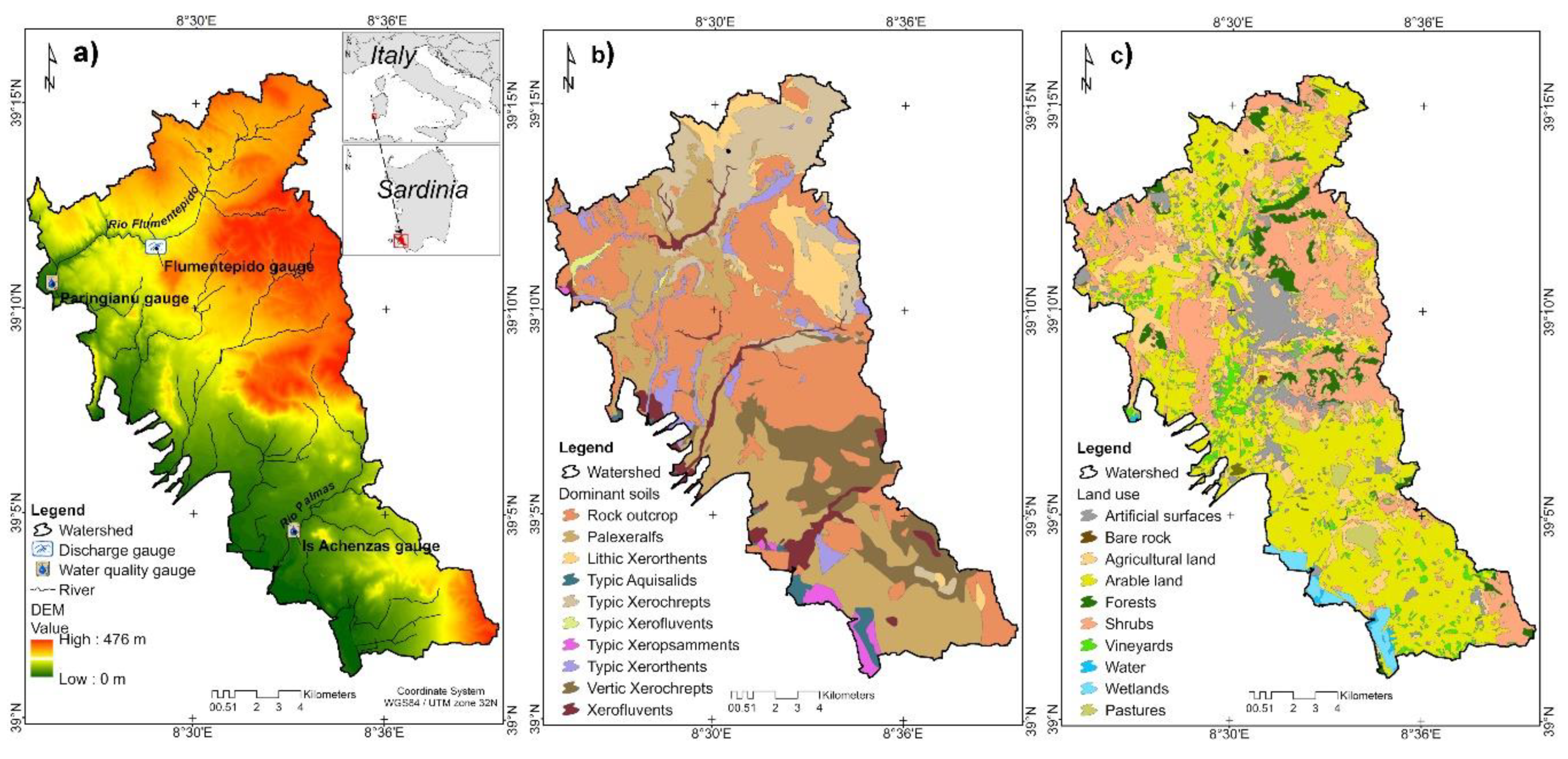
2.1. Study Area

The Sulcis catchment is located in the southwest of Sardinia, Italy (WGS84 UTM32N, 39°10′ north latitude, 8°30′ West longitude, Figure 1) and drains into the Mediterranean Sea. The catchment covers an area of 77 km2, with an elevation ranging from 1 to 475 m above the mean sea level, characterized by a mostly flat and, in some cases gently undulating, terrain [29].
The area is characterized by a Mediterranean semi-arid climate with a bimodal pattern of rainfall distribution (i.e., maximum in the autumn and spring). The mean annual rainfall is 600 mm and the mean annual temperature is 16 °C. The watershed is characterized by an extreme variability of lithological and relief forms and consequently, highly variable soil types, vegetation cover, and land use.
With regards to ecopedological characteristics, the northern part of the basin is characterized by poorly-drained soils with a slow rate of water transmission and high runoff potential. In comparison, the southern part is mainly dominated by well-drained soils with high infiltration rates and high or moderate water transmission. As suggested by De Girolamo and Lo Porto [30] for a surrounding watershed in the south of Sardinia, rainfall patterns exert a strong influence on the hydrological regime, characterized by high flow in autumn and early spring, with extremely low or zero-flow recorded in a river section during the summer months. As a result, water erosion, sediment, and nutrient movement in the soil to the temporary river system towards the watershed outlet follows this seasonal pattern.

2.2. Data Collection and Processing

We used a geospatial dataset available from the Autonomous Region of Sardinia (RAS), including a Digital Elevation Model (DEM), river network, soil map, and land use map. Climate datasets were obtained from the National Centers for Environmental Prediction (NCEP) Climate Forecast System Reanalysis (CFSR) [31]. Furthermore, flow data, sediment, and nutrient parameters were used as independent datasets for performing model calibration and validation. Table 1 provides, for each data type, the scale or resolution, a description, and the data source.

2.2.1. DEM and River Network

A DEM 10 m resolution [32] was used to derive the elevation and slope and delineate watershed and sub-basin division. A detailed examination of the impact of the DEM on SWAT modeling showed that fine resolution data would provide more accurate simulated surface runoff, sediment, and nutrient load at a watershed level [37]. Furthermore, a predefined stream network shapefile was overlaid onto the DEM to improve the extracted geomorphometric terrain characteristics, such as the river network and channel loadings of the associated sub-basin, sub-basin outlets, and other water bodies as ponds or wetlands.

2.2.2. Soil Data

The soil map [33] at a scale of 1:50,000 had 32 map units representing the main soil types of the watershed. According to the United States Department of Agriculture (USDA) Soil Taxonomy Classification [38], Cenozoic soil types characterized by acid effusive rocks (i.e., Typic, Vertic, and Lithic Xerochrepts—Typic and Lithic Xerorthents) dominate the north-central part of the area. Pleistocene soil types characterized by alluvial deposits and eolian sandstones (i.e., Typic, Aquic, and Ultic Palexeralfs—Typic and Calcic Haploreralfs) dominate the central and southern part of the basin, while landscapes on alluvial deposits and conglomerates, eolian deposits, and calcareous crusts of the Holocene (Typic, Vertic, and Aquic Xerofluvents—Typic Xeropsamments) are predominant in the western border or occur as stripes along the main streams (Figure 1b).
Associated soil survey profiles of this dataset were used for deriving information about the physical characteristics of the soil, such as the hydrologic group (i.e., infiltration characteristics); organic carbon content; and silt, sand, and clay contents of soil layers required to parametrize the associated table in the model. Unavailable soil properties, such as the bulk density, saturated hydraulic conductivity, and available water capacity, were estimated with pedotransfer functions in the Soil-Plant-Air-Water model (SPAW) [39] using the soil water tension equations proposed by Saxton and Rawls [40].

2.2.3. Land Use and Agronomic Practices

A land use map at the scale of 1:25,000, with a minimum mapping unit of 0.75 ha and updated in 2008, was used [32]. The dataset was reclassified following the 4th level Corine Land Cover nomenclature [41] in a lookup table with 21 map units. In the northern part, although there is the presence of rainfed farming for the production of durum wheat, rangelands, and pastures, land use is predominantly natural and semi-natural. In contrast, the southern part is predominantly agricultural, with the major crops being horticultural crops in the irrigated district (Figure 1c). Overall, the main land use area includes cereal crops (20%), irrigated crops (26%), rangelands and pasture (19%), and to a lesser extent, vineyards (3.6%) and forest (9%). Detailed agronomic management practices for the main crops were collected to reflect the real application rate of fertilizers and standard crop removal of nutrients in the study area [36]. Cereals are fertilized with 75 kg N ha−1 and 40 kg P ha−1, while vineyards are fertilized with 50 kg N ha−1 and 40 kg P ha−1.

2.2.4. Climate Data

A daily climate dataset at a 0.3125 degrees (~38 km × 38 km) spatial resolution for four weather stations, including the precipitation (mm), minimum and maximum air temperature (°C), solar radiation (MJ m−2), relative humidity (fraction), and wind speed (m s−1), was provided by CFSR due to the inconsistency of local meteorological stations within the study area. The gridded dataset was designed and implemented as a global, high resolution, coupled atmosphere-ocean-land surface-sea ice system, to provide the best estimate of the state of these coupled domains over a given period. The database was completed over the 36-year period from 1979 through 2014 and is available for download for a given location using the interactive web map application [31].

2.2.5. River Discharge Data

Stream river discharge records (m3 s−1) at monthly time steps (period of 1 January 1978 to 31 December 1992) [34] for the Flumentepido gauge station located on the Rio Flumentepido stream (Figure 1a) were used. This gauge station was closed after 1992 and other stream measurements are unavailable for the watershed. As mentioned earlier, the seasonal hydrological records for this gauge confirmed the intermitted regime of the river, with zero-flow recorded during the summer months and an evident rapid rise of peaks in winter months.

2.2.6. Water Quality Data
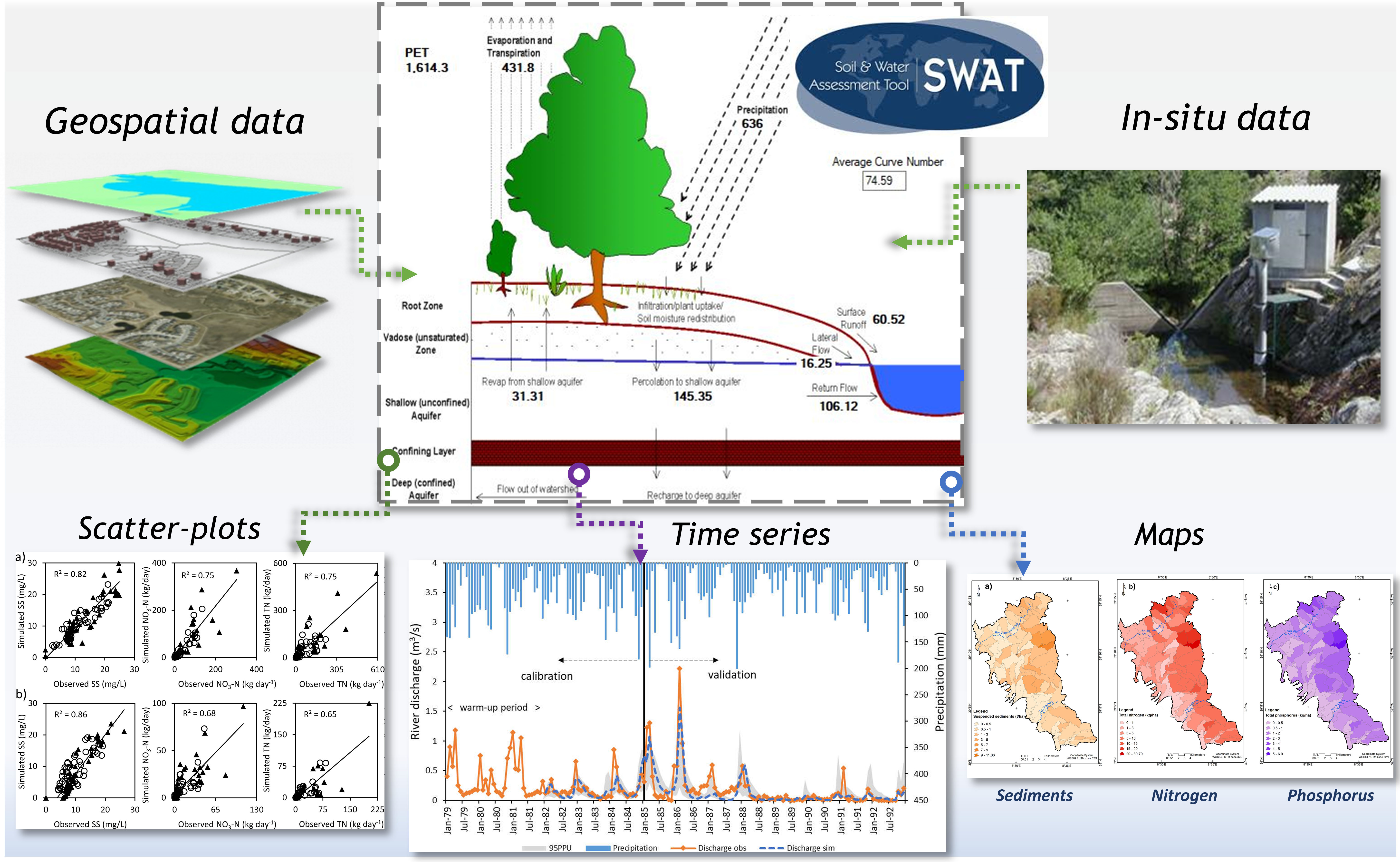
Grab sample concentrations for the period March 2002–December 2009 were available for two gauging stations, located on the “Rio Flumentepido” stream (namely “Paringianu” gauge) and on the “Rio Palmas” stream (namely “Is Achenzas” gauge) (see Figure 1a). The first one is located downstream of the discharge gauge station, representative of complex topographic areas characterized by undulating terrain. Land use contributing to this gauge is 80% natural and semi-natural areas, with extensive agricultural areas, mainly non-irrigated. The second one is representative of areas characterized by flat terrain with intensive irrigated crop farming. Water quality parameters, reported as mg L−1, include suspended sediments (SS), nitrate-nitrogen (NO3-N), total nitrogen (TN), mineral phosphorus (Pmin), and dissolved oxygen (DO), for a total of 70 and 87 samples for Paringianu and Is Achenzas gauges, respectively. This dataset is put together and maintained by the RAS Environmental Protection Agency service (ARPAS) [35] at a monthly time step. Laboratory analyses were performed according to the standard methods proposed by Capri et al. [42] for the examination of water and wastewater, ensuring quality control and assurance procedures of the dataset.

2.3. The SWAT Model

SWAT is a continuous-time, spatially-distributed model used to assess the impact of land use management on the hydrological cycle and material transfer (soil, nutrient, and organic chemical transport and fate) at the watershed scale. SWAT delineated streams, basins, and sub-basins based on DEM. The model divided each basin into hydrological response units (HRU) [43]. Multiple land use-soil-slope options were considered for defining the HRU distribution in each sub-basin, as follows: 10% threshold for land use, 10% for soil, and 10% for slope. Three slope classes were determined, as follows: 0–3%, 3–5%, and >5%. SWAT simulated the hydrologic cycle based on the water balance equation (Equation (1)):
S W t   i = S W 0   i + i = 1 t ( R d a y   i Q s u r f   i E a W s e e p   i Q g w   i ) ,
where SWt i is the final soil water content (mm) on day i, SW0 i is the initial soil water content on day i (mm), t is the time (days), Rday i is the amount of precipitation on day i (mm), Qsurf i is the amount of surface runoff on day i (mm), Ea i is the amount of evapotranspiration on day i (mm), Wseep i is the amount of water entering the vadose zone from the soil profile on day i (mm), and Qgw i is the amount of return flow on day i (mm). The model routed the runoff flows generated by each HRU through the channel network, thereby simulating the watershed. The daily total flow (Qtot i mm) through the channel network was generated by the daily surface flow (Qsurf i mm), lateral flow (Qlatflow i mm), and Qgw i. In this study, the Soil Conservation Service (SCS) curve number method [44] was used to estimate Qsurf i. The curve number method considered the soil infiltration rate, the land cover, the vegetative season, and the antecedent soil moisture condition [45]. The soil erosion was simulated in SWAT with the Modified Universal Soil Loss Equation (MUSLE) [46], while water quality components were simulated with the QUAL2E model [47].

2.3.1. Model Set-Up

The model set-up was implemented using the ArcSWAT 2012 (version 10.21), an ArcGIS-ArcView extension and graphical user interface for SWAT. First, the watershed was delineated and subdivided into 98 sub-basins using the DEM and stream network presented in Table 1. At this stage, two sub-basin outlets were manually added alongside the water quality gauging stations to ensure the comparability of observed and simulated data. Second, multiple HRUs were defined using a threshold of 10-10-10 for the land use, soil, and slope, as optimal criteria to determine the number and type of HRUs in each sub-basin. Third, weather data was inserted in order to generate data tables and create a built-in database required for model configuration and to simulate soil, weather, plant cover, management operations, and urban activities. Fourth, a default plant growth input table was edited to update the application rate for fertilizers. Using dialog boxes, users can edit and personalize the model calibration process with more precise information of the catchment or for a single HRU. Finally, the starting and ending set-up date from January 1979 to December 2009 was defined for running the SWAT simulation procedure. The SWAT auto-irrigation option was adopted for all sub-basins. For more details regarding model theory and set-up, readers are referred to the documentation provided by Arnold et al. [48]. Considering that the SWAT channel output file is expressed as metric tons or kilograms during the time step (i.e., daily, monthly, and annual), the LOAD ESTimator (LOADEST) software developed by the United States Geological Survey [49] was used to generate comparable mean water quality parameters expressed as kilograms per day.

2.3.2. Model Calibration and Validation

Calibration and validation were performed to improve and verify the predictive performances of the model in reproducing the soil-water-atmosphere processes simulated. The model’s evaluation performance was analysed according to the guidelines for carrying out the validation of hydrological models proposed by Biondi et al. [50]. Available records were split into two segments: one was used for calibration (training samples) and the other for validation (test samples). Calibration and validation were carried out at three gauge stations using time series of river discharge and multiple water quality variables measured in the field, in order to capture the spatio-temporal variability within the catchment. Graphical methods were used, including a comparison of the time series, scatter-plots, and spatial maps. Four well-established quantitative statistics [51,52] were computed, namely, the Nash–Sutcliffe Efficiency (NSE), the ratio of the root mean square error (RMSE) to the standard deviation (STDEV) of observed data (RSR), the percent of model bias (PBIAS), and the Kling–Gupta Efficiency (KGE), shown as
NSE = 1 [ i = 1 n ( S i O i ) 2 i = 1 n ( O ¯ O i ) 2 ]
RSR =   RMSE STDEV o b s =   [ i = 1 n ( O i S i ) 2 i = 1 n ( O i   O ^ ) 2 ]
PBIAS = 1 [ i = 1 n ( S i   O i )   ×   100 i = 1 n O i ]
KGE = 1   ( r 1 ) 2 + [ ( σ s σ o ) 1 ] 2 +   [ ( S ^ O ^ ) 1 ] 2 ,
where Si is the simulated data, Oi is the observed data, Ô is the observed mean value, r is the linear correlation coefficient between the simulated and observed variable, σ is the standard deviation (simulated and observed), Ŝ is the simulated mean value, and n equals the number of observations. KGE is a modified version of NSE created to improve the components representing the bias and flow variability [51].
NSE and KGE range from ∞ to 1, with a value closer to 1 producing the most accurate model, while RSR ranges from 0 to large positive values, with a value closer to 0 producing a more accurate model fit [53]. PBIAS values close to 0 produce the most accurate model, while a range ±25% is considered good, with positive values indicating overestimation and negative values indicating model underestimation [54]. Moreover, the 95% prediction uncertainty (95PPU) of the model output variables was calculated to quantify uncertainty ranges [55]. Performance evaluation criteria are based on the rating values proposed by Moriasi et al. [52,53] for watershed-scale models, as follows: very good, good, satisfactory, and not satisfactory model results. Based on the literature, a streamflow simulation is considered satisfactory if NSE > 0.5, RSR ≤ 0.70, and PBIAS < ± 15%; a sediment simulation is considered satisfactory if NSE > 0.45, RSR ≤ 0.70, and PBIAS < ± 20%; and a nutrient simulation is considered satisfactory if NSE > 0.35, RSR ≤ 0.70, and PBIAS < ± 30%. Considering that the KGE metric is mathematically different from NSE and the threshold cannot be simply compared [56], we used this metric as an informative and multi-criterion diagnostic evaluation of the whole model.
The SWAT-CUP 2012 software was used following the protocol suggested by Abbaspour et al. [57] for successful calibration and uncertainty analysis, by implementing the Sequential Uncertainty Fitting procedure (SUFI-2). SUFI-2 is an iterative and optimization algorithm employed to fit a set of best parameter ranges and compute a threshold assigned to different objective functions available in the software.
For river discharge at Flumentepido gauge, the starting and ending date was constrained by the common period of the dataset available for the watershed. Therefore, the period “1982–1985” was set for model calibration, the period “1986–1992” was set for validation, and the period “1979–1981” was set for the initial SWAT model warm-up. Firstly, the selected model parameters affecting the discharge simulation process were inserted within SWAT-CUP calibration. Published studies of similar catchments were identified to establish initial range values plausible for the study area and Mediterranean climate conditions [2,4,58,59]. As indicated by De Girolamo and Lo Porto [30], we assumed a transposition of the groundwater parameters, soil parameters, and management parameters for the same combination of input data. Secondly, a sensitivity analysis and manual trial-and-error procedure was performed to identify the most relevant parameters to be optimized, deleting the non-sensitive ones. Thirdly, the model ran the first iteration with at least 500 simulations, updating new parameter ranges after each iteration and executing up to five iterations until attaining reasonable objective function results. Finally, discharge validation was performed by inserting test samples and updating the time-lap. Once the streamflow calibration was completed for the whole basin, the focus turned to sediment and nutrient representation. For the water quality at gauge stations, calibration was set to the period “2002–2005”, while validation was performed for the period “2006–2009”, following the same procedure explained above. For more details regarding SUFI-2 software capabilities and details of method implementation, readers are referred to literature on the subject [57,60].

3. Results and Discussion

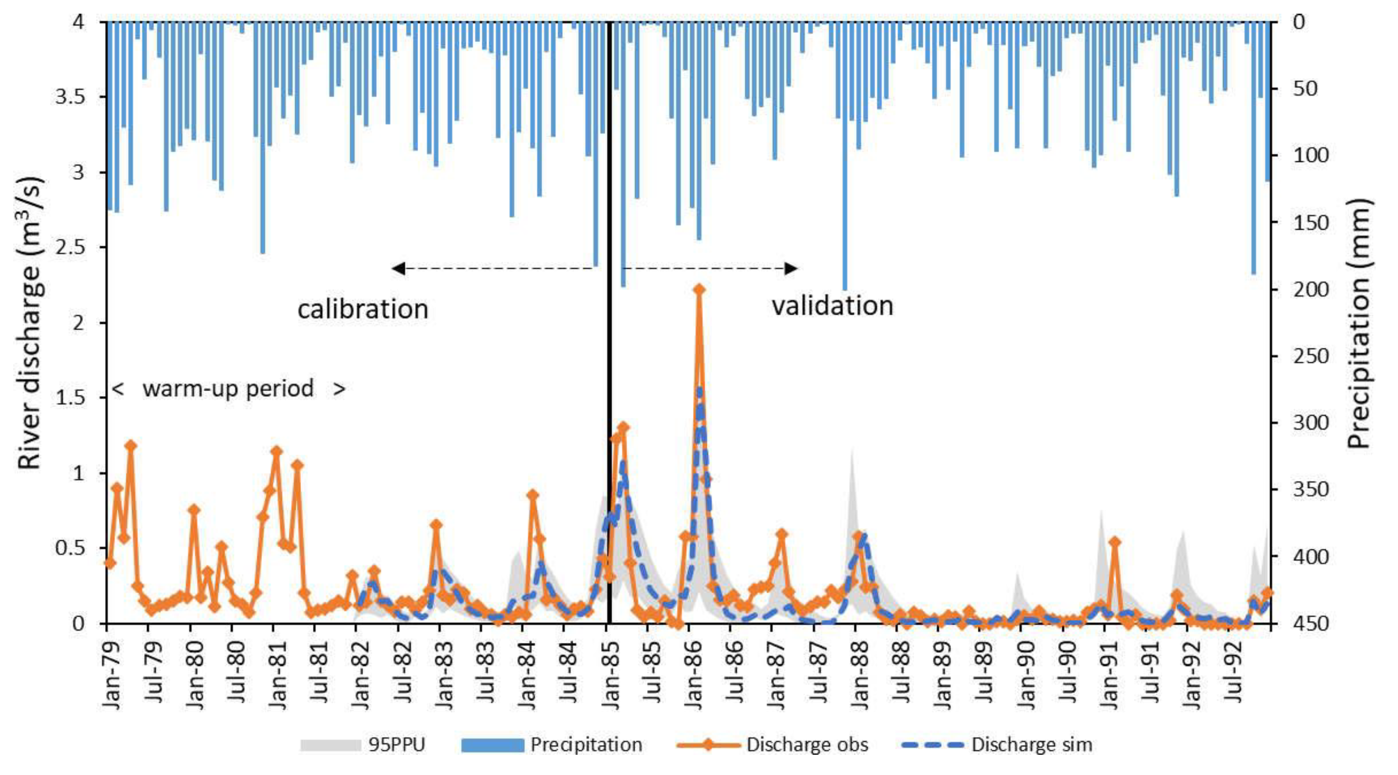
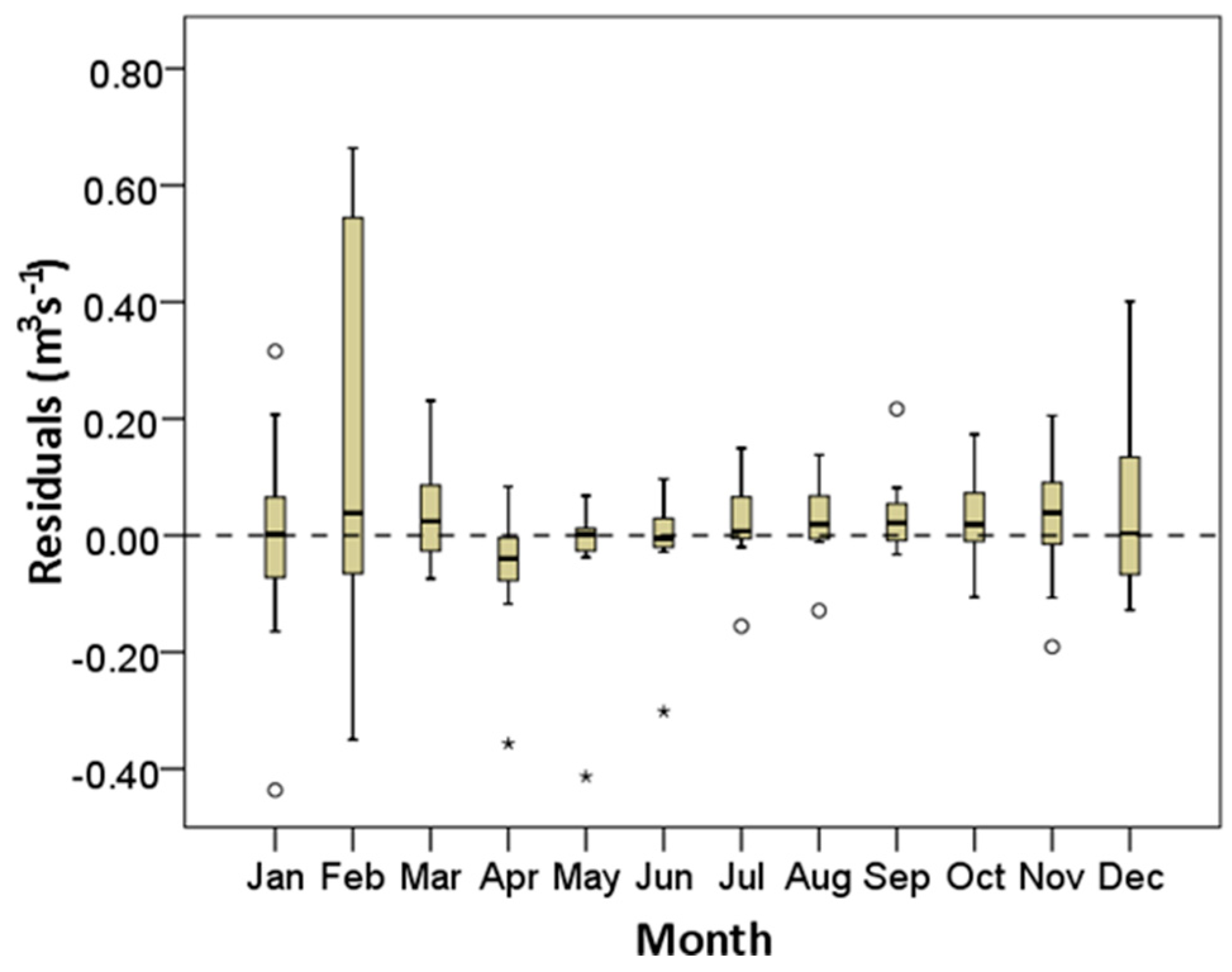
3.1. Calibration and Validation

Descriptive statistics of performance measures for streamflow and water quality at the monitoring stations during calibration and validation are reported in Table 2. Graphs of long-term evolution and scatter-plots showing the relationship between observed and simulated data are depicted in the following figures.

3.1.1. Streamflow Calibration and Validation

The goodness-of-fit objective function results of model calibration and validation for river streamflow at Flumentepido gauge suggest that the model can adequately reproduce the hydrological processes in the watershed (Table 2). For the calibration period, the NSE was 0.5 (satisfactory), the RSR was 0.71 (unsatisfactory), the PBIAS was 2.2% (very good), and the KGE was 0.69. For the validation period, the NSE was 0.70 (satisfactory), the RSR was 0.55 (good), the PBIAS was 18.7% (unsatisfactory), and the KGE was 0.6. Overall, the performance measures suggest that the model configuration better performs river discharge during validation than calibration, with higher NSE and RSR performance statistics. The increase of PBIAS and slight decrease of KGE metrics indicate a weakness of the model in terms of correctly simulating some peak flows and low flows, although the PBIAS value is <±30%, which is the maximum acceptable model performance for streamflow [52]. Underestimations can be seen in Figure 2, when moderate rainfall events occurred (e.g., February 1987 and 1991), while intense rainfall events (e.g., January–February 1986) corresponded to a well-plotted peak between observed and simulated lines.
The analysis of residuals errors (Figure 3) calculated as differences between the measured and simulated values confirmed that there are seasonality effects for peak flows. Streamflow is underestimated by the model, as indicated by the predominance of positive residuals during winter months, while it is less frequently overestimated or quite well-estimated during the summer. The underestimation of major peak flow events was reported in the literature for arid and semi-arid watersheds and ephemeral streams [61,62] and could be explained by bias in the meteorological data not spatially well-distributed, or more general errors in data inputs [63]. Nevertheless, uncertainties associated with river streamflow can be seen in Figure 2 when looking at the 95PPU range that generally well-bracketed the simulation line and confirming the model performance, as well as the quite large uncertainty interval in terms of some peak flow.

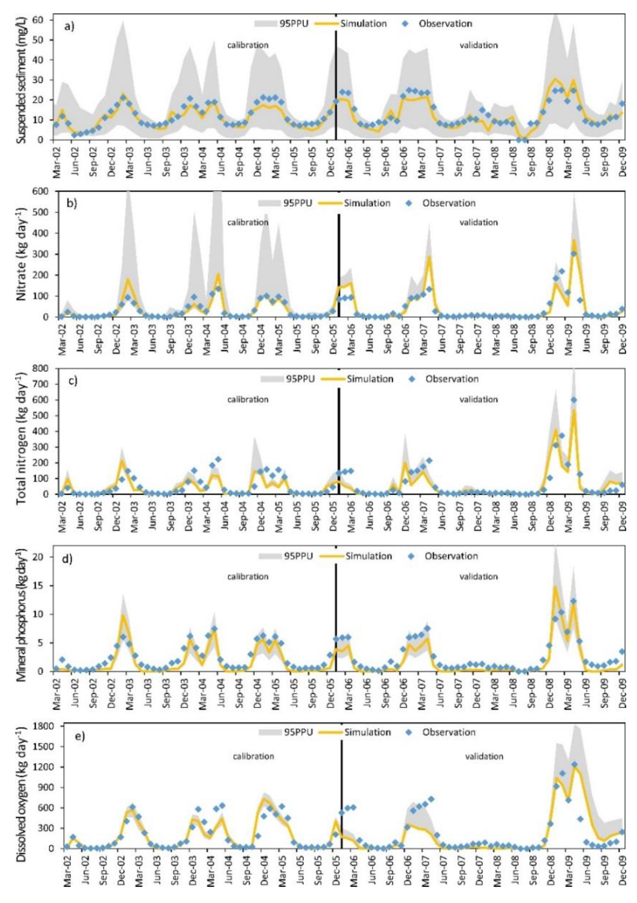
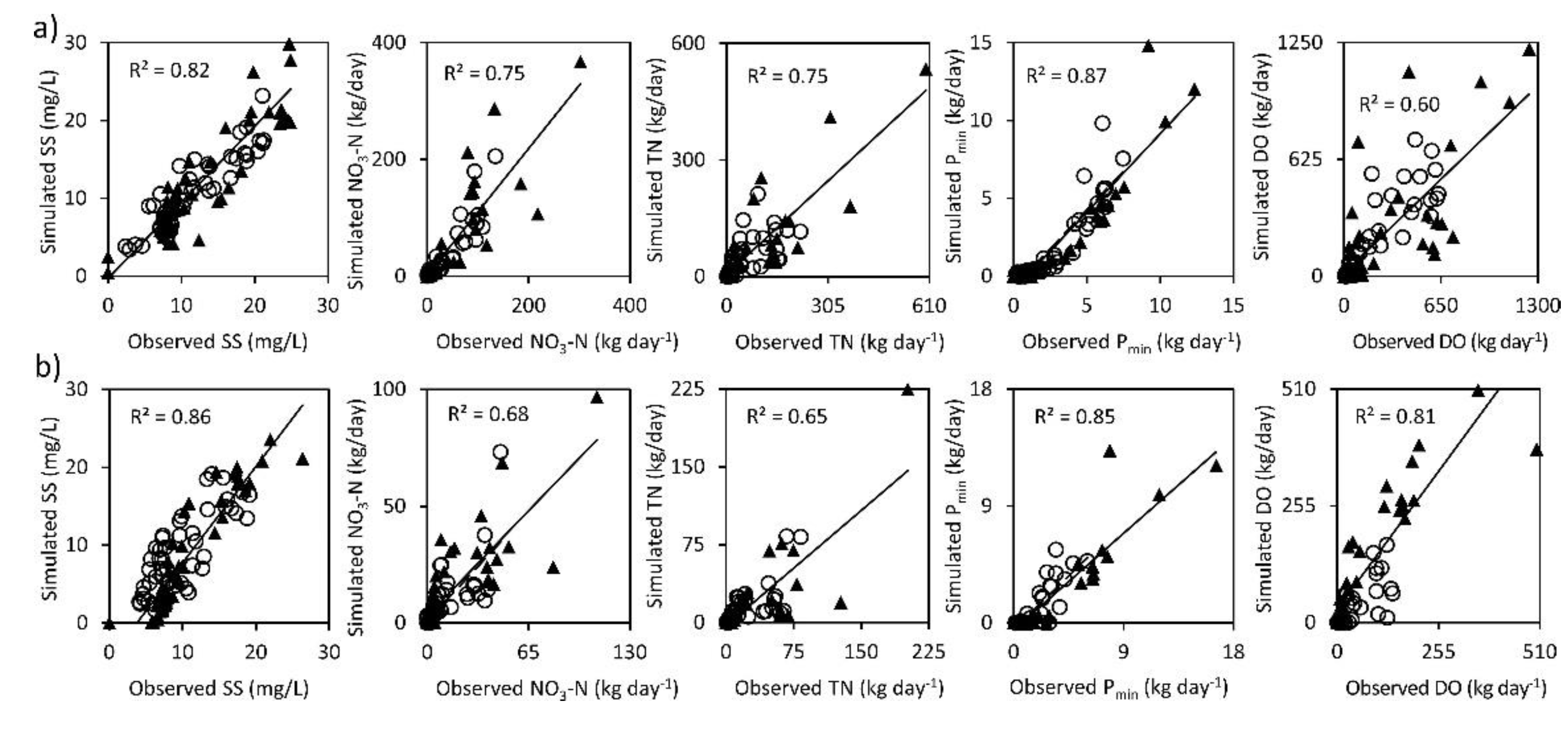
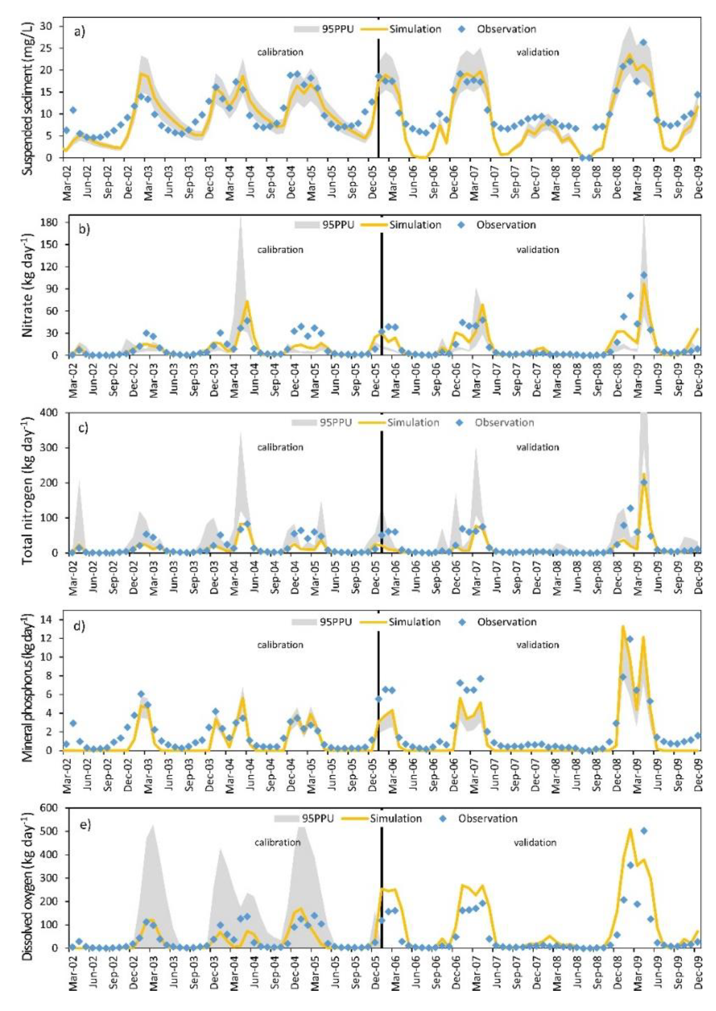
3.1.2. Water Quality Calibration and Validation

The simulation results for Paringianu and Is Achenzas gauging stations suggest that the model can adequately reproduce water quality parameters and their spatio-temporal evolution in the watershed. At Paringianu gauge (Table 2), the statistical goodness-of-fit objective function NSE for SS was 0.81 (very good) for calibration and 0.78 (good) for validation. Interestingly, the RSR and PBIAS values for SS during calibration and validation corresponded to “very good” performance evaluation criteria, <±10%, while KGE was 0.87 during validation. The NSE values for NO3-N were 0.71 (very good) during calibration and 0.60 (good) during validation, and the RSR and PBIAS values corresponded to “satisfactory” and “very good” ratings during validation, while the final KGE value was 0.69. The model results for TN showed a performance rating of “very good” for NSE during validation, with a value of 0.74; a PBIAS value of 13.2%, and a KGE value that reached 0.79. Similarly, Pmin model performance ratings were “very good”, with an NSE value of 0.76 and RSR value of 0.49, but with an unexpected “not satisfactory” PBIAS value of 32.2%. The NSE, RSR, and PBIAS values for DO were “very good” during calibration, while the model’s performance during validation was “good” for NSE and PBIAS and “satisfactory” for RSR, and the KGE was 0.73. The temporal results for monthly observed and simulated water quality loads at Paringianu gauge during calibration and validation are shown in Figure 4. The graphical evaluation of SS concentrations reveals a good trend between observed and simulated lines and consequently, the model’s ability to predict peaks and recession curves.
Uncertainties associated with SS plotted as the 95PPU range envelop most of the observations with a large thickness. The scatter-plots in Figure 5a show the relationship between observed and simulated monthly water quality. Model simulation predictions for SS at Paringianu gauge demonstrate a high coefficient of determination with observed data, while the straight line for validation data indicates a very good fit with the 1:1 line. The temporal trend in Figure 4 for NO3-N confirmed performance values during calibration, while during model validation, overestimation occurred during February and March 2006 and April 2007. On the contrary, while the TN graph simulation did not capture peak events well during calibration, the validation plots showed a more regular trend, although the underestimation of peaks was evident. The scatter-plot confirmed that the observed versus simulated data straight-line did not fit very well with the 1:1 best fit line.
Overall, the SWAT model successfully simulated NO3-N and TN in the watershed, despite the poor performance when simulating specific peaks, which could be attributed to the inadequate simulation of processes and pathways for all reactive nitrogen, including environmental and in-stream processes. Previous studies reported that the SWAT model tends to underestimate peaks in discharge and consequently underestimates nitrate loads [64].
It is well-known that sediment and chemical fluxes are controlled by river regimes and discharge [65]. Therefore, it is fundamental to improve the accuracy of the water flow model and specific narrow-peaks. Moreover, Zeiger and Hubbart [66] highlighted the need to deeply improve the loading algorithms and routines of all nitrogen pools (i.e., ammonium and nitrite) in SWAT simulations because these are generally underestimated. Similar to the nitrogen pool, the temporal trend for Pmin showed peaks that were underestimated during validation and the 95PPU range did not capture all uncertainty, and in fact, most of the data points in Figure 5a are below the straight line. Finally, DO displayed a better temporal trend during calibration, while during the validation period, there was an underestimation of some peaks. Figure 5a confirms the poor coefficient of determination for validation data, with the straight line being under the 1:1 line.
At Is Achenzas gauge station (Table 2), the statistical goodness-of-fit objective function NSE for SS was 0.42 (not satisfactory) for calibration and 0.55 (satisfactory) for validation. Similarly, the RSR value for SS during calibration and validation moved from “not satisfactory” to “satisfactory” performance evaluation criteria, while PBIAS was 19% and KGE was 0.61. The NSE values for NO3-N were 0.47 (satisfactory) during calibration and 0.67 (good) during validation, the RSR and PBIAS values corresponded to “good” and “very good” ratings during validation, and the final KGE value was 0.74. The model results for TN showed an NSE value 0.58 (good) during validation and RSR value of 0.65 (satisfactory), while PBIAS during calibration and validation was “satisfactory”.
Interestingly, the Pmin model performance rating for NSE moved from “satisfactory” to “very good” during validation and the KGE value increased to 0.59, although the final PBIAS value was 38.5% (not satisfactory). Contrasting results were obtained for DO, with the NSE value of 0.55 being obtained during validation (good), RSR value of “satisfactory”, and KGE value of 0.42. It should be noted that SWAT-CUP was not able to carry out the DO validation procedure, so performance values were calculated using a spreadsheet.
The temporal results of observed and simulated water quality concentrations at Is Achenzas gauge in Figure 6 graphically confirm some contrasting results obtained when calculating goodness-of-fit objective function values. The graphical plot of SS concentrations reveals that simulation generally underpredicted summer concentrations, while peak concentrations were well-captured. Similarly, the 95PPU range does not envelop the underprediction line very well, while peaks are well-captured.
The scatter-plots in Figure 5b show a good coefficient of determination for SS, but also underpredicted points during validation below the straight line. A visual inspection of the temporal trend in Figure 6 for NO3-N and TN showed a similar trend, with underestimations for specific peaks during calibration and validation, while low concentrations during summer are generally well-recognized.
Furthermore, the scatter-plot for NO3-N and TN confirmed that straight lines do not fit the 1:1 best fit line very well. As reported for the Paringianu gauge, it is possible to hypothesize that the poor performance of the peak simulation could be attributed to bias in the simulation. Nevertheless, Is Achenzas gauge is located in an intensive agricultural area, so it is challenging to correctly simulate the nitrogen cascade and transfer from agricultural soils to the drainage network. In this sense, previous studies have reported that hot-spot areas of nitrogen surplus attributed to input uncertainty (e.g., fertilizers, manure, and point sources) greatly altered the nitrogen budget and leaching [67].
At Is Achenzas gauge, the temporal trend for Pmin peaks was underestimated during validation and the 95PPU range did not capture all uncertainty, while most of the validation points in the scatter-plot in Figure 5b are below the straight line. On the contrary, the DO concentration showed a better temporal trend during calibration, while overestimation is depicted during the validation period (e.g., winter months 2005–2006). Figure 5b confirms the overestimation, with validation points above the straight line. Nonetheless, all values of the coefficient of determination were satisfactory for the validation period.

3.1.3. Sensitive Parameters

Table 3 reports a total of 27 of the most sensitive parameters identified with SWAT-CUP for calibrating the model, including their descriptions, unit, and final range values. The following parameters are the most sensitive to water flow: the baseflow recession constant (ALPHA_BF), runoff curve number (CN2), soil evaporation compensation factor (ESCO), groundwater delay time (GW_DELAY), groundwater re-evaporation coefficient (GW_REVAP), threshold depth of water in the shallow aquifer required for return flow to occur (GWQMIN), and deep aquifer percolation fraction (RCHRG_DP); the following for sediments: the linear parameter for channel sediment routing (SPCON), exponent parameter for channel sediment routing (SPEXP), channel erodibility factor (CH_COV1), channel cover factor (CH_COV2), USLE soil erodibility factor (USLE_K), and sediment concentration in lateral and groundwater flow (LAT_SED); the following for nitrate: the nitrate percolation coefficient (NPERCO), initial concentration of nitrate in the shallow aquifer (SHALLST_N), concentration of nitrogen in rainfall (RCN), nitrogen uptake distribution parameter (N_UPDIS), and organic nitrogen enrichment ratio (ERORGN); the following for total nitrogen: the organic nitrogen in the baseflow (LAT_ORG), rate constant for the hydrolysis of organic nitrogen to ammonia in the reach (BC3), and rate coefficient for organic nitrogen settling in the reach at 20 °C (RS4); the following for mineral phosphorus: the rate constant for the decay of organic phosphorus to dissolved phosphorus (BC4), phosphorus availability index (PSP), phosphorus soil partitioning coefficient (PHOSKD), phosphorus percolation coefficient (PPERCO), and soluble phosphorus concentration in groundwater loading (GWSOLP); and the following for dissolved oxygen: temperature adjustment factor (TMPINC). Overall, these parameters govern the system inputs, storage, movement of surface or subsurface water, and system outflows into HRUs.
As previously described, initial range values from published studies of Mediterranean climates were utilized because the model was very sensitive and out-of-range realistic values can give insufficient results. In fact, as SUFI-2 is an iterative algorithm, calibration starts in the first iteration by assuming a large uncertainty [55], while in the last iteration, a single parameter was fitted and fixed. Overall, considering that the model is a simplification of complex dynamics and processes in the watershed, the reported sensitive parameters are those that best represent all sources of uncertainties (i.e., best estimates for this model, variables, and data used) and model assumptions governed by model equations that describe water flow and hydrological processes.

3.2. Water Balance

The average monthly water balance components over the simulation period are reported in Table 4. The results showed that evapotranspiration is the predominant outflow component, with 431 mm year−1, accounting for approximately 68% of the annual precipitation (635 mm), while about 30% was the water yield, namely water discharged in the channels. As shown in Table 4, the surface runoff is 60.5 mm year−1, representing about 9.5% of the annual precipitation, confirming that this outflow component that governed soil erosion is not significant at a watershed level. The monthly surface runoff has significant seasonal peaks during winter months, following the Mediterranean precipitation pattern [58], with associated sediment and pollutant losses, as depicted in Figure 4 and Figure 6.
On the contrary, the transition to an ephemeral state of most river corridors gave negligible water yield values during summer month. The potential evapotranspiration was equal to 1614 mm year−1, with a peak during summer months of up to 7.9 mm day−1. These results are in agreement with those obtained by De Girolamo and Lo Porto [30] in the Rio Mannu basin and confirmed the overall reliability of the model.

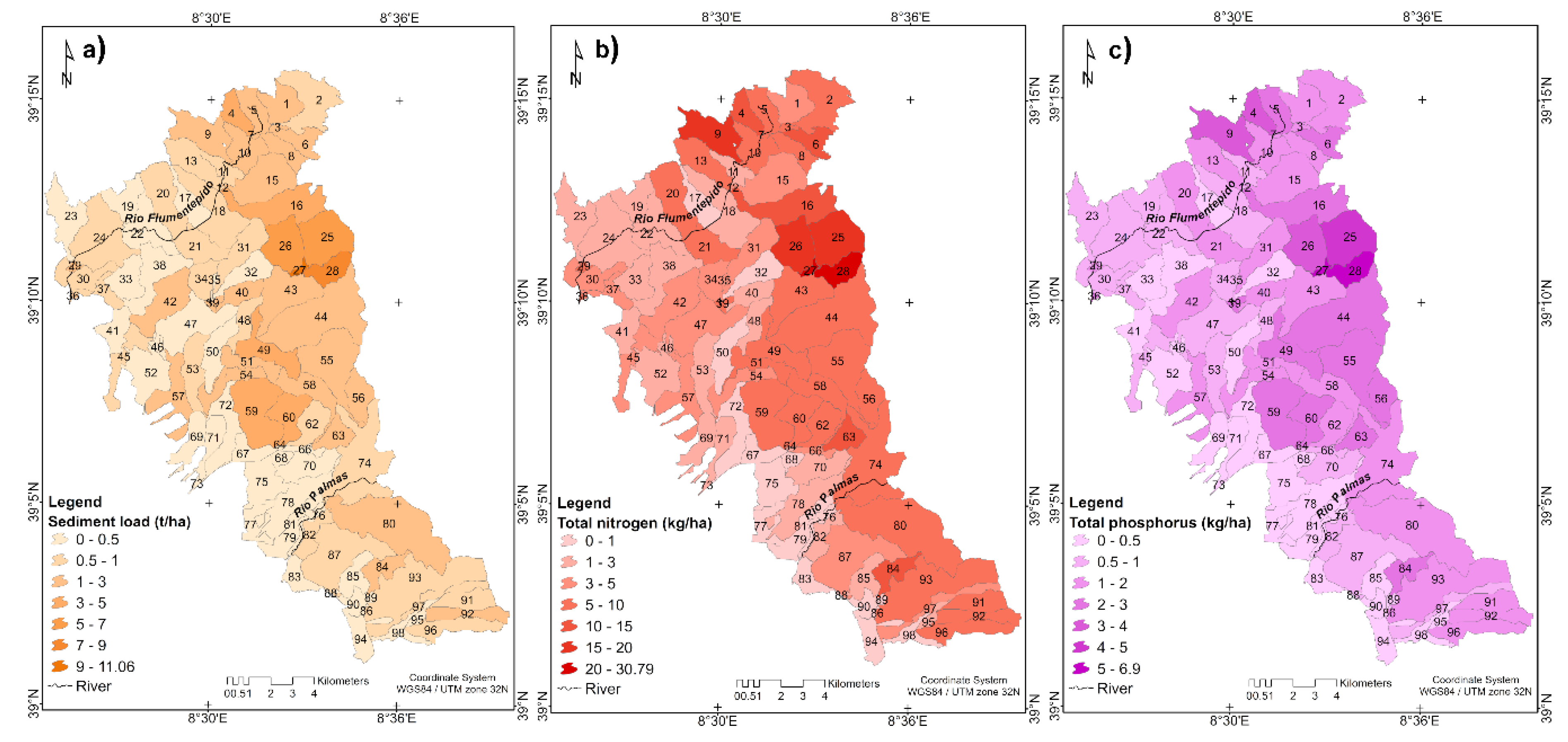
3.3. Water Quality and High Loading Areas

The 28-year (1982–2009) annual average SWAT model outputs for sediment load, TN, and total phosphorus (TP) loadings were calculated at a sub-basin and watershed level to provide insights regarding ongoing environmental pressures (Table 5). Overall, at a watershed level, the simulated average load of sediments was 1.13 t ha−1 year−1. Regarding land use, the loading rate was 0.97 t ha−1 year−1 for durum wheat, 3.66 t ha−1 year−1 for pasture, 1.52 t ha−1 year−1 for tall shrublands, 0.32 t ha−1 year−1 for eucalyptus plantation, and 0.05 t ha−1 year−1 for evergreen forest.
The annual average sediment load predicted is lower than both the threshold limit of tolerable soil erosion in Europe (1.40 t ha−1 year−1) [68], and the soil loss rate for the Mediterranean climatic zone (4.61 t ha−1 year−1) [69]. Overall, these results are comparable to those from studies performed in the Mediterranean area using the SWAT model. For instance, Nerantzaki et al. [70] reported a mean erosion rate of 0.97 t ha−1 year−1 in a karstic watershed in Greece. Similarly, Gamvroudis et al. [2] found an average sediment yield equal to 0.85 t ha−1 year−1 in a large temporary river basin in Greece. Conversely, in a recent study in the Carapelle watershed with temporary rivers (Apulia, Italy), Ricci et al. [4] reported an average annual sediment load of 6.8 t ha−1 year−1. Nevertheless, this river basin has steep-slope areas with high erosion rates (up to 13 t ha−1 year−1), while on the alluvial plain, the sediment yield was comparable to that of the present study (<1 t ha−1 year−1). At the watershed level, the obtained nutrient loads estimation was 4.85 kg ha−1 year−1 for TN and 1.18 kg ha−1 year−1 for TP. Considering differences in watershed characteristics between areas, these values seem to be consistent with those obtained in the Mediterranean area. For instance, De Girolamo et al. [71], for the conterminous Rio Mannu basin in southern Sardinia, reported an average of 0.86 kg ha−1 year−1 for TP. Similarly, a recent nutrient apportionment tool tested in south-eastern Italy showed that the average TN riverine export was 2.8 and 5.2 kg ha−1 year−1 at a basin scale and for productive lands, respectively [72]. The authors attributed the relatively low rates of TN losses in the watershed to the fact that groundwater was the principal receptor of the NO3-N leached from fractured soils. These results reflect those of Carvalho-Santos et al. [73], who reported, for the baseline scenario in a medium-sized Mediterranean watershed in Portugal, values of 1.04 kg ha−1 year−1 and 1.09 kg ha−1 year−1 for TN and TP, respectively.
In another study in a medium-sized Greek catchment, Panagopoulos et al. [58] found that the mean annual TN yield was 20 kg ha−1 year−1. Although this result differs from the findings presented here, this discrepancy could be attributed to the large watershed (405 km2) with a very high slope gradient and higher sediment yield (14 t ha−1 year−1). Overall, these regional studies further confirm the importance of local land uses and management of determining in-stream water erosion and the consequent sub-basin load across the catchment. Spatialized water quality loads were calculated from the SWAT model for each sub-basin’s outlet. Figure 7 shows the average annual loads for sediment load, TN, and total TP during the period 1982–2009.
These maps are quite revealing and interesting in several ways, showing differences, especially in the northern part of the watershed, where some sub-basins (e.g., 9, 27, and 28) have a high rate of sediment (up to 11 t ha−1 year−1), TN (up to 30 kg ha−1 year−1), and TP (up to 6.9 kg ha−1 year−1) exports. These results corroborate our earlier hypothesis that poorly-drained soils in the northern portion of the basin are more prone to erosion, while well-drained soils with gentle slopes in the southern part are less prone to surface runoff, sediment erosion, and nutrient leaching. Similarly, previous studies have reported a strong relationship between geomorphological and pedological characteristics of the basin and related soil-based hydrological processes [4,74,75]. In this sense, it is interesting to note that areas with higher sediment load transport are the same, with the highest nutrient leaching, confirming that these nutrients and fluxes are strictly related to the sediment load transported through the river network [76].
Moreover, the maps reveal that some sub-basins in the southern watershed (e.g., 63 and 84) have hot-spot areas contributing up to 1.29 t ha−1 year−1, 12 kg ha−1 year−1, and 2.4 kg ha−1 year−1 for sediment load, TN, and TP, respectively. These results may be explained by the fact that in these sub-basins, intensive agricultural practices and fertilization are more frequent, and consequently, these generate relatively higher nutrient loads. However, a possible source of uncertainty is due to the role of agricultural ditches (vegetated and unvegetated) in nitrogen retention (i.e., in-ditch denitrification), as suggested by Soana et al. [77] for NO3-N pollution removal by the ditch network. This study reveals that vegetated ditches intercept and decrease nitrogen loads in surface waters generated in the surrounding agricultural lands. This view is supported by Lassaletta et al. [78], who confirmed that nitrogen retention in the Mediterranean catchments is high compared to nitrogen inputs.
These findings raise important implications for developing future best management and soil conservation practices prior to promoting land use scenarios in the area, as stated in the introduction. In accordance with extensive recent studies, allocating second-generation lignocellulosic crops in fragile and degradation prone areas could mitigate environmental risks associated with the agronomic management enhancing ecosystem services [79]. Future studies on the current topic should be undertaken to investigate simulations with climate and land use scenarios and management approaches with suitable bioenergy crops for promoting environmental sustainability and profitability for farmers in the study area. Further work needs to be done to establish whether scenarios with bioenergy crops result in changes in the water balance, as suggested by other studies [80,81].
Even though large and detailed datasets were used to ensure that reliable and consistent results were obtained, their generalizability is subject to certain limitations. First, the river discharge data is dated and limited to one gauge station. It is worth noting that changes in the precipitation pattern or inter-annual variability affect stream flow and consequently the amplitude of soil erosion and nutrient export. Second, uncertainty also stems from the water quality data collected at monthly time steps. An automatic grab sample concentration collected at daily or sub-daily time steps would ensure lower uncertainty in the results. Third, another weakness was the paucity of data regarding land use and site-specific management practices. Detailed data on agronomic management (i.e., tillage, fertilizer application, and irrigation) would further improve model calibration. Finally, further work should be conducted to improve model simulations, incorporating other biophysical parameters using remote sensing and GIS data and improved dynamic routing algorithms for nitrogen and phosphorus pools, as well as for bioenergy crops.

4. Conclusions

The SWAT model was calibrated and validated using detailed grab sample data collected by three gauge stations located in the southwest of Sardinia, Italy. The SUFI-2 sequential uncertainty fitting algorithm was used to parametrize the model and calculate the objective function for monthly discharge, suspended sediment, nitrate nitrogen, total nitrogen, mineral phosphorus, and dissolved oxygen. This study has shown that the model reliably represented the spatiotemporal variability of the flow regime, sediments, and nutrient fluxes in the ephemeral river system. Water balance simulations revealed that evapotranspiration is a dominant outflow component, while surface runoff is a key component during winter months because most of the river channels are dry during summer months. The results obtained show that sediment loss is lower than both the threshold limit of tolerable soil erosion in Europe and the soil loss rate for the Mediterranean drylands. Nevertheless, the research has shown that the catchment has hotspot areas of sediment and nutrient loadings in the north-east and southern part of the basin. The evidence from this study indicates that high erosion rates and nutrient removal were generally associated with steep-slope areas and arable crops, as suggested by previous studies of the Mediterranean area. The outcomes of this study establish a quantitative framework to assess the impact of anthropogenic pressures on the hydrological response of a river basin with an intermittent flow and provide a basis for implementing new agronomic scenarios to meet production and environmental goals in future targeting studies.

Author Contributions

Conceptualization, G.P.; Data curation, G.P.; Formal analysis, G.P. and M.C.; Funding acquisition, G.B.; Investigation, G.P.; Methodology, G.P. and M.N.; Project administration, G.B.; Software, G.P.; Supervision, G.P., G.B., M.C., F.L. and F.A.; Validation, G.P.; Visualization, G.P., L.T. and F.L.; Writing—original draft, G.P., G.B., M.C., L.T., F.L., F.A., A.D.M. and M.N.; Writing—review & editing, G.P., G.B., M.C., L.T., F.L., F.A., A.D.M. and M.N. All authors have read and agreed to the published version of the manuscript.

Funding

This research received no external funding.

Acknowledgments

The authors gratefully thank Rita Puddu, Stefania Fanni, and Alessandro Marrone from the Agricultural Research Agency of Sardinia (AGRIS) for having provided the pedological map and soil profile data set for the study area that have been used in this work.

Conflicts of Interest

The authors declare no conflicts of interest.

References

  1. Cammalleri, C.; Barbosa, P.; Micale, F.; Vogt, J.V. Climate Change Impacts and Adaptation in Europe, Focusing on Extremes and Adaptation until the 2030s. PESETA-3 Project, Final Sector Report on Task 9: Droughts; JRC European Commission: Ispra, Italy, 2017. [Google Scholar]
  2. Gamvroudis, C.; Nikolaidis, N.P.; Tzoraki, O.; Papadoulakis, V.; Karalemas, N. Water and sediment transport modeling of a large temporary river basin in Greece. Sci. Total Environ. 2015, 508, 354–365. [Google Scholar] [CrossRef]
  3. De Girolamo, A.M.; Bouraoui, F.; Buffagni, A.; Pappagallo, G.; Lo Porto, A. Hydrology under climate change in a temporary river system: Potential impact on water balance and flow regime. River Res. Appl. 2017, 33, 1219–1232. [Google Scholar] [CrossRef]
  4. Ricci, G.F.; De Girolamo, A.M.; Abdelwahab, O.M.M.; Gentile, F. Identifying sediment source areas in a Mediterranean watershed using the SWAT model. Land Degrad. Dev. 2018, 29, 1233–1248. [Google Scholar] [CrossRef]
  5. Serpa, D.; Nunes, J.P.; Santos, J.; Sampaio, E.; Jacinto, R.; Veiga, S.; Lima, J.C.; Moreira, M.; Corte-Real, J.; Keizer, J.J.; et al. Impacts of climate and land use changes on the hydrological and erosion processes of two contrasting Mediterranean catchments. Sci. Total Environ. 2015, 538, 64–77. [Google Scholar] [CrossRef] [PubMed] [Green Version]
  6. Sorando, R.; Comín, F.A.; Jiménez, J.J.; Sánchez-Pérez, J.M.; Sauvage, S. Water resources and nitrate discharges in relation to agricultural land uses in an intensively irrigated watershed. Sci. Total Environ. 2019, 659, 1293–1306. [Google Scholar] [CrossRef] [PubMed]
  7. Vermeulen, S.J.; Challinor, A.J.; Thornton, P.K.; Campbell, B.M.; Eriyagama, N.; Vervoort, J.M.; Kinyangi, J.; Jarvis, A.; Läderach, P.; Ramirez-Villegas, J.; et al. Addressing uncertainty in adaptation planning for agriculture. Proc. Natl. Acad. Sci. USA 2013, 110, 8357–8362. [Google Scholar] [CrossRef] [Green Version]
  8. Fava, F.; Pulighe, G.; Monteiro, A.T. Mapping Changes in Land Cover Composition and Pattern for Comparing Mediterranean Rangeland Restoration Alternatives. Land Degrad. Dev. 2016, 27, 671–681. [Google Scholar] [CrossRef]
  9. Raclot, D.; Le Bissonnais, Y.; Annabi, M.; Sabir, M.; Smetanova, A. Main Issues for Preserving Mediterranean Soil Resources From Water Erosion Under Global Change. Land Degrad. Dev. 2018, 29, 789–799. [Google Scholar] [CrossRef]
  10. Veldkamp, T.I.E.; Wada, Y.; de Moel, H.; Kummu, M.; Eisner, S.; Aerts, J.C.J.H.; Ward, P.J. Changing mechanism of global water scarcity events: Impacts of socioeconomic changes and inter-annual hydro-climatic variability. Glob. Environ. Chang. 2015, 32, 18–29. [Google Scholar] [CrossRef]
  11. Wolf, J.; Kanellopoulos, A.; Kros, J.; Webber, H.; Zhao, G.; Britz, W.; Reinds, G.J.; Ewert, F.; de Vries, W. Combined analysis of climate, technological and price changes on future arable farming systems in Europe. Agric. Syst. 2015, 140, 56–73. [Google Scholar] [CrossRef]
  12. Ponti, L.; Gutierrez, A.P.; Ruti, P.M.; Dell’Aquila, A. Fine-scale ecological and economic assessment of climate change on olive in the Mediterranean Basin reveals winners and losers. Proc. Natl. Acad. Sci. USA 2014, 111, 5598–5603. [Google Scholar] [CrossRef] [Green Version]
  13. Hussain, M.I.; Muscolo, A.; Farooq, M.; Ahmad, W. Sustainable use and management of non-conventional water resources for rehabilitation of marginal lands in arid and semiarid environments. Agric. Water Manag. 2019, 221, 462–476. [Google Scholar] [CrossRef]
  14. Dauber, J.; Miyake, S. To integrate or to segregate food crop and energy crop cultivation at the landscape scale? Perspectives on biodiversity conservation in agriculture in Europe. Energy Sustain. Soc. 2016, 6, 25. [Google Scholar] [CrossRef] [Green Version]
  15. Soldatos, P. Economic Aspects of Bioenergy Production from Perennial Grasses in Marginal Lands of South Europe. Bioenergy Res. 2015, 8, 1562–1573. [Google Scholar] [CrossRef]
  16. Anderson-Teixeira, K.J.; Duval, B.D.; Long, S.P.; DeLucia, E.H. Biofuels on the landscape: Is “land sharing” preferable to “land sparing”? Ecol. Appl. 2012, 22, 2035–2048. [Google Scholar] [CrossRef] [Green Version]
  17. The Global Bioenergy Partnership (GBEP). Available online: http://www.globalbioenergy.org (accessed on 30 September 2019).
  18. Alexopoulou, E.; Zanetti, F.; Scordia, D.; Zegada-Lizarazu, W.; Christou, M.; Testa, G.; Cosentino, S.L.; Monti, A. Long-Term Yields of Switchgrass, Giant Reed, and Miscanthus in the Mediterranean Basin. BioEnergy Res. 2015, 8, 1492–1499. [Google Scholar] [CrossRef]
  19. Testa, R.; Foderà, M.; Maria, A.; Trapani, D.; Tudisca, S.; Sgroi, F. Giant reed as energy crop for Southern Italy: An economic feasibility study. Renew. Sustain. Energy Rev. 2016, 58, 558–564. [Google Scholar] [CrossRef]
  20. European Commission. Proposal for a DIRECTIVE OF THE EUROPEAN PARLIAMENT AND OF THE COUNCIL on the Promotion of the Use of Energy from Renewable Sources (Recast). COM/2016/0767 Final/2—2016/0382 (COD); European Commission: Bruxelles, Belgium, 2017. [Google Scholar]
  21. Pulighe, G.; Bonati, G.; Colangeli, M.; Morese, M.M.; Traverso, L.; Lupia, F.; Khawaja, C.; Janssen, R.; Fava, F. Ongoing and emerging issues for sustainable bioenergy production on marginal lands in the Mediterranean regions. Renew. Sustain. Energy Rev. 2019, 103, 58–70. [Google Scholar] [CrossRef]
  22. Fu, B.; Merritt, W.S.; Croke, B.F.W.; Weber, T.R.; Jakeman, A.J. A review of catchment-scale water quality and erosion models and a synthesis of future prospects. Environ. Model. Softw. 2019, 114, 75–97. [Google Scholar] [CrossRef]
  23. Arnold, J.G.; Moriasi, D.N.; Gassman, P.W.; Abbaspour, K.C.; White, M.J.; Srinivasan, R.; Santhi, C.; Harmel, R.D.; van Griensven, A.; Van Liew, M.W.; et al. SWAT: Model Use, Calibration, and Validation. Trans. ASABE 2012, 55, 1491–1508. [Google Scholar] [CrossRef]
  24. Gassman, P.W.; Sadeghi, A.M.; Srinivasan, R. Applications of the SWAT Model Special Section: Overview and Insights. J. Environ. Qual. 2014, 43, 1. [Google Scholar] [CrossRef]
  25. Winchell, M.; Srinivasan, R.; Di Luzio, M.; Arnold, J.G. Arcswat Interface for SWAT2012: User’s Guide; Blackland Research & Extension Center, Texas Agrilife Research: Temple, TX, USA, 2013. [Google Scholar]
  26. Panagopoulos, Y.; Makropoulos, C.; Kossida, M.; Mimikou, M. Optimal Implementation of Irrigation Practices: Cost-Effective Desertification Action Plan for the Pinios Basin. J. Water Resour. Plan. Manag. 2014, 140, 05014005. [Google Scholar] [CrossRef]
  27. Molina-Navarro, E.; Andersen, H.E.; Nielsen, A.; Thodsen, H.; Trolle, D. The impact of the objective function in multi-site and multi-variable calibration of the SWAT model. Environ. Model. Softw. 2017, 93, 255–267. [Google Scholar] [CrossRef]
  28. Di Lucia, L.; Usai, D.; Woods, J. Designing landscapes for sustainable outcomes—The case of advanced biofuels. Land Use Policy 2018, 73, 434–446. [Google Scholar] [CrossRef]
  29. Pulighe, G.; Bonati, G.; Fabiani, S.; Barsali, T.; Lupia, F.; Vanino, S.; Nino, P.; Arca, P.; Roggero, P. Assessment of the Agronomic Feasibility of Bioenergy Crop Cultivation on Marginal and Polluted Land: A GIS-Based Suitability Study from the Sulcis Area, Italy. Energies 2016, 9, 895. [Google Scholar] [CrossRef]
  30. De Girolamo, A.M.; Lo Porto, A. Land use scenario development as a tool for watershed management within the Rio Mannu Basin. Land Use Policy 2012, 29, 691–701. [Google Scholar] [CrossRef]
  31. Climate Forecast System Reanalysis (CFSR); The National Centers for Environmental Prediction (NCEP), Texas Agrilife Research: Temple, TX, USA, 2019.
  32. RAS Regione Autonoma della Sardegna—Sardegna Geoportale. Available online: http://www.sardegnageoportale.it/index.php?xsl=1594&s=40&v=9&c=8753&n=10 (accessed on 30 January 2019).
  33. RAS Regione Autonoma della Sardegna—Agenzia AGRIS—Portale del Suolo. Available online: http://www.sardegnaportalesuolo.it (accessed on 30 January 2019).
  34. RAS Regione Autonoma della Sardegna—Studio dell’Idrologia Superficiale della Sardegna (SISS). Available online: http://pcserver.unica.it/web/sechi/main/Corsi/Didattica/IDROLOGIA/DatiSISS/index.htm (accessed on 30 January 2019).
  35. RAS Regione Autonoma della Sardegna—Centro di documentazione dei bacini idrografici (CEDOC). Available online: http://82.85.20.58/sardegna/webapp/index.php (accessed on 30 January 2019).
  36. RAS Regione Autonoma della Sardegna—Disciplinari di Produzione Integrata delle colture, annualità 2019. Available online: https://www.regione.sardegna.it/j/v/2644?s=1&v=9&c=390&c1=1305&id=78067 (accessed on 30 January 2019).
  37. Chaplot, V. Impact of DEM mesh size and soil map scale on SWAT runoff, sediment, and NO3–N loads predictions. J. Hydrol. 2005, 312, 207–222. [Google Scholar] [CrossRef]
  38. Soil Survey Staff Keys to Soil Taxonomy, 8th ed.; USDA-NRCS, United States Government Printing Office: Washington, DC, USA, 1998.
  39. USDA Soil-Plant-Air-Water (SPAW) model—United States Department of Agriculture. Available online: https://www.nrcs.usda.gov/wps/portal/nrcs/detailfull/national/?&cid=stelprdb1045331 (accessed on 30 March 2019).
  40. Saxton, K.E.; Rawls, W.J. Soil Water Characteristic Estimates by Texture and Organic Matter for Hydrologic Solutions. Soil Sci. Soc. Am. J. 2006, 70, 1569. [Google Scholar] [CrossRef] [Green Version]
  41. EEA European Environment Agency. The CORINE Land Cover (CLC) Inventory. Available online: http://land.copernicus.eu/pan-european/corine-land-cover (accessed on 2 April 2019).
  42. Capri, S.; Pagnotta, R.; Pettine, M.; Belli, M.; Centioli, D.; Dezorzi, D.; Sansone, S. Metodi Analitici Per Le Acque. In APAT, Manuali e Linee Guida 29/2003; APAT, R. 29/2003; APAT: Rome, Italy, 2003; ISBN 88-448-0083-7. [Google Scholar]
  43. Schleppi, P.; Waldner, P.A.; Fritschi, B. Accuracy and precision of different sampling strategies and flux integration methods for runoff water: Comparisons based on measurements of the electrical conductivity. Hydrol. Process. 2006, 20, 395–410. [Google Scholar] [CrossRef]
  44. SCS Section 4, Hydrology. In National Engineering Handbook; US Government Printing Office: Washington, DC, USA, 1972; p. 544.
  45. Winnaar, G.; Jewitt, G.P.W.; Horan, M. A GIS-based approach for identify-ing potential runoff harvesting sites in the Thukela River basin, South Africa. Phys. Chem. Earth 2007, 34, 767–775. [Google Scholar]
  46. Williams, J.R. Sediment-yield prediction with Universal Equation using runoff energy factor. In Present and Prospective Technology for Predicting Sediment Yield and Sources; U.S. Dep. Agr. ARS-S40.: Washington, DC, USA, 1975; pp. 244–252. [Google Scholar]
  47. Brown, L.C.; Barnwell, T. The Enhanced Stream Water Quality Models QUAL2E and QUAL2E-UNCAS: Documentation and User Manual; U.S. Environmental Protection Agency (EPA): Athens, GA, USA, 1987.
  48. Arnold, J.R.; Kiniry, J.R.; Srinivasan, R.; Williams, J.R.; Haney, E.B.; Neitsch, S.L. Soil & Water Assessment Tool—Input/Output Documentation Version 2012; Texas Water Resources Institute: Forney, TX, USA, 2012. [Google Scholar]
  49. Runkel, R.L.; Crawford, C.G.; Cohn, T.A. Load Estimator (LOADEST): A FORTRAN Program for Estimating Constituent Loads in Streams and Rivers. In Techniques and Methods Book 4-A5: U.S. Geological Survey; CreateSpace Independent Publishing Platform: North Charleston, SC, USA, 2004. [Google Scholar]
  50. Biondi, D.; Freni, G.; Iacobellis, V.; Mascaro, G.; Montanari, A. Validation of hydrological models: Conceptual basis, methodological approaches and a proposal for a code of practice. Phys. Chem. Earth 2012, 42–44, 70–76. [Google Scholar] [CrossRef]
  51. Gupta, H.V.; Kling, H.; Yilmaz, K.K.; Martinez, G.F. Decomposition of the mean squared error and NSE performance criteria: Implications for improving hydrological modelling. J. Hydrol. 2009, 377, 80–91. [Google Scholar] [CrossRef] [Green Version]
  52. Moriasi, D.N.; Gitau, M.W.; Pai, N.; Daggupati, P. Hydrologic and Water Quality Models: Performance Measures and Evaluation Criteria. Trans. ASABE 2015, 58, 1763–1785. [Google Scholar]
  53. Moriasi, D.N.; Arnold, J.G.; Van Liew, M.W.; Bingner, R.L.; Harmel, R.D.; Veith, T.L. Model evaluation guidelines for systematic quantification of accuracy in watershed simulations. Trans. ASABE 2007, 50, 885–900. [Google Scholar] [CrossRef]
  54. Zambrano-Bigiarini, M. hydroGOF: Goodness-of-fit functions for comparison of simulated and observed hydrological time series. In R Package Version 0.3-10; 2017; Available online: http://hzambran.github.io/hydroGOF/ (accessed on 16 December 2019). [CrossRef]
  55. Abbaspour, K.C.; Yang, J.; Maximov, I.; Siber, R.; Bogner, K.; Mieleitner, J.; Zobrist, J.; Srinivasan, R. Modelling hydrology and water quality in the pre-alpine/alpine Thur watershed using SWAT. J. Hydrol. 2007, 333, 413–430. [Google Scholar] [CrossRef]
  56. Knoben, W.J.M.; Freer, J.E.; Woods, R.A. Technical note: Inherent benchmark or not? Comparing Nash-Sutcliffe and Kling-Gupta efficiency scores. Hydrol. Earth Syst. Sci. 2019, 23, 4323–4331. [Google Scholar] [CrossRef] [Green Version]
  57. Abbaspour, K.C.; Vaghefi, S.A.; Srinivasan, R. A guideline for successful calibration and uncertainty analysis for soil and water assessment: A review of papers from the 2016 international SWAT conference. Water 2017, 10, 6. [Google Scholar] [CrossRef] [Green Version]
  58. Panagopoulos, Y.; Makropoulos, C.; Baltas, E.; Mimikou, M. SWAT parameterization for the identification of critical diffuse pollution source areas under data limitations. Ecol. Model. 2011, 222, 3500–3512. [Google Scholar] [CrossRef]
  59. Rivas-Tabares, D.; Tarquis, A.M.; Willaarts, B.; De Miguel, Á. An accurate evaluation of water availability in sub-arid Mediterranean watersheds through SWAT: Cega-Eresma-Adaja. Agric. Water Manag. 2019, 212, 211–225. [Google Scholar] [CrossRef] [Green Version]
  60. Abbaspour, K.C.; Rouholahnejad, E.; Vaghefi, S.; Srinivasan, R.; Yang, H.; Kløve, B. A continental-scale hydrology and water quality model for Europe: Calibration and uncertainty of a high-resolution large-scale SWAT model. J. Hydrol. 2015, 524, 733–752. [Google Scholar] [CrossRef] [Green Version]
  61. Chen, H.; Luo, Y.; Potter, C.; Moran, P.J.; Grieneisen, M.L.; Zhang, M. Modeling pesticide diuron loading from the San Joaquin watershed into the Sacramento-San Joaquin Delta using SWAT. Water Res. 2017, 121, 374–385. [Google Scholar] [CrossRef] [PubMed]
  62. Ouessar, M.; Bruggeman, A.; Abdelli, F.; Mohtar, R.H.; Gabriels, D.; Cornelis, W.M. Modelling water-harvesting systems in the arid south of Tunisia using SWAT. Hydrol. Earth Syst. Sci. 2009, 13, 2003–2021. [Google Scholar] [CrossRef] [Green Version]
  63. Muhammad, A.; Evenson, G.R.; Stadnyk, T.A.; Boluwade, A.; Jha, S.K.; Coulibaly, P. Impact of model structure on the accuracy of hydrological modeling of a Canadian Prairie watershed. J. Hydrol. Reg. Stud. 2019, 21, 40–56. [Google Scholar] [CrossRef]
  64. Taylor, S.D.; He, Y.; Hiscock, K.M. Modelling the impacts of agricultural management practices on river water quality in Eastern England. J. Environ. Manag. 2016, 180, 147–163. [Google Scholar] [CrossRef] [PubMed] [Green Version]
  65. Syvitski, J.P.M. Supply and flux of sediment along hydrological pathways: Research for the 21st century. Glob. Planet. Chang. 2003, 39, 1–11. [Google Scholar] [CrossRef]
  66. Zeiger, S.J.; Hubbart, J.A. A SWAT model validation of nested-scale contemporaneous stream flow, suspended sediment and nutrients from a multiple-land-use watershed of the central USA. Sci. Total Environ. 2016, 572, 232–243. [Google Scholar] [CrossRef]
  67. Pulighe, G.; Vanino, S.; Lupia, F.; Altobelli, F. Spatialised agricultural nitrogen balance of veneto region, northern italy: Sources identification, assessment and policy relevance. Glob. Nest J. 2014, 16, 294–306. [Google Scholar]
  68. Verheijen, F.G.A.; Jones, R.J.A.; Rickson, R.J.; Smith, C.J. Tolerable versus actual soil erosion rates in Europe. Earth-Sci. Rev. 2009, 94, 23–38. [Google Scholar] [CrossRef] [Green Version]
  69. Panagos, P.; Borrelli, P.; Poesen, J.; Ballabio, C.; Lugato, E.; Meusburger, K.; Montanarella, L.; Alewell, C. The new assessment of soil loss by water erosion in Europe. Environ. Sci. Policy 2015, 54, 438–447. [Google Scholar] [CrossRef]
  70. Nerantzaki, S.D.; Giannakis, G.V.; Efstathiou, D.; Nikolaidis, N.P.; Sibetheros, I.A.; Karatzas, G.P.; Zacharias, I. Modeling suspended sediment transport and assessing the impacts of climate change in a karstic Mediterranean watershed. Sci. Total Environ. 2015, 538, 288–297. [Google Scholar] [CrossRef]
  71. De Girolamo, A.M.; Miscioscia, P.; Politi, T.; Barca, E. Improving grey water footprint assessment: Accounting for uncertainty. Ecol. Indic. 2019, 102, 822–833. [Google Scholar] [CrossRef]
  72. De Girolamo, A.M.; Spanò, M.; D’Ambrosio, E.; Ricci, G.F.; Gentile, F. Developing a nitrogen load apportionment tool: Theory and application. Agric. Water Manag. 2019, 226, 105806. [Google Scholar] [CrossRef]
  73. Carvalho-Santos, C.; Nunes, J.P.; Monteiro, A.T.; Hein, L.; Honrado, J.P. Assessing the effects of land cover and future climate conditions on the provision of hydrological services in a medium-sized watershed of Portugal. Hydrol. Process. 2016, 30, 720–738. [Google Scholar] [CrossRef]
  74. Boongaling, C.G.K.; Faustino-Eslava, D.V.; Lansigan, F.P. Modeling land use change impacts on hydrology and the use of landscape metrics as tools for watershed management: The case of an ungauged catchment in the Philippines. Land Use Policy 2018, 72, 116–128. [Google Scholar] [CrossRef]
  75. Lee, S.; Yeo, I.Y.; Sadeghi, A.M.; McCarty, G.W.; Hively, W.D.; Lang, M.W. Impacts of watershed characteristics and crop rotations on winter cover crop nitrate-nitrogen uptake capacity within agricultural watersheds in the Chesapeake Bay region. PLoS ONE 2016, 11, e0157637. [Google Scholar] [CrossRef] [PubMed]
  76. Horowitz, A.J. Determining annual suspended sediment and sediment-associated trace element and nutrient fluxes. Sci. Total Environ. 2008, 400, 315–343. [Google Scholar] [CrossRef]
  77. Soana, E.; Bartoli, M.; Milardi, M.; Fano, E.A.; Castaldelli, G. An ounce of prevention is worth a pound of cure: Managing macrophytes for nitrate mitigation in irrigated agricultural watersheds. Sci. Total Environ. 2019, 647, 301–312. [Google Scholar] [CrossRef]
  78. Lassaletta, L.; Romero, E.; Billen, G.; Garnier, J.; García-Gómez, H.; Rovira, J.V. Spatialized N budgets in a large agricultural Mediterranean watershed: High loading and low transfer. Biogeosciences 2012, 9, 57–70. [Google Scholar] [CrossRef] [Green Version]
  79. Fernando, A.L.; Costa, J.; Barbosa, B.; Monti, A.; Rettenmaier, N. Environmental impact assessment of perennial crops cultivation on marginal soils in the Mediterranean Region. Biomass Bioenergy 2018, 111, 174–186. [Google Scholar] [CrossRef]
  80. Chen, Y.; Ale, S.; Rajan, N.; Morgan, C.L.S.; Park, J. Hydrological responses of land use change from cotton (Gossypium hirsutum L.) to cellulosic bioenergy crops in the Southern High Plains of Texas, USA. GCB Bioenergy 2016, 8, 981–999. [Google Scholar] [CrossRef]
  81. Christopher, S.F.; Schoenholtz, S.H.; Nettles, J.E. Water quantity implications of regional-scale switchgrass production in the southeastern U.S. Biomass Bioenergy 2015, 83, 50–59. [Google Scholar] [CrossRef]
Figure 1. Geographical location of the Sulcis study area, Sardinia, Italy: (a) elevation, (b) soil type, and (c) land use.
Agronomy 10 00002 g001
Figure 2. Observed and simulated long-term monthly average flow from the Flumentepido gauge, Sulcis watershed.
Agronomy 10 00002 g002
Figure 3. Box-plot showing the lower and upper quartile residual errors for river streamflow calculated as differences between the measured and simulated values. The solid line represents the median, tails represent the upper and lowest extremes, and markers represent the outliers.
Agronomy 10 00002 g003
Figure 4. Comparison of observed and simulated monthly water quality concentrations for (a) suspended sediment, (b) nitrate, (c) total nitrogen, (d) mineral phosphorus and (e) dissolved oxygen at Paringianu gauge station.
Agronomy 10 00002 g004
Figure 5. Scatter-plots showing the relationship between observed and simulated SWAT monthly water quality loads at Paringianu (a) and Is Achenzas (b) gauge stations. Empty circles indicate calibration data and solid dots indicate validation data. Straight line indicates the best-fitting for validation data.
Agronomy 10 00002 g005
Figure 6. Comparison of observed and simulated monthly water concentration loads for (a) suspended sediment, (b) nitrate, (c) total nitrogen, (d) mineral phosphorus and (e) dissolved oxygen at Is Achenzas gauge station.
Agronomy 10 00002 g006
Figure 7. Spatial variations of SWAT model annual average estimated for (a) sediment load, (b) total nitrogen, and (c) total phosphorus.
Agronomy 10 00002 g007
Table 1. Input data sources used for the Soil and Water Assessment Tool (SWAT) model, calibration, and validation.
Data TypeScale/ResolutionData DescriptionSource
DEM10 mElevation and slope elements[32]
Soil data1:50,000Geographical representation and description of soil units and soil properties[33] 1
River network1:10,000High resolution geometry structure of stream reaches[32]
Land use map1:25,000Spatial information on different types of physical coverage of the watershed[32]
Weather data4 stations, ~38 km
Years 1979–2009
Rainfall, temperature, wind speed, solar radiation, and relative humidity[31]
River dischargeMonthly (m3 s−1)
Years 1979–1992
River discharge as a volume of water flowing through a gauge station. Rio Flumentepido gauge station[34]
Water quality dataMonthly (mg L−1)
Years 2002–2009
Suspended sediment, nitrate-nitrogen, total nitrogen, mineral phosphorus, and dissolved oxygen. Paringianu and Is Achenzas gauge stations[35]
Agriculture management practicesCountry level kg ha−1Application rate for fertilizers[36]
1 Unpublished data from an original survey of Hydroter scarl, provided by the Agricultural Research Agency of Sardinia (AGRIS).
Table 2. Goodness-of-fit objective function values of model calibration and validation.
Gauge StationCalibrationValidation
NSERSRPBIASKGENSERSRPBIASKGE
Flumentepido (Rio Flumentepido)
discharge0.500.712.2%0.690.700.5518.7%0.60
Paringianu (Rio Flumentepido)
sediments0.810.437.4%0.840.780.474.5%0.87
nitrate-nitrogen0.710.54−1.7%0.730.600.63−12.1%0.69
total nitrogen0.440.7516.6%0.620.740.5113.2%0.79
mineral phosphorus0.680.5731.6%0.660.760.4932.2%0.66
dissolved oxygen0.760.492.6%0.870.530.6815.4%0.73
Is Achenzas (Rio Palmas)
sediments0.420.768.3%0.710.550.6719%0.61
nitrate-nitrogen0.470.7319.2%0.680.670.5711.3%0.74
total nitrogen0.480.7236.4%0.520.580.6539.70.55
mineral phosphorus0.420.7642.9%0.530.770.4838.5%0.59
dissolved oxygen 10.500.7122.8%0.670.550.670.42
1 Dissolved oxygen validation data was calculated using a spreadsheet.
Table 3. List of sensitive parameters of the SWAT model identified with SWAT-CUP and the final calibration range.
ParameterModel ProcessDescriptionUnitCalibration Range
ALPHA_BHWater flowBaseflow recession constantday0.71–1.04
CN2.mgtWater flowInitial SCS runoff curve number for moisture condition36.4–44.6
ESCO.hruWater flowSoil evaporation compensation factor0.24–0.25
GW_DELAY.gwWater flowGroundwater delay timeday22.5–25.8
GW_REVAP.gwWater flowGroundwater re-evaporation coefficient0.02–0.04
GWQMIN.gwWater flowThreshold depth of water in the shallow aquifer required for return flow to occurmm463.9–1129.5
RCHRG_DP.gwWater flowDeep aquifer percolation fraction0.18–0.49
SPCON.bsnSedimentLinear parameter for channel sediment routing0–0.0009
SPEXP.bsnSedimentExponent parameter for channel sediment routing1.28–1.33
CH_COV1.rteSedimentChannel erodibility factor1.11–0.21
CH_COV2.rteSedimentChannel cover factor0.10–0.18
USLE_K.solSedimentUSLE soil erodibility factor0.01–0.29
LAT_SED.hruSedimentSediment concentration in lateral and groundwater flowmg/L6.56–169.3
NPERCO.bsnNitrateNitrate percolation coefficient0–0.076
SHALLST_N.gwNitrateInitial concentration of nitrate in shallow aquifermg/L0.34–0.68
RCN.bsnNitrateConcentration of nitrogen in rainfallmg/L1.15–1.23
N_UPDIS.bsnNitrateNitrogen uptake distribution parameter62.9–63.8
ERORGN.hruNitrateOrganic nitrogen enrichment ratio2.32–3.7
LAT_ORGN.gwTotal nitrogenOrganic nitrogen in the baseflowmg/L5.5–8.8
BC3.swqTotal nitrogenRate constant for hydrolysis of organic nitrogen to ammonia in the reachday0.10–0.24
RS4.swqTotal nitrogenRate coefficient for organic nitrogen settling in the reach at 20 °Cday0–0.07
BC4.swqPhosphorusRate constant for decay of organic phosphorus to dissolved phosphorusday0.32–0.35
PSP.bsnPhosphorusPhosphorus availability index0.38–0.40
PHOSKD.bsnPhosphorusPhosphorus soil partitioning coefficient184.6–185.3
PPERCO.bsnPhosphorusPhosphorus percolation coefficient10–11.1
GWSOLP.gwPhosphorusSoluble phosphorus concentration in groundwater loadingmg P/L0.003–0.008
TMPINC.subDissolved oxygenTemperature adjustment factor°C42.5–51
Table 4. Water balance average monthly basin values for precipitation, surface runoff, lateral flow, water yield, and evapotranspiration.
MonthPrecipitation (mm)Surface Runoff (mm)Lateral Flow (mm)Water Yield (mm)ET (mm)PET (mm)
January64.536.481.9329.9535.4259.93
February63.335.951.7628.5636.7367.12
March59.535.901.6329.7544.47100.59
April63.495.831.5124.0554.31124.18
May42.232.731.114.3864.30168.96
June15.700.400.454.7740.64209.30
July4.540.030.110.9815.19245.31
August7.120.040.120.6110.94224.18
September44.451.330.762.4721.59160.26
October70.945.651.567.9033.29116.19
November106.1514.572.4119.5136.8376.92
December93.3911.562.8826.9237.7260.80
ET: real evapotranspiration; PET: potential evapotranspiration.
Table 5. Annual average model values for sediment load, total nitrogen, and total phosphorus.
Basin ValuesSediment Load (t ha−1 year−1)TN (kg ha−1 year−1)TP (kg ha−1 year−1)
Average1.134.851.18
Min. value0.00040.00160.0014
Max. value11.0630.796.93

