Experimentally Justified Model-Like Description of Consolidation of Precipitated Silica

Abstract

Colloidal gels are intermediates in the production of highly porous particle systems. In the production process, the gels are fragmented after their creation. These gel fragments consolidate to particles whose application-technological properties are determined by their size and porosity. A model of the consolidation process is proposed: The consolidation process of a gel fragment is simulated with the Molecular Dynamics (MD) method with the assumption of van der Waals forces in interplay with the thermal motion as driving forces for the consolidation. The simulation results are compared with experimental data and with a Monte Carlo (MC) simulation.

1. Introduction

Precipitated silica is used as a filling material in the manufacture of shoes, tires and general rubber goods. It is used in tires in order to reduce the rolling resistance, while the abrasion resistance and wet grip are increased [1]. An alternative to precipitated silica is pyrogenic silica. It is produced by flame hydrolysis in the gaseous phase. Pyrogenic silica is a special form of amorphous silica with a surface area of 30–440 m²/g [2] and a primary particle size of 5–30 nm [3]. Up to now, it has not been possible to form qualities of pyrogenic silica by a liquid route of manufacturing. However, because flame hydrolysis is expensive, it is desirable to find a way to produce highly porous silica by a liquid route, e.g., by a precipitation reaction.

In the industrial inorganic precipitation of silica, sodium silicate solution and sulfuric acid are fed into a water tank while the solution is stirred. The solution gelates after about 30 min. This gel is fragmented by the stirrer. The gel fragments consolidate to aggregates which are characterized by their size and porosity.

The simulation of aggregates makes the investigation of the development of the aggregate structure as a function of time possible. These insights into the aggregate structure can be used to tailor the aggregate structure by designing new processes in the future [4].

So far, the consolidation of aggregates has been modeled i.a. by the Stokesian Dynamics method [5] and by the Monte-Carlo method [6], in order to describe the development of the aggregate structure as a function of time.

The Stokesian dynamics method, as described in [5], allows the simulation of the motion of particles which are located in a fluid. For this purpose, the Langevin form of the 2nd law of Newton (F = m × a), which describes the particle motion in a Newtonian fluid, is solved. The Langevin form states that the sum of forces to which a particle is exposed in a fluid equals the mass of the particle times its acceleration [5].

$${\mathbf{\text{F}}}_H+{\mathbf{\text{F}}}_P+{\mathbf{\text{F}}}_B=m\cdot \mathbf{\text{a}}$$

(1)

Here, F_H are the hydrodynamic forces to which the particle is exposed because of its movement relative to the fluid, F_P stands for the non-hydrodynamic forces (interparticular and external forces) and F_B stands for stochastic forces which cause Brownian motion of the particle [5].

First attempts of the modeling of the structure of colloidal aggregates can be found in [7,8]. In [7], 2D-simulations of colloids with cohesive forces are described. The model described (Sticky Sphere Model) allows for some simplification of the Stokesian dynamics method. The hydrodynamic forces are strongly simplified. The particles are only affected by Stokes' frictional force (free draining approximation) [9]:

$$F_R=6\pi \cdot r\eta \nu$$

(2)

F_R is the frictional force in the direction of the particle velocity ν, r is the particle radius and η is the dynamic viscosity of the fluid. Thus, all influences caused by flow fields which are generated by the particles, and which can influence the flow of neighboring particles, are neglected. The non-hydrodynamic forces are simplified in a manner that the cohesive particles can roll on each other. The bond between two particles breaks if a critical value of the normal force is exceeded. The Brownian motion is neglected [4,7]. A model is described in [10] that looks at the hydrodynamic and interparticular forces in more detail. Upon the assumption that Stokesian friction takes effect on the particles, the frictional force is overestimated. This is especially the case for those particles which are completely surrounded by other particles. It is assumed that the hydrodynamic frictional force only takes effect on the particle surface which is directly exposed to the liquid [10]. The interparticular forces are obtained by DLVO theory [11-13]. The model according to [14,15] is used for particles which are in contact with each other. It has found wide use in the modeling of granular solids with the help of the Discrete Element Method (DEM) [16]. By these assumptions, among other things, the deformation of three-dimensional aggregates is simulated, e.g., in [4,10,17,18].

Furthermore, the consolidation of gel fragments is simulated by statistical methods, such as the Monte Carlo method. The model described in Schlomach (2007) [19] shows good agreement to the time-dependent behavior of a structural factor (fractal dimension) of the computed particle structures with experimental data. Nevertheless, this model is not based on the appropriate interaction potentials between the particles, e.g., according to van der Waals. These interactions are in interplay with the thermal motion of the particles. They are the driving forces for the consolidation [20,21].

MD simulation is used here in consideration of the argument above. Further arguments for this decision are given in Section 2.1.2.

The paper is organized as follows: In Section 2.1, a model of the consolidation of a gel fragment is introduced taking van der Waals interactions and thermal motion into account. In Section 2.2, simulation results of the consolidation behavior with the help of MD simulation are presented. The consolidation of a gel fragment is computed and compared with experimental data and a former MC simulation of Schlomach and Kind (2007). The temporal development of the structural factor that is measured in Schlomach (2004) [22] is only valid for a certain experiment. Since the experimental investigation of the consolidation of microscale gel fragments is difficult, an experiment for quantifying the consolidation of macroscale silica gels was developed by Sahabi and Kind (2011) [23]. They suggest the oedometer test for the investigation of the consolidation of silica gels and measured consolidation curves for silica gels under various conditions (pH, T). Furthermore, in Section 2.2, results of the consolidation of a gel volume element by MD simulation are given and compared to experimental data. Finally, the findings are summarized in Section 2.3.

2. Modeling and Simulation

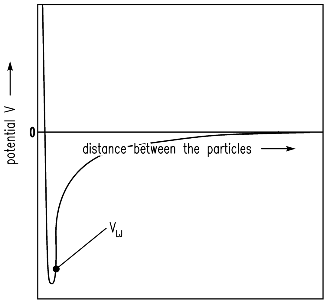
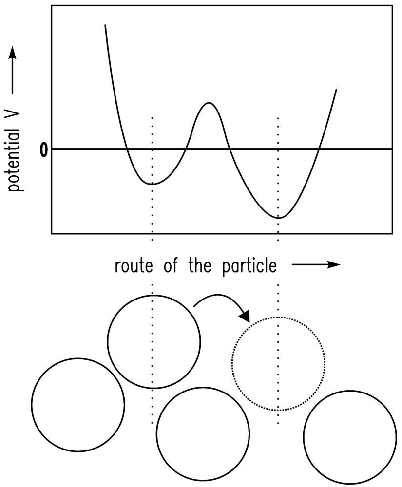
It is assumed that the driving forces for the consolidation are van der Waals forces [20]. The shrinkage is finally stopped by the remaining repulsive forces [24]. If there is a certain gel structure and van der Waals forces are applied to this structure, the structure will compact until further attraction is no longer possible because of the repulsive forces. The system is in equilibrium. Here, the sum of attractive (especially van der Waals) forces and repulsive forces is assumed to follow the Lennard-Jones (12-6) potential. In Figure 1, the Lennard-Jones (12-6) potential (V_LJ) [25] is shown qualitatively and the equilibrium condition (energy minimum) is obvious. In Figure 2, the motion of one particle is shown schematically. The Brownian motion, which is dependent on the temperature, causes the particle shown in Figure 2 to leave one minimum and reach another.

2.1. Model

2.1.1. Statistical Physics

The properties (in physics: position and momentum) of the systems of many particles (e.g., atoms, molecules, particles) are analyzed in statistical physics. Statistical ensembles are thus an important tool in statistical physics. An ensemble is an idealization consisting of a large number of copies of a system. These are considered all at once; each of them represents a possible state of the real system [26,27]. It is usual to investigate systems at constant pressure and constant temperature in an experimental situation. An isothermal isobaric ensemble (NPT ensemble) is an amount of systems of a given number of particles N, a given pressure p and a given temperature T [28].

The Ergodic hypothesis is the fundament of statistical physics. In the Ergodic hypothesis, it is assumed that the temporal average of a measured variable (e.g., of the pressure) is equal to the ensemble average:

$${\bar{\text{p}}}_{\text{t}}=〈\text{p}〉$$

(3)

2.1.2. MC vs. MD

Monte-Carlo (MC) simulations are especially appropriate for the calculation of statistical average values of a certain quantity. The Monte-Carlo method is—in the form it was developed by Metropolis et al. [6] and extended in several ways [29,30]—a procedure for estimating average values for ensembles of constant temperature, e.g., the isothermal isobaric ensemble. The quantities, pressure and temperature are defined in advance [31]. In molecular dynamics, Newton's equations of motion of N particles are numerically computed. An advantage of the MD method is that it delivers information about the temporal dependency and the extent of deviations of position and momentum, while MC is merely dealing with variables of position and does not provide any information about the temporal dependency of the deviations. It has been necessary to use the Monte-Carlo method in order to be able to fix the temperature and the pressure in a simulation, and abandons the possibility of gaining dynamical information in the same simulation [31]. Andersen [31] describes an MD method for performing simulations of a fluid at constant pressure without the loss of a dynamical description of the fluid. This method is a hybrid of MD and MC [32]. In Andersen's method, only changes in the volume of the MD simulation cell were possible, but not in its shape [33]. Parrinello and Rahman [33,34] have extended Andersen's method so that changes both of the volume and the shape of the MD cell become possible. Moreover, they have shown the usefulness of the application of their new method for changes in the structure of solids [32]. Nosé [32] proposes an MD method which can generate configurations belonging to the NPT ensemble by scaling time (with seconds) [35]. Hoover [35] developed a slightly different set of equations, free of time scaling. They both are referred to in the following.

2.1.3. MD Model

The consolidation of gel fragments is simulated by the MD tool, LAMMPS (Large-scale Atomic/Molecular Massively Parallel Simulator) [36]. The time integration in LAMMPS is performed on Nosé-Hoover-style equations of motion [32,35], which are designed to generate positions and velocities sampled from the isothermal isobaric (NPT) ensemble. This is achieved by adding dynamic variables which are coupled to the particle velocities (thermostating) and simulation domain dimensions (barostating). The external pressure of the barostat can be specified as either a scalar pressure (isobaric ensemble) or as components of a symmetric stress tensor (constant stress ensemble) [37]. The constant stress ensemble is used in the case of the simulation of the shrinkage of a gel fragment, and the isobaric ensemble is used for the simulation of the shrinkage of the particle network. The computations in the simulations here are carried out with dimensionless quantities. For the sake of being specific and clear about the equations used, they are repeated in the Appendix.

2.1.4. Structure of the Simulated Gel Fragment

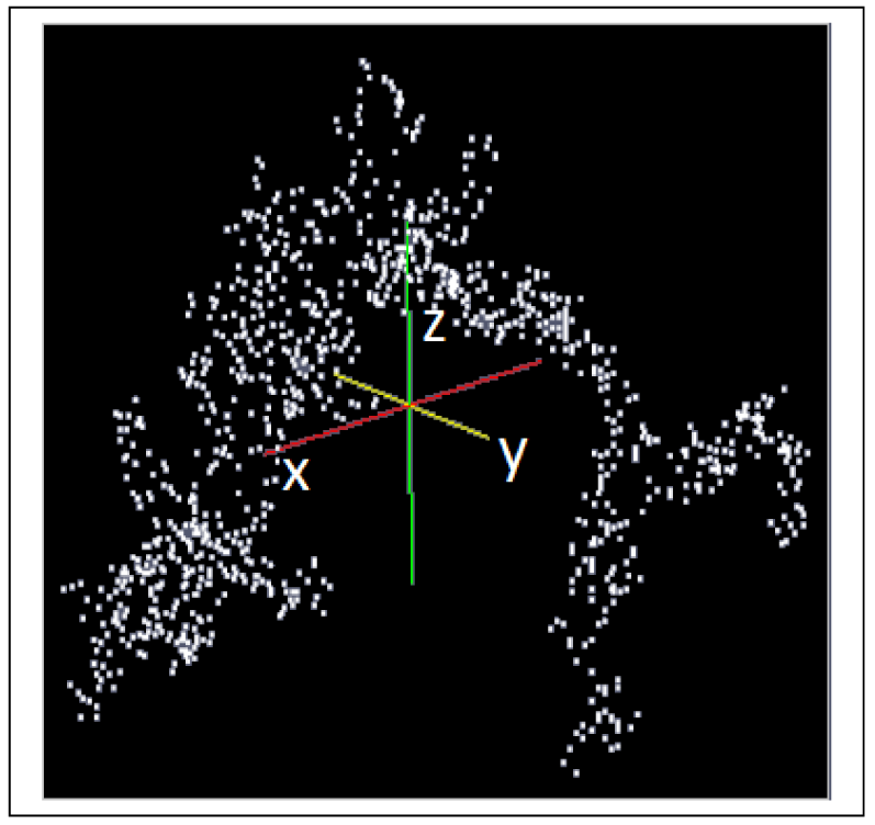
A fractal aggregate according to Schlomach and Kind (2007) [19] consisting of 1,000 primary particles (see Figure 3) is used for the simulation of the consolidation of a gel fragment. An algorithm based on a model developed by Sutherland (1967) [38] is used to generate this cluster consisting of primary particles. The collision probability for the cluster-cluster aggregation is obtained from the diffusion limited aggregation constant [39].

2.1.5. Interaction Energies

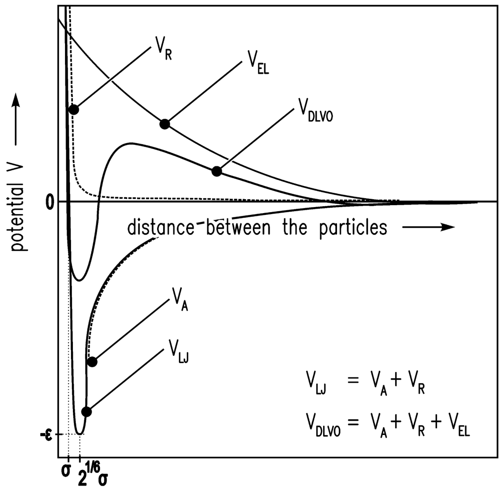
The solvent environment in the simulation is achieved by a high density lattice of solvent molecules. The Lennard-Jones (12-6) potential V [25] is used for the interaction energy between the solvent molecules of size σ.

$$\begin{array}{c}{V}_A=-\mathit{4}\epsilon {\left(\frac{\sigma }{r}\right)}^{\mathit{6}}\\ V_R=\mathit{4}\epsilon {\left(\frac{\sigma }{r}\right)}^{\mathit{12}}\\ V_{LJ}=V_A+V_R\end{array}$$

(4)

V_R describes Pauli/Born repulsion at short ranges due to overlapping electron orbitals, and V_A describes attraction at long ranges (mainly van der Waals attractive forces).

A colloidal particle has a size of 2a > σ. Evraers and Ejtehadi [41] describe each colloidal particle as an integrated collection of Lennard-Jones particles of size σ. Their formula for the colloid-colloid interaction energy between two particles gives with a₁ = a₂ = a (monodisperse):

$$\begin{array}{c}{V}_A=-\frac{A_{cc}}{6}\left[\frac{\mathit{2}{a}^{\mathit{2}}}{r^{\mathit{2}}-4a^2}+\frac{\mathit{2}{a}^{\mathit{2}}}{r^{\mathit{2}}}+ln\left(\frac{r^{\mathit{2}}-4a^{\mathit{2}}}{r^{\mathit{2}}}\right)\right]\hfill \\ V_R=\frac{A_{cc}}{37800}\frac{{\sigma }^6}{r}\left[\frac{r^{\mathit{2}}‐\mathit{14}ar+\mathit{54}{a}^{\mathit{2}}}{{(r‐\mathit{2}a)}^{\mathit{7}}}+\frac{r^{\mathit{2}}+\mathit{14}ar+\mathit{54}{a}^{\mathit{2}}}{{(r+\mathit{2}a)}^{\mathit{7}}}-\frac{\mathit{2}{r}^{\mathit{2}}‐6\mathit{0}{a}^{\mathit{2}}}{r^{\mathit{7}}}\right]\hfill \\ V_{LJ}=V_A+V_R\hfill \end{array}$$

(5)

where A_cc is the Hamaker constant and a is the radius of the colloidal particles.

The colloid-solvent interaction energy is given by

$$V_{LJ}=\frac{2a^3{\sigma }^3{A}_{cs}}{9{(a^2-r^2)}^3}\left[1-\frac{(\mathit{5}{a}^{\mathit{6}}+\mathit{45}{a}^{\mathit{4}}{r}^{\mathit{2}}+\mathit{63}{a}^{\mathit{2}}{r}^{\mathit{4}}+1\mathit{5}{r}^{\mathit{6}}){\sigma }^{\mathit{6}}}{\mathit{15}{(a‐r)}^{\mathit{6}}{(a+r)}^{\mathit{6}}}\right]$$

(6)

where A_cs is the Hamaker constant and a is the radius of the colloidal particles. This formula is derived from the colloid-colloid interaction energy formula (see [41]), letting one of the particle sizes be zero. Hence, pairwise interactions between large colloidal particles and small solvent particles are computed using these three formulas [37] in case of Lennard-Jones (LJ) interactions between particles. The additional electrostatic repulsive force (V_El) is added to the LJ potential for DLVO interactions(V_DLVO):

$$V_{\mathit{\text{DLVO}}}=V_{\mathit{\text{LJ}}}+V_{\mathit{\text{EL}}}$$

(7)

where

$$V_{\mathit{\text{EL}}}=\frac{A}{\kappa }\cdot exp\{-\kappa (r-2a)\}$$

(8)

with

$$A=2\pi a\epsilon {\epsilon }_0\kappa \cdot {\mathrm{\Psi }}^2$$

(9)

Here, ε is the relative permittivity of the fluid, ε₀ is the electric constant, κ is the inverse screening length, and ψ is the surface potential [37].

In Figure 4, the LJ potential (Equations (4–6)) and DLVO potential are shown.

2.2. Results and Discussion

2.2.1. Consolidation of a Single Cluster

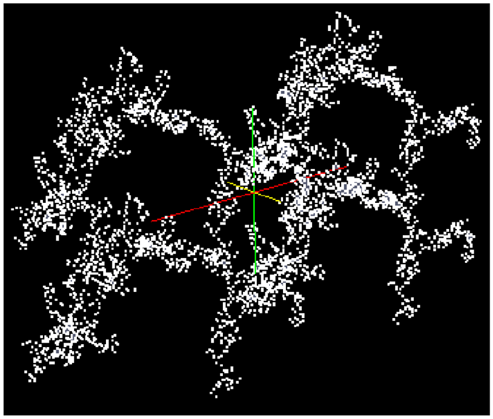
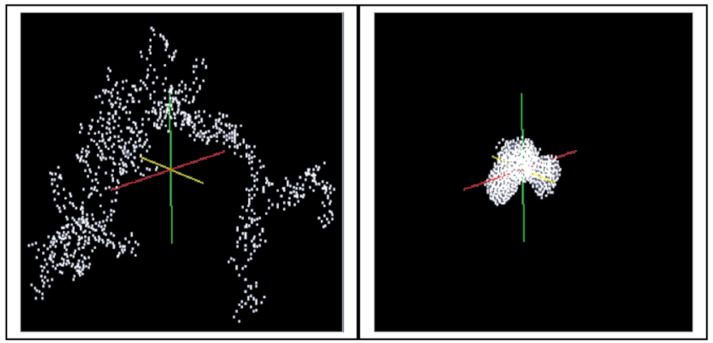
A cluster consisting of 1,000 particles in the environment of ∼400,000 solvent molecules is densified in LAMMPS as an isothermal isobaric (NPT) ensemble under the assumption of the interaction energies between the particles according to Equations (4–6) (LJ interactions). The isothermal isobaric ensemble was chosen in order to imitate the real situation where a gel cluster is confronted by a certain pressure in three dimensions in a stirred vessel. Thus, a certain temperature and a certain pressure can be allotted to the particle system. Figure 5 shows the computed model of a gel fragment before and after shrinkage.

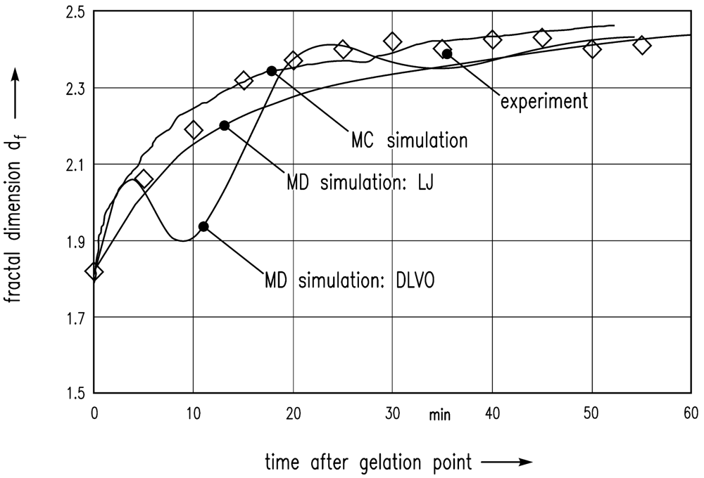
In the following, these simulation results are compared with the experiment of Schlomach and Kind [22]. Figure 6 shows data from a stirred vessel experiment [22], along with the MC simulation of Schlomach (2006) [40] and the simulated data (LJ) computed here. The fractal dimension is plotted as a function of the time after the gelation point. The formula for the computation of the fractal dimension d_f of the gel aggregates in the simulations is

$$r_{\mathit{\text{agg}}}=n^{\frac{1}{d_f}}\cdot r_p$$

(10)

where n is the number of primary particles in the aggregate, and r_agg and r_p are the radii of the aggregate and the primary particles, respectively. The agreement of the MD simulation with the experimental data is not as good as with the MC simulation. The theoretical MD curve matches the experimental data at the beginning and at the end of the simulation; there are deviations in between. The agreement shown of simulation data with the experimental data is admittedly only achieved by weighting the time step with a factor of 100 (1 min = 100 time steps). This indicates that the assumptions for the simulation are still incomplete. This concerns both the Lennard-Jones interaction energies between the particles as an approach for van der Waals and Pauli/Born interactions, and the use of an isothermal isobaric (NPT) ensemble. Apparently, the Nosé-Hoover thermostat as a deterministic method for the achievement of a constant temperature in the simulation (isothermal ensemble) is appropriate for the problem. Additionally, the equations used for the generation of an isobaric ensemble, and the assumption of van der Waals forces in interplay with the thermal motion as driving forces for the consolidation seem appropriate for the problem.

Furthermore, the electrostatic repulsive force according to Equation (8) was taken into account to achieve DLVO interactions between the particles. An additional MD simulation leads to the data shown in Figure 6. The results show that DLVO interactions are not appropriate for this problem.

2.2.2. Consolidation of a Particulate Network

In order to simulate the shrinkage of an expanded gel sample, the highly porous cluster (left side of Figure 4) is stringed together regularly in the x- and z-direction (25 × 40 clusters of 1,000 particles). Thus, a particulate network consisting of 10⁶ particles is generated. The kind of arrangement is shown in Figure 7 by means of 2 × 2 clusters.

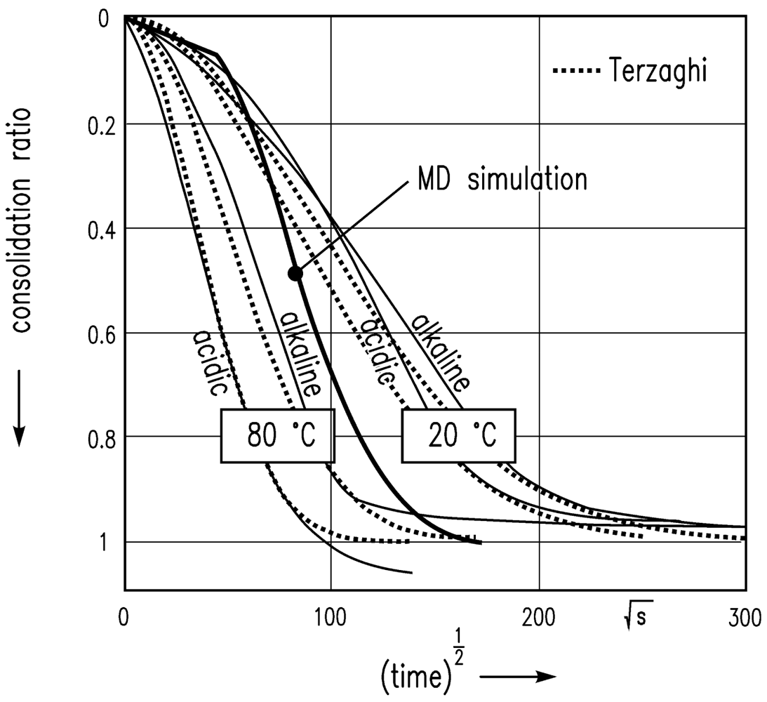
The simulation leads to the results shown in Figure 8 with the assumption of van der Waals attractive and Pauli/Born repulsive interaction energies between the particles, and consolidation in the z-direction at a constant temperature. A scalar pressure in the z direction is chosen in order to imitate the experimental situation of a gel sample in the oedometer test. The time step was weighted with factor 10 (1 min = 10 time steps) in order to bring the MD simulation results into reasonable agreement with experimental data.

The sharp bend of the consolidation ratio computed is because of the low resolution of the time step in the initial phase of this square-root-of-time plot.

2.3. Conclusions

The consolidation of gel fragments and of a particle network consisting of gel fragments have been investigated on the assumption of the interplay of van der Waals energies and thermal motion as driving forces for the shrinkage. Two molecular dynamics simulations have been performed with the tool LAMMPS: The fractal dimension of the MD simulation of the shrinkage of the gel fragment was compared to the results of a former MC simulation and also to experimental data. After time scale adjustment (factor 100) the simulation data could be aligned in agreement with the experimental data. Thus, the assumptions of the simulation have apparently been correct. Van der Waals forces in interplay with the thermal motion are considered to be driving forces for consolidation.

Furthermore, an MD simulation of the consolidation of a gel volume element was performed. The consolidation ratio of the consolidating particle network was compared to experimental data from oedometer tests. Good agreement of experiment and simulated data was also found here after time scale adjustment (factor 10). However, in order to describe the temporal course of the consolidation in more thoroughly, the fluid flow through the particle network needs to be taken into consideration. This has been neglected in the simulation so far. This coupling will, however, be investigated in the future.

References

- Evonik industries. Ultrasil®, Available online: http://ultrasil.evonik.de/PRODUCT/ULTRASIL/EN/ABOUT/Pages/default.aspx (accessed on 19 December 2011).
- Wacker Chemie, AG. Brochure HDK®—HDK® Pyrogenic Silica, Available online: http://www.wacker.com/cms/media/publications/downloads/6174_EN.pdf (accessed on 19 December 2011).
- Wacker Chemie, AG. Brochure Product Overview—HDK® Pyrogenic Silica, Available online: http://www.wacker.com/cms/media/publications/downloads/6180_EN.pdf (accessed on 19 December 2011).
- Becker, V.; Briesen, H. Tangential-force model for interactions between bonded colloidal particles. Phys. Rev. E 2008. [Google Scholar] [CrossRef]
- Brady, J.; Bossis, G. Stokesian dynamics. Ann. Rev. Fluid Mech. 1988, 20, 111–157. [Google Scholar]
- Metropolis, N.; Metropolis, A.W.; Rosenbluth, M.N.; Teller, A.H.; Teller, E. Equations of state calculations by fast computing machines. J. Chem. Phys. 1953, 21, 1087–1092. [Google Scholar]
- Doi, M.; Chen, D. Simulation of aggregating colloids in shear flow. J. Chem. Phys. 1989, 90, 5271–5279. [Google Scholar]
- Chen, D.; Doi, M. Simulation of aggregating colloids in shear flow. J. Chem. Phys. 1989, 91, 2656–2663. [Google Scholar]
- Doi, M.; Edwards, S.F. The Theory of Polymer Dynamics; Oxford University: Oxford, UK, 1986. [Google Scholar]
- Higashitani, K.; Iimura, K.; Sanda, H. Simulation of the deformation and breakup of large aggregates in flows of viscous fluids. Chem. Eng. Sci. 2001. [Google Scholar] [CrossRef]
- Verwey, E.J.; Overbeek, J.T.G. Theory of the Stability of Lyophobic Colloids; Elsevier Science: Amsterdam, The Netherlands, 1948. [Google Scholar]
- Hunter, J.R. Foundations of Colloid Science, 5th ed.; Oxford Science: Oxford, UK, 1995. [Google Scholar]
- Israelachvili, J.N. Intermolecular and Surface Forces, 2nd ed.; Academic Press: London, UK, 1991. [Google Scholar]
- Cundall, P.A. The Measurement Analysis of Accelerations in Rock Slopes. Ph.D. thesis, Imperial College, London, UK, 1971. [Google Scholar]
- Cundall, P.A.; Strack, O.D.L. A discrete numerical model for granular assemblies. Geotechnique 1979, 29, 47–65. [Google Scholar]
- Poeschel, P.; Schwager, T. Computational Granular Dynamics: Models and Algorithms, 2nd ed.; Springer Verlag: Berlin, Germany, 2005. [Google Scholar]
- Becker, V.; Briesen, H. Restructuring of colloidal aggregates in shear flows and limitations of the free-draining approximation. J. Colloid Interface Sci. 2009, 339, 362–372. [Google Scholar]
- Becker, V.; Briesen, H. A master curve for the onset of shear induced restructuring of fractal colloidal aggregates. J. Colloid Interface Sci. 2010, 346, 32–36. [Google Scholar]
- Schlomach, J.; Kind, M. Theoretical study of the reorganization of fractal aggregates by diffusion. Particul. Sci. Technol. 2007, 25, 519–533. [Google Scholar]
- Pierre, A.C.; Uhlmann, D.R. Better Ceramics through Chemistry III; Brinker, C.J., Clark, D.E., Ulrich, D.R., Eds.; Materials Research Society: Pittsburgh, PA, USA, 1988; pp. 207–212. [Google Scholar]
- Brinker, C.J.; Scherer, G.W. Aging of Gels: Aging Processes. In Sol-Gel Science: The Physics and Chemistry of Sol-Gel Processing; Academic Press Inc.: San Diego, CA, USA, 1990; p. 359. [Google Scholar]
- Schlomach, J.; Kind, M. Investigations on the semi-batch precipitation of silica. J. Colloid Interface Sci. 2004, 277, 316–326. [Google Scholar]
- Sahabi, H.; Kind, M. Consolidation of inorganic precipitated silica gel. Polymers 2011, 3, 1423–1432. [Google Scholar]
- Prakash, S.P.; Dhar, N.R. J. Indian Chem. Soc. 1930, 7, 417–434.
- Lennard-Jones, J.E. On the determination of molecular fields. Proc. R. Soc. Lond A 1924, 106, 463–477. [Google Scholar]
- Kittel, C.; Kroemer, H. Thermal Physics, 2nd ed.; W.H. Freeman and Company: San Francisco, CA, USA, 1980; p. 31. [Google Scholar]
- Landau, L.D.; Lifshitz, E.M. Statistical Physics; Pergamon Press: Oxford, UK, 1980; p. 9. [Google Scholar]
- Schwabl, F. Statistische Mechanik, 3rd ed.; Springer Verlag: Berlin, Germany, 2006. [Google Scholar]
- Valleau, J.P.; Whittington, S.G. A Guide to Monte Carlo for Statistical Mechanics: 1. Highways. In Statistical Mechanics, Part A: Equilibrium Techniques; Berne, B.J., Ed.; Plenum: New York, NY, USA, 1977; p. 137. [Google Scholar]
- Valleau, J.P.; Whittington, S.G. A Guide to Monte Carlo for Statistical Mechanics: 2. Byways. In Statistical Mechanics, Part A: Equilibrium Techniques; Berne, B.J., Ed.; Plenum: New York, NY, USA, 1977; p. 169. [Google Scholar]
- Andersen, H.C. Molecular dynamics simulations at constant pressure and/or temperature. J. Chem. Phys. 1980. [Google Scholar] [CrossRef]
- Nosé, S. A unified formulation of the constant temperature molecular-dynamics methods. J. Chem. Phys. 1984, 81, 511–519. [Google Scholar]
- Parrinello, M.; Rahman, A. Polymorphic transitions in single crystals: A new molecular dynamics method. J. Appl. Phys. 1981, 52, 7182–7190. [Google Scholar]
- Parrinello, M.; Rahman, A. Crystal structure and pair potentials: A molecular-dynamics study. Phys. Rev. Lett. 1980, 45, 1196–1199. [Google Scholar]
- Hoover, W.G. Canonical dynamics: Equilibrium phase-space distributions. Phys. Rev. A 1985, 31, 1695–1697. [Google Scholar]
- Plimpton, S.J. Fast parallel algorithms for short-range molecular dynamics. J. Comp. Phys. 1995, 117, 1–19. [Google Scholar]
- Sandia Corporation (© 2003). LAMMPS User's Manual: Large-Scale Atomic/Molecular Massively Parallel Simulator, Available online: http://lammps.sandia.gov (accessed on 19 December 2011).
- Sutherland, D.N. A theoretical model of floc structure. J. Colloid Interface Sci. 1967, 25, 373–380. [Google Scholar]
- Smoluchowski, M. Versuch einer mathematischen Theorie der Koagulationskinetik kolloidaler Lösungen. Z. Phys. Chem. 1917, 92, 129–168. [Google Scholar]
- Schlomach, J. Feststoffbildung bei technischen Fällprozessen. Ph.D. Thesis, Universität Fridericiana Karlsruhe, Karlsruhe, Germany, 2006. [Google Scholar]
- Everaers, E.; Ejtehadi, M.R. Interaction potentials for soft and hard ellipsoids. Phys. Rev. E 2003, 67, 041710. [Google Scholar]
- Shinoda, W.; Shiga, M.; Mikami, M. Rapid estimation of elastic constants by molecular dynamics simulation under constant stress. Phys. Rev. B 2004, 69, 134103. [Google Scholar]
- Martyna, G.J.; Tobias, D.J.; Klein, M.L. Constant pressure molecular dynamics algorithms. J. Chem. Phys. 1994. [Google Scholar] [CrossRef]
- Martyna, J.; Tuckerman, M.E.; Tobias, D.J.; Klein, M.L. Explicit reversible integration algorithms for extended systems. Mol. Phys. 1996, 87, 1117–1157. [Google Scholar]
- Brun, V. Carl Störmer in memoriam. Acta Math. 1958. [Google Scholar] [CrossRef]
- Verlet, L. Computer “experiments” on classical fluids. II. Equilibrium correlation functions. Phys. Rev. 1968, 165, 201–214. [Google Scholar]
- Tuckerman, M.E.; Berne, B.J.; Martyna, G.J. Reversible multiple time scale molecular dynamics. J. Chem. Phys. 1992. [Google Scholar] [CrossRef]
- Tuckerman, M.E.; Alejandre, J.; Lopez-Rendon, R.; Jochim, A.L.; Martyna, G.J. A Liouville-operator derived measure-preserving integrator for molecular dynamics simulations in the isothermal-isobaric ensemble. J. Phys. A Math. Gen. 2006. [Google Scholar] [CrossRef]