

Characterization and Kinetic Study of Agricultural Biomass Orange Peel Waste Combustion Using TGA Data
 ,
,  , , and
Abstract
1. Introduction
2. Materials and Methods
2.1. OP Material and TGA
2.2. Kinetics Equations
2.3. Thermodynamic Parameters of OP Combustion
3. Results and Discussion
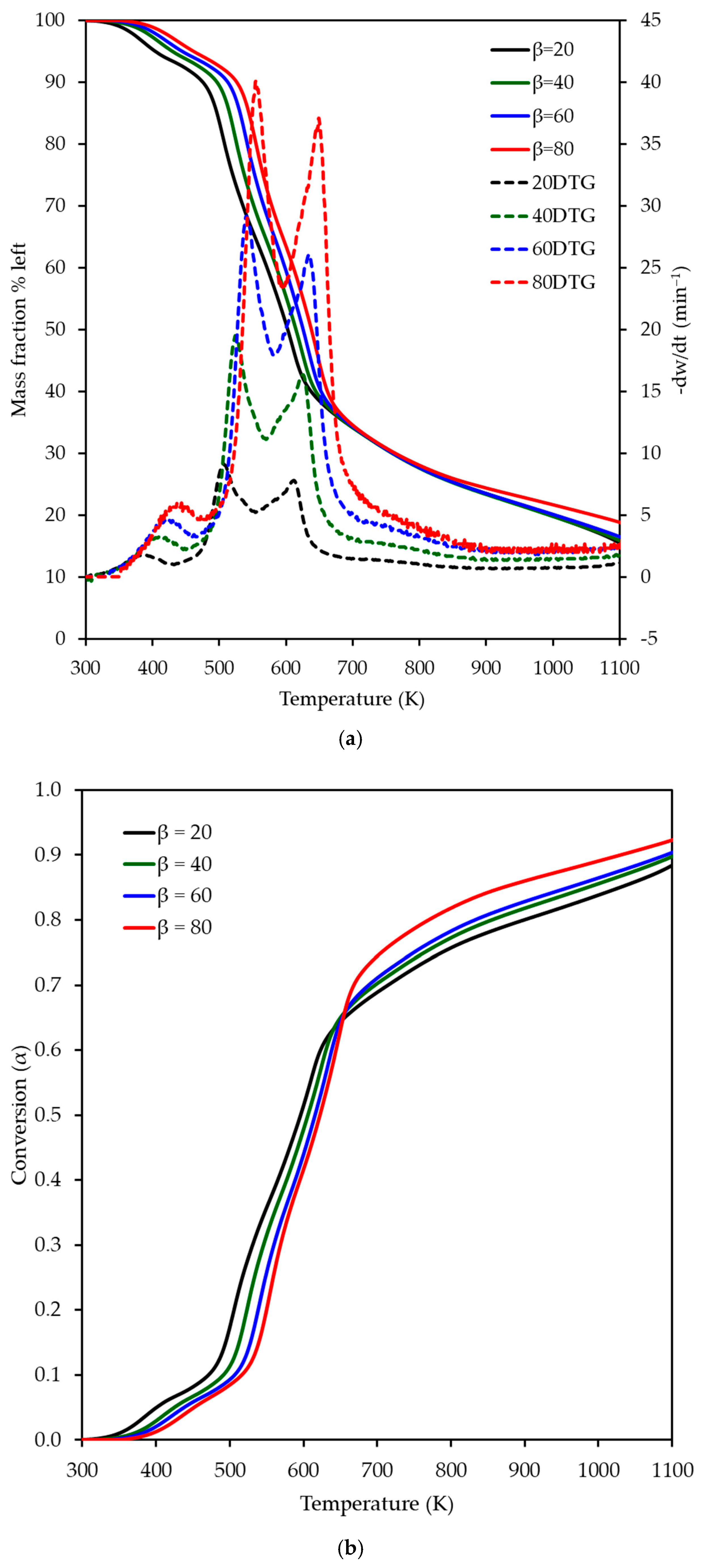
3.1. TG & DTG Analysis of OP Combustion
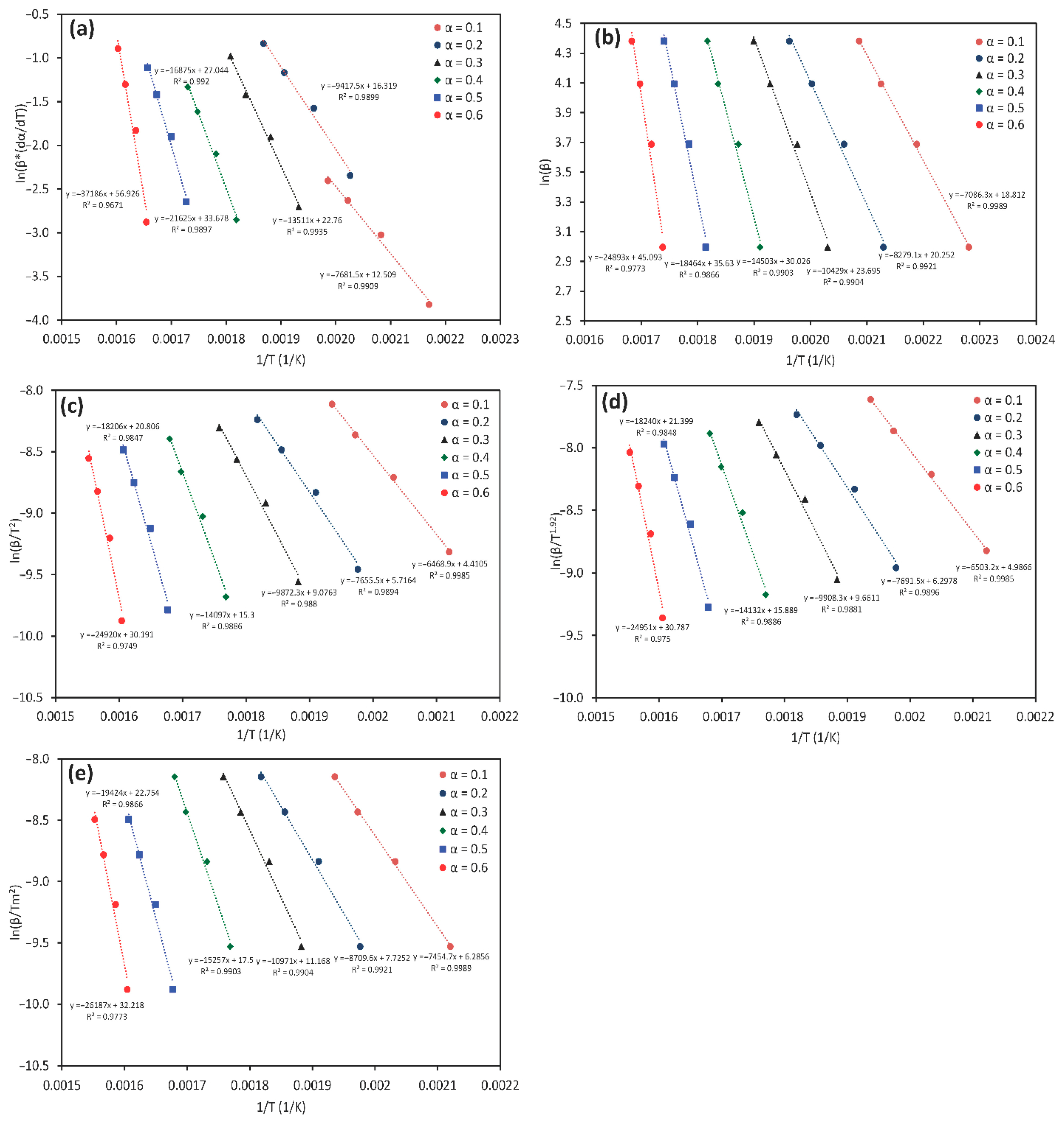
3.2. Model-Free Methods
3.3. CR Model-Fitting Method
3.4. Thermodynamic Parameters

| α | FR | FWO | ||||||||
|---|---|---|---|---|---|---|---|---|---|---|
| R2 | A0 (min−1) | ΔH (kJ mol−1) | ΔG (kJ mol−1) | ΔS (kJ mol−1) | R2 | A0 (min−1) | ΔH (kJ mol−1) | ΔG (kJ/mol−1) | ΔS (kJ/mol−1) | |
| 0.1 | 0.9909 | 6.68 × 10³ | 60.63 | 134.57 | −0.18255 | 0.9989 | 5.13 × 10⁹ | 55.63 | 83.94 | −0.06989 |
| 0.2 | 0.9899 | 6.78 × 10⁵ | 73.64 | 150.44 | −0.1463 | 0.9921 | 7.99 × 10¹⁰ | 64.64 | 90.48 | −0.04922 |
| 0.3 | 0.9935 | 7.27 × 10⁸ | 107.64 | 153.99 | −0.08829 | 0.9904 | 4.85 × 10¹² | 82.64 | 90.56 | −0.01509 |
| 0.4 | 0.9920 | 8.16 × 10¹⁰ | 135.64 | 161.38 | −0.04904 | 0.9903 | 3.82 × 10¹⁵ | 116.64 | 95.45 | 0.040362 |
| 0.5 | 0.9897 | 9.23 × 10¹³ | 174.80 | 169.82 | 0.007967 | 0.9866 | 1.41 × 10¹⁸ | 148.80 | 93.75 | 0.088086 |
| 0.6 | 0.9671 | 1.71 × 1024 | 303.80 | 175.98 | 0.204512 | 0.9773 | 2.20 × 10²² | 201.80 | 96.58 | 0.168352 |
| α | KAS | STK | ||||||||
| R2 | A0 (min−1) | ΔH (kJ mol−1) | ΔG (kJ mol−1) | ΔS (kJ mol−1) | R2 | A0 (min−1) | ΔH (kJ mol−1) | ΔG (kJ mol−1) | ΔS kJ mol−1 | |
| 0.1 | 0.9985 | 6.37 × 10² | 50.63 | 132.48 | −0.2021 | 0.9985 | 2.69 × 101 | 50.63 | 143.14 | −0.22842 |
| 0.2 | 0.9894 | 1.20 × 10⁴ | 59.64 | 154.05 | −0.17983 | 0.9896 | 3.63 × 10² | 59.64 | 169.32 | −0.20893 |
| 0.3 | 0.988 | 1.08 × 10⁶ | 77.64 | 152.39 | −0.1424 | 0.9881 | 2.00 × 10⁴ | 77.64 | 169.82 | −0.17559 |
| 0.4 | 0.9886 | 1.52 × 10⁹ | 112.64 | 155.76 | −0.08214 | 0.9886 | 1.39 × 10⁷ | 112.64 | 176.27 | −0.12122 |
| 0.5 | 0.9847 | 8.40 × 10¹¹ | 145.80 | 165.25 | −0.03111 | 0.9848 | 4.58 × 10⁹ | 146.80 | 193.33 | −0.07444 |
| 0.6 | 0.9749 | 2.23 × 10¹⁶ | 201.80 | 168.31 | 0.05359 | 0.975 | 6.53 × 10¹³ | 201.80 | 198.62 | 0.00509 |
| α | K | |||||||||
| R2 | A0 (min−1) | ΔH (kJ mol−1) | ΔG (kJ mol−1) | ΔS (kJ mol−1) | ||||||
| 0.1 | 0.9989 | 4.00 × 10⁶ | 58.63 | 111.03 | −0.12938 | |||||
| 0.2 | 0.9921 | 1.96 × 10⁷ | 67.64 | 129.76 | −0.11832 | |||||
| 0.3 | 0.9904 | 7.75 × 10⁸ | 86.64 | 132.71 | −0.08775 | |||||
| 0.4 | 0.9903 | 6.08 × 10¹¹ | 122.64 | 139.61 | −0.03234 | |||||
| 0.5 | 0.9866 | 1.48 × 10¹⁴ | 155.80 | 148.39 | 0.011866 | |||||
| 0.6 | 0.9773 | 2.57 × 10¹⁸ | 212.8038 | 154.6353 | 0.09307 | |||||
4. Conclusions
Author Contributions
Funding
Institutional Review Board Statement
Data Availability Statement
Conflicts of Interest
References
- Saidur, R.; Abdelaziz, E.A.; Demirbas, A.; Hossain, M.S.; Mekhilef, S. A review on biomass as a fuel for boilers. Renew. Sustain. Energy Rev. 2011, 15, 2262–2289. [Google Scholar] [CrossRef]
- Chilla, V.; Suranani, S. Thermogravimetric and kinetic analysis of orange peel using isoconversional methods. Mater. Today Proc. 2023, 72, 104–109. [Google Scholar] [CrossRef]
- Bridgeman, T.G.; Jones, J.M.; Shield, I.; Williams, P.T. Torrefaction of reed canary grass, wheat straw and willow to enhance solid fuel qualities and combustion properties. Fuel 2008, 87, 844–856. [Google Scholar] [CrossRef]
- Pimchuai, A.; Dutta, A.; Basu, P. Torrefaction of agriculture residue to enhance combustible properties. Energy Fuels 2010, 24, 4638–4645. [Google Scholar] [CrossRef]
- Lopez-Velazquez, M.A.; Santes, V.; Balmaseda, V.; Torres-Garcia, E. Pyrolysis of orange waste: A thermo-kinetic study. J. Anal. Appl. Pyrolysis 2013, 99, 170–177. [Google Scholar] [CrossRef]
- Anca-Couce, A.; Berger, A.; Zobel, N. How to determine consistent biomass pyrolysis kinetics in a parallel reaction scheme. Fuel 2014, 123, 230–240. [Google Scholar] [CrossRef]
- Santos, C.M.; Dweck, J.; RenataViotto, R.S.; Rosa, A.H.; Morais, L.C.D. Application of orange peel waste in the production of solid biofuels and biosorbents. Bioresour. Technol. 2015, 196, 469–479. [Google Scholar] [CrossRef] [PubMed]
- Indulekha, J.; Siddarth, M.G.; Kalaichelvi, P.; Arunagiri, A. Characterization of citrus peels for bioethanol production. In Materials, Energy and Environment Engineering; Springer: Singapore, 2017; pp. 3–12. [Google Scholar] [CrossRef]
- Zhu, Y.; Xu, G.; Song, W.; Zhao, Y.; Miao, Z.; Yao, R.; Gao, J. Catalytic microwave pyrolysis of orange peel: Effects of acid and base catalysts mixture on products distribution. J. Energy Inst. 2021, 98, 172–178. [Google Scholar] [CrossRef]
- Açıkalın, K. Evaluation of orange and potato peels as an energy source: A comprehensive study on their pyrolysis characteristics and kinetics. Biomass Convers. Biorefinery 2022, 12, 501–514. [Google Scholar] [CrossRef]
- Hosseinzaei, B.; Hadianfard, M.J.; Aghabarari, B.; García-Rollán, M.; Ruiz-Rosas, R.; Rosas, J.M.; Rodríguez-Mirasol, J.; Cordero, T. Pyrolysis of pistachio shell, orange peel and saffron petals for bioenergy production. Bioresour. Technol. Rep. 2022, 19, 101209. [Google Scholar] [CrossRef]
- Selvarajoo, A.; Wong, Y.L.; Khoo, K.S.; Hen, W.H.; Show, P.S. Biochar production via pyrolysis of citrus peel fruit waste as a potential usage as solid biofuel. Chemosphere 2022, 294, 133671. [Google Scholar] [CrossRef] [PubMed]
- Tariq, R.; Zaifullizan, Y.M.; Salema, A.A.; Abdulatif, A.; Ken, L.S. Co-pyrolysis and co-combustion of orange peel and biomass blends: Kinetics, thermodynamic, and ANN application. Renew. Energy 2022, 198, 399–414. [Google Scholar] [CrossRef]
- Kim, J.H.; Lee, T.; Tsang, Y.F.; Moon, D.H.; Lee, J.; Kwon, E.E. Functional use of carbon dioxide for the sustainable valorization of orange peel in the pyrolysis process. Sci. Total Environ. 2024, 941, 173701. [Google Scholar] [CrossRef]
- Kwon, D.; Oh, J.I.; Lam, S.S.; Moon, D.H.; Kwon, E.E. Orange peel valorization by pyrolysis under the carbon dioxide environment. Bioresour. Technol. 2019, 285, 121356. [Google Scholar] [CrossRef] [PubMed]
- Zapata, B.; Balmaseda, J.; Fregoso-Israel, E.; Torres-García, E. Thermo-kinetics study of orange peel in air. J. Therm. Anal. Calorim. 2009, 98, 309–315. [Google Scholar] [CrossRef]
- Yaradoddi, J.S.; Banapurmath, N.R.; Ganachari, S.V.; Soudagar, M.E.M.; Sajjan, A.M.; Kamat, S.; Mujtaba, M.A.; Shettar, A.S.; Anqi, A.E.; Safaei, M.R.; et al. Bio-based material from fruit waste of orange peel for industrial applications. J. Mater. Res. Technol. 2022, 17, 3186–3197. [Google Scholar] [CrossRef]
- Kariim, I.; Park, J.Y.; Kazmi, W.W.; Swai, H.; Lee, I.G.; Kivevele, T. Solvothermal liquefaction of orange peels into biocrude: An experimental investigation of biocrude yield and energy compositional dependency on process variables. Bioresour. Technol. 2024, 391, 129928. [Google Scholar] [CrossRef] [PubMed]
- Divyabharathi, R.; Subramanian, P. Biocrude production from orange (Citrusreticulata) peel by hydrothermal liquefaction and process optimization. Biomass Convers. Biorefinery 2021, 12, 183–194. [Google Scholar] [CrossRef]
- López, J.Á.S.; Li, Q.; Thompson, I.P. Biorefinery of waste orange peel. Crit. Rev. Biotechnol. 2010, 30, 63–69. [Google Scholar] [CrossRef]
- Zaid Abdulhamid Alhulaybi, Z.A.; Dubdub, I. Kinetics Study of PVA Polymer by Model-Free and Model-Fitting Methods Using TGA. Polymers 2024, 16, 629. [Google Scholar] [CrossRef]
- Dhyani, V.; Kumar, J.; Bhaskar, T. Thermal Decomposition Kinetics of Sorghum Straw via Thermogravimetric Analysis. Bioresour. Technol. 2017, 245, 1122–1129. [Google Scholar] [CrossRef]
- Ou, C.; Chen, S.; Liu, Y.; Shao, J.; Li, S.; Fu, T.; Fan, W.; Zheng, H.; Lu, Q.; Bi, X. Study on the thermal degradation kinetics and pyrolysis characteristics of Chitosan-Zn complex. J. Anal. Appl. Pyrolysis 2016, 122, 268–276. [Google Scholar] [CrossRef]
- Coats, A.W.; Redfern, J.P. Kinetic Parameters from Thermogravimetric Data. Nature 1965, 207, 209. [Google Scholar] [CrossRef]
- Galwey, A.K. Eradicating erroneous Arrhenius arithmetic. Thermochim. Acta 2003, 399, 1–29. [Google Scholar] [CrossRef]
- Yao, Z.; Romano, P.; Fan, W.; Gautam, S.; Tippayawong, N.; Jaroenkhasemmeesuk, C.; Liu, J.; Wang, X.; Qi, W. Probing pyrolysis conversion of separator from spent lithium-ion batteries: Thermal behavior, kinetics, evolved gas analysis and Aspen Plus modeling. Case Stud. Therm. Eng. 2024, 63, 105342. [Google Scholar] [CrossRef]
- Tong, W.; Cai, Z.; Liu, Q.; Ren, S.; Kong, M. Effect of pyrolysis temperature on bamboo char combustion: Reactivity, kinetics and thermodynamics. Energy 2020, 211, 118736. [Google Scholar] [CrossRef]
- Huang, L.; Liu, J.; He, Y.; Sun, S.; Chen, J.; Sun, J.; Chang, K.; Kuo, J.; Ning, X. Thermodynamics and kinetics parameters of co-combustion between sewage sludge and water hyacinth in CO2/O2 atmosphere as biomass to solid biofuel. Bioresour. Technol. 2016, 218, 631–642. [Google Scholar] [CrossRef]
- Liu, H.; Wang, C.; Zhang, J.; Zhao, W.; Fan, M. Pyrolysis Kinetics and Thermodynamics of Typical Plastic Waste. Energy Fuels 2022, 34, 2385–2390. [Google Scholar] [CrossRef]
- Kalidasan, B.; Pandey, A.K.; Aljafari, B.; Chinnasamy, S.; Kareri, T.; Rahman, S. Thermo-kinetic behaviour of green synthesized nanomaterial enhanced organic phase change material: Model fitting approach. J. Environ. Manag. 2023, 348, 119439. [Google Scholar] [CrossRef]
- Ali, L.; Kuttiyathil, M.S.; Al-Harahsheh, M.; Altarawneh, M. Kinetic parameters underlying hematite-assisted decomposition of tribromophenol. Arab. J. Chem. 2023, 16, 3. [Google Scholar] [CrossRef]

| Reference | Heating Rate K min−1 | 1st Reaction | 2nd Reaction | 3rd Reaction | 4th Reaction | ||||||||
|---|---|---|---|---|---|---|---|---|---|---|---|---|---|
| T Range, T Peak (K) | Weight Loss % | Process | T Range, T Peak (K) | Weight Loss % | Process | T Range, T Peak (K) | Weight Loss % | Process | T Range, T Peak (K) | Weight Loss % | Process | ||
| Santos (2015) et al. [7] | 10 | 298–383, 323 | 10 | dehydration | 383–498, 473 | 20 | Hemicellulose degradation | 498–648, 573 | 40 | Cellulose degradation | 648–773, 723 | 20 | Lignin degradation |
| 15 | 298–398, 343 | 10 | Cellulose degradation | 398–513, 486 | 20 | Hemicellulose degradation | 513–663, 593 | 40 | Cellulose degradation | 663–778, 733 | 20 | Lignin degradation | |
| 20 | 298–403, 348 | 10 | Cellulose degradation | 403–523, 498 | 20 | Hemicellulose degradation | 523–673, 603 | 40 | Cellulose degradation | 673–793, 748 | 20 | Lignin degradation | |
| Tariq et al. (2022) [13] | 5 | 298–383, 323 | 10 | Cellulose degradation | 383–513, 465 | 30 | Hemicellulose degradation | 513–623, 553 | 30 | Cellulose degradation | 623–733, 688 | 20 | Lignin degradation |
| 10 | 298–403, 333 | 10 | Cellulose degradation | 403–523, 477 | 30 | Hemicellulose degradation | 523–633, 570 | 30 | Cellulose degradation | 633–773, 713 | 20 | Lignin degradation | |
| 15 | 298–410, 343 | 10 | Cellulose degradation | 410–543, 482 | 30 | Hemicellulose degradation | 543–643, 573 | 30 | Cellulose degradation | 643–783, 705 | 20 | Lignin degradation | |
| 20 | 298–423, 353 | 10 | Cellulose degradation | 423–553, 491 | Hemicellulose degradation | 553–653, 585 | 30 | Cellulose degradation | 653–793, 723 | 20 | Lignin degradation | ||
| Yaradoddi (et al.) (2022) [17] | 10 | 315–446, 364 | 12.5 | Cellulose degradation | 447–501, 473 | 59.4 | Hemicellulose & Cellulose degradation | 501–607, 553 | 10.6 | NA * | 573–673, 623 | 4.5 | Lignin degradation |
| Kim et al. (2024) [14] | 10 | 298–373, 343 | 10 | NA * | 373–543, 498 | 20 | NA * | 543–673, 580 | 40 | NA * | 673, | 25 | NA * |
| Proximate Analysis (wt.%) | Ultimate Analysis (wt.%) | ||
|---|---|---|---|
| Moisture content | 5.03 | C | 36.05 |
| Volatile matter | 69.5 | H | 3.601 |
| Ash | 5.5 | N | 13.27 |
| Fixed carbon a | 19.9 | S | 3.901 |
| O b | 43.176 | ||
| Model-Free Methods | |||
|---|---|---|---|
| Method | Formula | Plot | |
| FR | (4) | ||
| FWO | (5) | ||
| KAS | (6) | ||
| STK | (7) | ||
| K | (8) | ||
| VY | (9) | minimizing the function | |
| Model-fitting methods | |||
| Method | Formula | Plot | |
| CR | (10) | ||
| Reaction Mechanism | Code | f(α) | g(α) |
|---|---|---|---|
| Reaction order models–First order | F1 | 1 − α | |
| Reaction order models–Second order | F2 | ||
| Reaction order models–Third order | F3 | ||
| Diffusion model–One-dimensional | D1 | ||
| Diffusion model–Two-dimensional | D2 | ||
| Diffusion model–Three-dimensional | D3 | ||
| Diffusion model–Four-dimensional | D4 | 1.5 × [(1 − α)1/3 – 1] | 1 − (2/3) × α − (1 − α)2/3 |
| Nucleation models–Two-dimensional | A2 | ||
| Nucleation models–Three-dimensional | A3 | ||
| Nucleation models–Four-dimensional | A4 | ||
| Geometrical contraction models–One-dimensional; | R1 | 1 | |
| Geometrical contraction models—Sphere | R2 | ||
| Geometrical contraction models—Cylinder | R3 | ||
| Nucleation models–2-Power law | P2 | ||
| Nucleation models–3-Power law | P3 | ||
| Nucleation models–4-Power law | P4 |
| Heating Rate (K min−1) | 1st Reaction | 2nd Reaction | 3rd Reaction | ||||||
|---|---|---|---|---|---|---|---|---|---|
| T Range, T Peak (K) | Weight Loss % | Process | T Range, T Peak (K) | Weight Loss % | Process | T Range, T Peak (K) | Weight Loss % | Process | |
| 20 | 362–436, 380 | 8 | Dehydration | 436–554, 514 | 25 | Hemicellulose & Cellulose degradation | 554–666, 616 | 29 | Cellulose & Lignin degradation |
| 40 | 364–454, 416 | 8 | Dehydration | 454–572, 526 | 25 | Hemicellulose & Cellulose degradation | 572–692, 628 | 29 | Cellulose & Lignin degradation |
| 60 | 378–464, 420 | 8 | Dehydration | 464–586, 541 | 25 | Hemicellulose & Cellulose degradation | 586–698, 638 | 29 | Cellulose & Lignin degradation |
| 80 | 380–480, 438 | 8 | Dehydration | 480–595, 553 | 25 | Hemicellulose & Cellulose degradation | 595–732, 650 | 29 | Cellulose & Lignin degradation |
| Conversion | FR | FWO | KAS | STK | K | VY | Average | |||||||
|---|---|---|---|---|---|---|---|---|---|---|---|---|---|---|
| E (kJ mol−1) | R2 | E (kJ mol−1) | R2 | E (kJ mol−1) | R2 | E (kJ mol−1) | R2 | E (kJ mol−1) | R2 | E (kJ mol−1) | R2 | E (kJ mol−1) | R2 | |
| 0.1 | 64 | 0.9909 | 59 | 0.9989 | 54 | 0.9985 | 54 | 0.9985 | 62 | 0.9989 | 34 | NA * | 55 | 0.9005 |
| 0.2 | 78 | 0.9899 | 69 | 0.9921 | 64 | 0.9894 | 64 | 0.9896 | 72 | 0.9921 | 55 | NA * | 67 | 0.9408 |
| 0.3 | 112 | 0.9935 | 87 | 0.9904 | 82 | 0.988 | 82 | 0.9881 | 91 | 0.9904 | 97 | NA * | 92 | 0.9659 |
| 0.4 | 140 | 0.992 | 121 | 0.9903 | 117 | 0.9886 | 117 | 0.9886 | 127 | 0.9903 | 130 | NA * | 125 | 0.9879 |
| 0.5 | 180 | 0.9897 | 154 | 0.9866 | 151 | 0.9847 | 152 | 0.9848 | 161 | 0.9866 | 108 | NA * | 151 | 0.9900 |
| 0.6 | 309 | 0.9671 | 207 | 0.9773 | 207 | 0.9749 | 207 | 0.975 | 218 | 0.9773 | 113 | NA * | 210 | 0.9971 |
| Average | 147 | 0.9872 | 116 | 0.9893 | 113 | 0.9874 | 113 | 0.9874 | 122 | 0.9893 | 90 | NA * | 117 | 0.9712 |
| Reference | Model-Free Method | 1st Reaction | 2nd Reaction | 3rd Reaction | ||||||
|---|---|---|---|---|---|---|---|---|---|---|
| Ea (kJ mol−1) | R2 | Ea (kJ mol−1) | R2 | Ea (kJ mol−1) | R2 | |||||
| Santos et al. (2015) [7] | K | 113 | 0.9976 | 121 | 0.9579 | 179 | 0.9709 | |||
| Tariq et al. (2022) [13] | Ea (kJ mol−1) | |||||||||
| α = 0.1 | 0.2 | 0.3 | 0.4 | 0.5 | 0.6 | 0.7 | 0.8 | 0.9 | ||
| FWO | 70 | 105 | 130 | 150 | 130 | 100 | 80 | 140 | 125 | |
| KAS | 80 | 105 | 120 | 125 | 110 | 100 | 75 | 120 | 110 | |
| STK | 75 | 105 | 120 | 125 | 120 | 100 | 75 | 125 | 125 | |
| Reaction mechanism 1-step reaction | Code | 20 | 40 | 60 | ||||||
|---|---|---|---|---|---|---|---|---|---|---|
| Ea (kJ mol−1) | Ln(A0) | R2 | Ea (kJ mol−1) | Ln(A0) | R2 | Ea (kJ mol−1) | Ln(A0) | R2 | ||
| Reaction order models–First order | F1 | 29 | 17.34 | 0.996 | 33 | 17.52 | 0.9972 | 32 | 18.71 | 0.9977 |
| Reaction order models–Second order | F2 | 30 | 17.18 | 0.9962 | 34 | 17.37 | 0.9973 | 32 | 18.53 | 0.9978 |
| Reaction order models–Third order | F3 | 30 | 16.98 | 0.9965 | 34 | 17.19 | 0.9975 | 33 | 18.38 | 0.9979 |
| Diffusion models–One-dimensional | D1 | 63 | 13.06 | 0.9967 | 72 | 15.3 | 0.9976 | 69 | 14.07 | 0.9981 |
| Diffusion models–Two-dimensional | D2 | 64 | 12.51 | 0.9967 | 72 | 14.72 | 0.9976 | 69 | 13.5 | 0.9981 |
| Diffusion models–Three-dimensional | D3 | 64 | 12.76 | 0.9968 | 73 | 13.34 | 0.9977 | 70 | 14.14 | 0.9981 |
| Diffusion models–Four-dimensional | D4 | 64 | 12.84 | 0.9967 | 73 | 13.27 | 0.9976 | 6 | 22.16 | 0.992 |
| Nucleation models–Two-dimensional | A2 | 11 | 20.22 | 0.9931 | 13 | 20.8 | 0.9953 | 12 | 21.57 | 0.996 |
| Nucleation models–Three-dimensional | A3 | 5 | 20.71 | 0.9861 | 7 | 21.59 | 0.9912 | 6 | 22.16 | 0.992 |
| Nucleation models–Four-dimensional | A4 | 2 | 20.44 | 0.9618 | 3 | 21.44 | 0.9794 | 3 | 22.11 | 0.978 |
| Geometrical contraction models–One-dimensional phase boundary | R1 | 28 | 17.49 | 0.9958 | 33 | 17.69 | 0.997 | 31 | 18.86 | 0.9976 |
| Geometrical contraction models–Contracting sphere | R2 | 29 | 18.13 | 0.9959 | 33 | 18.3 | 0.9971 | 31 | 19.47 | 0.9976 |
| Geometrical contraction models–Contracting cylinder | R3 | 29 | 18.5 | 0.9959 | 33 | 18.67 | 0.9971 | 31 | 19.84 | 0.9976 |
| Nucleation models–Power law | P2 | 11 | 20.31 | 0.9926 | 13 | 20.89 | 0.9949 | 12 | 21.67 | 0.9957 |
| Nucleation models–Power law | P3 | 5 | 20.78 | 0.9848 | 6 | 21.49 | 0.9904 | 6 | 22.22 | 0.9913 |
| Nucleation models–Power law | P4 | 2 | 20.49 | 0.9565 | 3 | 21.49 | 0.9771 | 3 | 22.15 | 0.9751 |
| Reaction mechanism 1-step reaction | Code | 80 | ||||||||
| Ea (kJ mol−1) | Ln(A0) | R2 | ||||||||
| Reaction order models–First order | F1 | 34 | 18.61 | 0.9979 | ||||||
| Reaction order models–Second order | F2 | 35 | 18.45 | 0.998 | ||||||
| Reaction order models–Third order | F3 | 36 | 18.3 | 0.9981 | ||||||
| Diffusion models–One-dimensional | D1 | 71 | 15.36 | 0.9982 | ||||||
| Diffusion models–Two-dimensional | D2 | 75 | 14.84 | 0.9982 | ||||||
| Diffusion models–Three-dimensional | D3 | 76 | 13.54 | 0.9983 | ||||||
| Diffusion models–Four-dimensional | D4 | 75 | 13.6 | 0.9982 | ||||||
| Nucleation models–Two-dimensional | A2 | 14 | 21.82 | 0.9964 | ||||||
| Nucleation models–Three-dimensional | A3 | 7 | 22.49 | 0.9932 | ||||||
| Nucleation models–Four-dimensional | A4 | 3 | 23.32 | 0.9832 | ||||||
| Geometrical contraction models–One-dimensional phase boundary | R1 | 34 | 18.79 | 0.9977 | ||||||
| Geometrical contraction models–Contracting sphere | R2 | 34 | 19.39 | 0.9978 | ||||||
| Geometrical contraction models–Contracting cylinder | R3 | 34 | 19.77 | 0.9978 | ||||||
| Nucleation models–Power law | P2 | 13 | 21.83 | 0.9962 | ||||||
| Nucleation models–Power law | P3 | 7 | 22.46 | 0.9926 | ||||||
| Nucleation models–Power law | P4 | 3 | 22.37 | 0.9812 | ||||||
| Reaction mechanism 2-step reaction | Code | 20 | 40 | 60 | ||||||
| Ea (kJ mol−1) | Ln(A0) | R2 | Ea (kJ mol−1) | Ln(A0) | R2 | Ea (kJ mol−1) | Ln(A0) | R2 | ||
| Reaction order models–First order | F1 | 43 | 15.35 | 0.9928 | 55 | 13.9 | 0.9972 | 58 | 14.13 | 0.9971 |
| Reaction order models–Second order | F2 | 49 | 13.83 | 0.9945 | 61 | 12.66 | 0.9964 | 66 | 13.82 | 0.998 |
| Reaction order models–Third order | F3 | 56 | 12.19 | 0.9957 | 67 | 14.32 | 0.9956 | 75 | 16.03 | 0.9987 |
| Diffusion models–One-dimensional | D1 | 82 | 16.01 | 0.9925 | 107 | 22.04 | 0.9981 | 109 | 22.2 | 0.9966 |
| Diffusion models–Two-dimensional | D2 | 86 | 16.34 | 0.9931 | 111 | 22.28 | 0.9979 | 114 | 22.7 | 0.9969 |
| Diffusion models–Three-dimensional | D3 | 90 | 15.9 | 0.9936 | 115 | 21.75 | 0.9977 | 119 | 22.45 | 0.9973 |
| Diffusion models–Four-dimensional | D4 | 87 | 15.19 | 0.9932 | 112 | 21.1 | 0.9979 | 116 | 21.62 | 0.997 |
| Nucleation models–Two-dimensional | A2 | 17 | 19.75 | 0.9885 | 23 | 19.57 | 0.9961 | 24 | 19.95 | 0.9959 |
| Nucleation models–Three-dimensional | A3 | 9 | 20.9 | 0.9794 | 13 | 21.17 | 0.9944 | 13 | 21.57 | 0.9936 |
| Nucleation models–Four-dimensional | A4 | 4 | 20.97 | 0.9543 | 7 | 21.65 | 0.9909 | 8 | 22.3 | 0.9892 |
| Geometrical contraction models–One-dimensional phase boundary | R1 | 37 | 16.72 | 0.9906 | 49 | 15.17 | 0.9978 | 50 | 15.78 | 0.9959 |
| Geometrical contraction models–Contracting sphere | R2 | 40 | 16.75 | 0.9917 | 52 | 15.24 | 0.9975 | 54 | 15.67 | 0.9965 |
| Geometrical contraction models–Contracting cylinder | R3 | 41 | 16.92 | 0.9921 | 53 | 15.43 | 0.9974 | 55 | 15.79 | 0.9968 |
| Nucleation models–Power law | P2 | 1 | 17.68 | 0.9879 | 20 | 20.12 | 0.9969 | 21 | 20.71 | 0.9937 |
| Nucleation models–Power law | P3 | 7 | 21.15 | 0.9666 | 11 | 21.47 | 0.9952 | 11 | 22 | 0.9895 |
| Nucleation models–Power law | P4 | 3 | 21.07 | 0.9025 | 6 | 21.84 | 0.9914 | 6 | 22.36 | 0.9796 |
| Reaction mechanism 2-step reaction | Code | 80 | ||||||||
| Ea (kJ mol−1) | Ln(A0) | R2 | ||||||||
| Reaction order models–First order | F1 | 62 | 13.91 | 0.9979 | ||||||
| Reaction order models–Second order | F2 | 70 | 14.61 | 0.9973 | ||||||
| Reaction order models–Third order | F3 | 78 | 16.64 | 0.9965 | ||||||
| Diffusion models–One-dimensional | D1 | 118 | 23.98 | 0.9985 | ||||||
| Diffusion models–Two-dimensional | D2 | 123 | 24.4 | 0.9984 | ||||||
| Diffusion models–Three-dimensional | D3 | 128 | 24.07 | 0.9983 | ||||||
| Diffusion models–Four-dimensional | D4 | 125 | 23.29 | 0.9984 | ||||||
| Nucleation models–Two-dimensional | A2 | 26 | 20.04 | 0.9972 | ||||||
| Nucleation models–Three-dimensional | A3 | 15 | 21.82 | 0.9961 | ||||||
| Nucleation models–Four-dimensional | A4 | 9 | 22.48 | 0.9939 | ||||||
| Geometrical contraction models–One-dimensional phase boundary | R1 | 55 | 15.47 | 0.9982 | ||||||
| Geometrical contraction models–Contracting sphere | R2 | 58 | 15.39 | 0.9981 | ||||||
| Geometrical contraction models–Contracting cylinder | R3 | 59 | 15.53 | 0.9981 | ||||||
| Nucleation models–Power law | P2 | 23 | 20.76 | 0.9973 | ||||||
| Nucleation models–Power law | P3 | 12 | 22.16 | 0.9961 | ||||||
| Nucleation models–Power law | P4 | 7 | 22.65 | 0.9932 | ||||||
| Reaction mechanism 3-step reaction | Code | 20 | 40 | 60 | ||||||
| Ea (kJ mol−1) | Ln(A0) | R2 | Ea (kJ mol−1) | Ln(A0) | R2 | Ea (kJ mol−1) | Ln(A0) | R2 | ||
| Reaction order models–First order | F1 | 20 | 19.86 | 0.9974 | 25 | 19.9 | 0.9981 | 28 | 19.89 | 0.9983 |
| Reaction order models–Second order | F2 | 31 | 17.66 | 0.9958 | 40 | 17.05 | 0.9969 | 45 | 16.65 | 0.9962 |
| Reaction order models–Third order | F3 | 45 | 14.91 | 0.9945 | 58 | 13.44 | 0.9959 | 66 | 13.59 | 0.994 |
| Diffusion models–One-dimensional | D1 | 32 | 18.93 | 0.9995 | 37 | 18.92 | 0.9997 | 41 | 18.86 | 0.9986 |
| Diffusion models–Two-dimensional | D2 | 37 | 18.5 | 0.9991 | 44 | 18.25 | 0.9994 | 48 | 18.04 | 0.999 |
| Diffusion models–Three-dimensional | D3 | 44 | 18.7 | 0.9986 | 52 | 18.1 | 0.999 | 57 | 17.71 | 0.999 |
| Diffusion models–Four-dimensional | D4 | 39 | 19.56 | 0.999 | 47 | 19.22 | 0.9993 | 3 | 22.46 | 0.9805 |
| Nucleation models–Two-dimensional | A2 | 5 | 21.32 | 0.9914 | 7 | 21.94 | 0.9953 | 9 | 22.36 | 0.9962 |
| Nucleation models–Three-dimensional | A3 | NA * | NA * | NA * | 2 | 21.8 | 0.9597 | 3 | 22.46 | 0.9805 |
| Nucleation models–Four-dimensional | A4 | NA * | NA * | NA * | 1 | 21.66 | 0.9736 | NA * | NA * | NA * |
| Geometrical contraction models–One-dimensional phase boundary | R1 | 11 | 21.41 | 0.9991 | 13 | 21.89 | 0.9995 | 15 | 22.16 | 0.9972 |
| Geometrical contraction models–Contracting sphere | R2 | 15 | 21.4 | 0.9982 | 19 | 21.72 | 0.9988 | 21 | 21.85 | 0.9986 |
| Geometrical contraction models–Contracting cylinder | R3 | 17 | 21.57 | 0.9979 | 21 | 21.78 | 0.9986 | 24 | 21.89 | 0.9986 |
| Nucleation models–Power law | P2 | 1 | 20.78 | 0.9626 | 2 | 22.01 | 0.9945 | 2 | 22.3 | 0.968 |
| Nucleation models–Power law | P3 | NA * | NA * | NA * | NA * | NA * | 0.9993 | NA * | NA * | NA * |
| Nucleation models–Power law | P4 | NA * | NA * | NA * | NA * | NA * | 0.9999 | NA * | NA * | NA * |
| Reaction mechanism 3-step reaction | Code | 80 | ||||||||
| Ea (kJ mol−1) | Ln(A0) | R2 | ||||||||
| Reaction order models–First order | F1 | 33 | 19.46 | 0.9974 | ||||||
| Reaction order models–Second order | F2 | 54 | 15.6 | 0.9954 | ||||||
| Reaction order models–Third order | F3 | 79 | 16.4 | 0.9938 | ||||||
| Diffusion models–One-dimensional | D1 | 46 | 18.39 | 0.9996 | ||||||
| Diffusion models–Two-dimensional | D2 | 57 | 17.38 | 0.9992 | ||||||
| Diffusion models–Three-dimensional | D3 | 66 | 16.7 | 0.9986 | ||||||
| Diffusion models–Four-dimensional | D4 | 82 | 14.17 | 0.9996 | ||||||
| Nucleation models–Two-dimensional | A2 | 11 | 22.42 | 0.9949 | ||||||
| Nucleation models–Three-dimensional | A3 | 4 | 22.76 | 0.9836 | ||||||
| Nucleation models–Four-dimensional | A4 | 1 | 22.05 | 0.5383 | ||||||
| Geometrical contraction models–One-dimensional phase boundary | R1 | 18 | 22.21 | 0.9994 | ||||||
| Geometrical contraction models–Contracting sphere | R2 | 25 | 21.68 | 0.9985 | ||||||
| Geometrical contraction models–Contracting cylinder | R3 | 28 | 21.63 | 0.9981 | ||||||
| Nucleation models–Power law | P2 | NA * | NA * | 0.9975 | ||||||
| Nucleation models–Power law | P3 | NA * | NA * | 0.9997 | ||||||
| Nucleation models–Power law | P4 | NA * | NA * | 0.9931 | ||||||
Disclaimer/Publisher’s Note: The statements, opinions and data contained in all publications are solely those of the individual author(s) and contributor(s) and not of MDPI and/or the editor(s). MDPI and/or the editor(s) disclaim responsibility for any injury to people or property resulting from any ideas, methods, instructions or products referred to in the content. |
© 2025 by the authors. Licensee MDPI, Basel, Switzerland. This article is an open access article distributed under the terms and conditions of the Creative Commons Attribution (CC BY) license (https://creativecommons.org/licenses/by/4.0/).
Share and Cite
Mousa, S.; Dubdub, I.; Alfaiad, M.A.; Younes, M.Y.; Ismail, M.A. Characterization and Kinetic Study of Agricultural Biomass Orange Peel Waste Combustion Using TGA Data. Polymers 2025, 17, 1113. https://doi.org/10.3390/polym17081113
Mousa S, Dubdub I, Alfaiad MA, Younes MY, Ismail MA. Characterization and Kinetic Study of Agricultural Biomass Orange Peel Waste Combustion Using TGA Data. Polymers. 2025; 17(8):1113. https://doi.org/10.3390/polym17081113
Chicago/Turabian StyleMousa, Suleiman, Ibrahim Dubdub, Majdi Ameen Alfaiad, Mohammad Yousef Younes, and Mohamed Anwar Ismail. 2025. "Characterization and Kinetic Study of Agricultural Biomass Orange Peel Waste Combustion Using TGA Data" Polymers 17, no. 8: 1113. https://doi.org/10.3390/polym17081113
APA StyleMousa, S., Dubdub, I., Alfaiad, M. A., Younes, M. Y., & Ismail, M. A. (2025). Characterization and Kinetic Study of Agricultural Biomass Orange Peel Waste Combustion Using TGA Data. Polymers, 17(8), 1113. https://doi.org/10.3390/polym17081113