Figure 1.
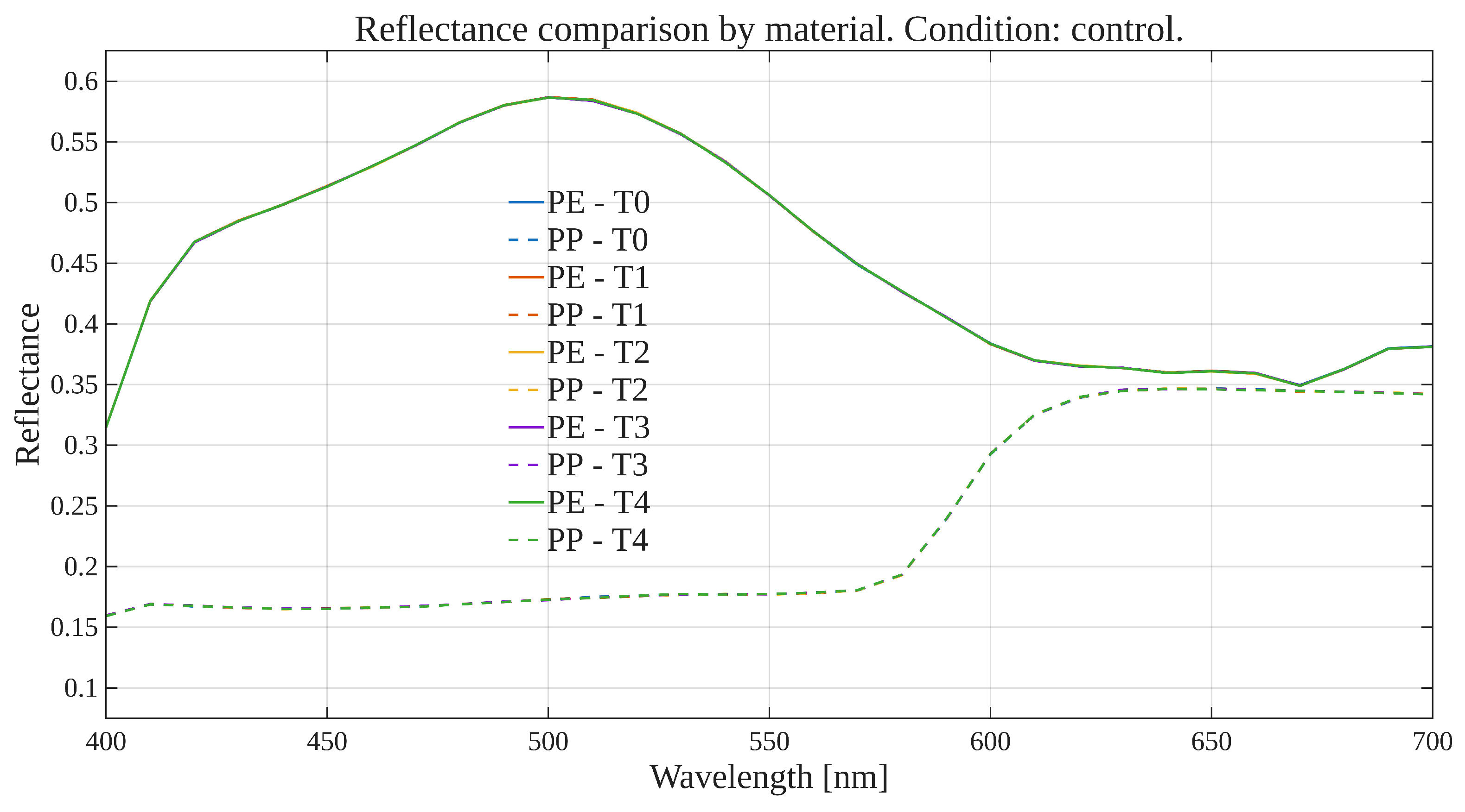
Mean reflectance curves for both polyethylene (solid lines) and polypropylene (dashed lines) under the control condition. One curve per time point (T0–T4).
Figure 1.
Mean reflectance curves for both polyethylene (solid lines) and polypropylene (dashed lines) under the control condition. One curve per time point (T0–T4).
Figure 2.
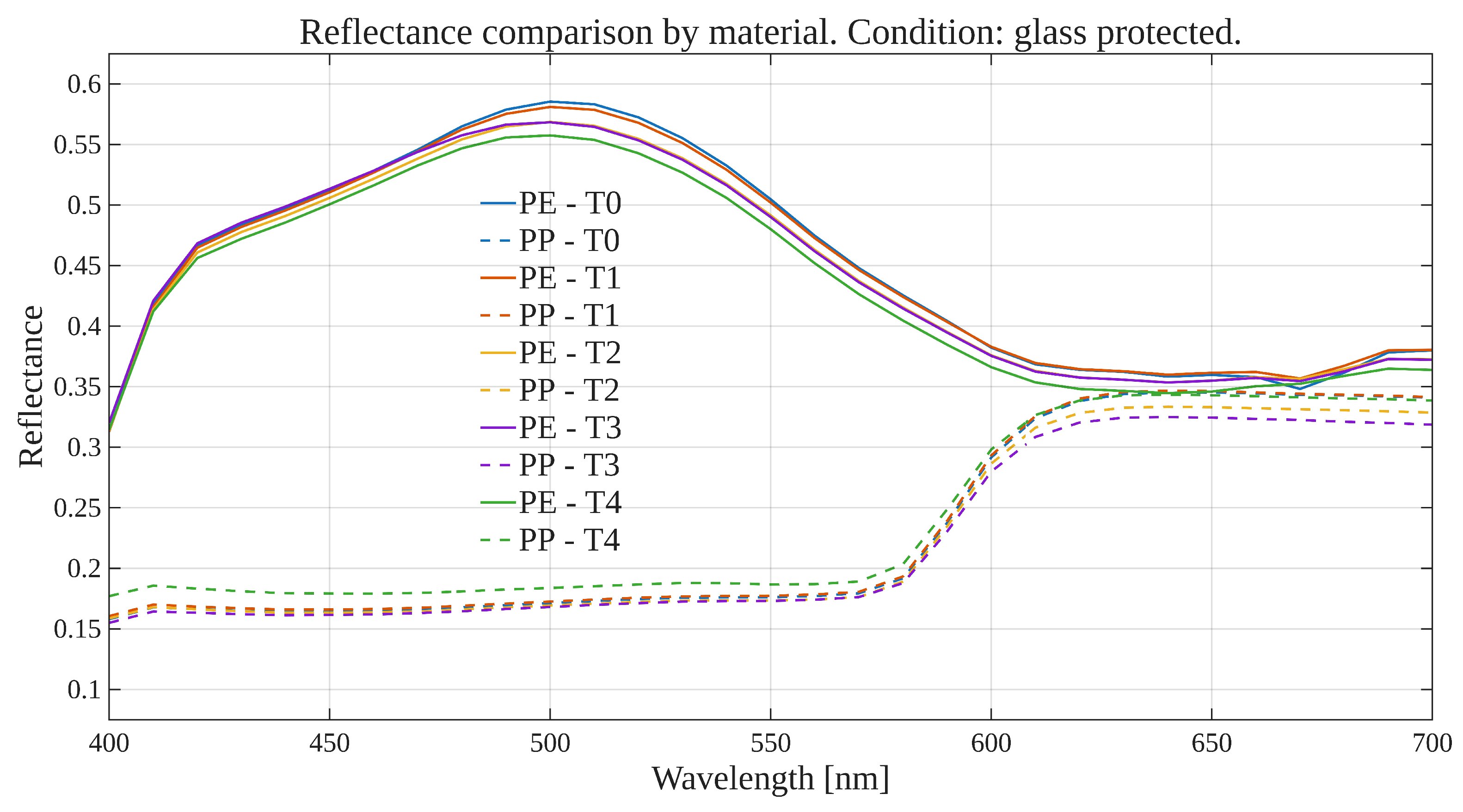
Mean reflectance curves for both polyethylene (solid lines) and polypropylene (dashed lines) under the glass-protected condition. One curve per time point (T0–T4).
Figure 2.
Mean reflectance curves for both polyethylene (solid lines) and polypropylene (dashed lines) under the glass-protected condition. One curve per time point (T0–T4).
Figure 3.
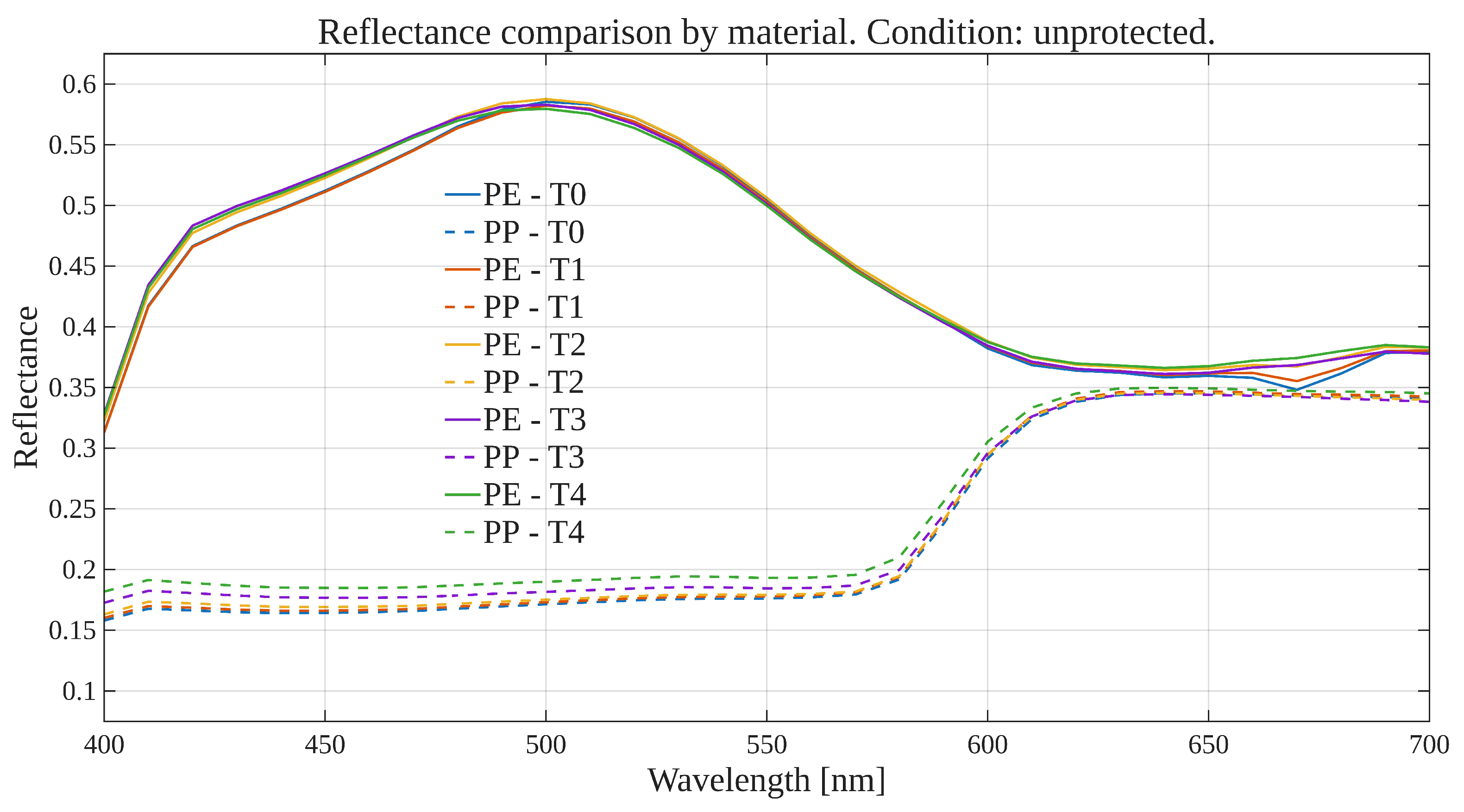
Mean reflectance curves for both polyethylene (solid lines) and polypropylene (dashed lines) under the unprotected condition (no glass coverage). One curve per time point (T0–T4).
Figure 3.
Mean reflectance curves for both polyethylene (solid lines) and polypropylene (dashed lines) under the unprotected condition (no glass coverage). One curve per time point (T0–T4).
Figure 4.
Mean reflectance curves for both polyethylene (solid lines) and polypropylene (dashed lines) under the UV chamber condition (ASTM G154 protocol). One curve per time point (T0–T4).
Figure 4.
Mean reflectance curves for both polyethylene (solid lines) and polypropylene (dashed lines) under the UV chamber condition (ASTM G154 protocol). One curve per time point (T0–T4).
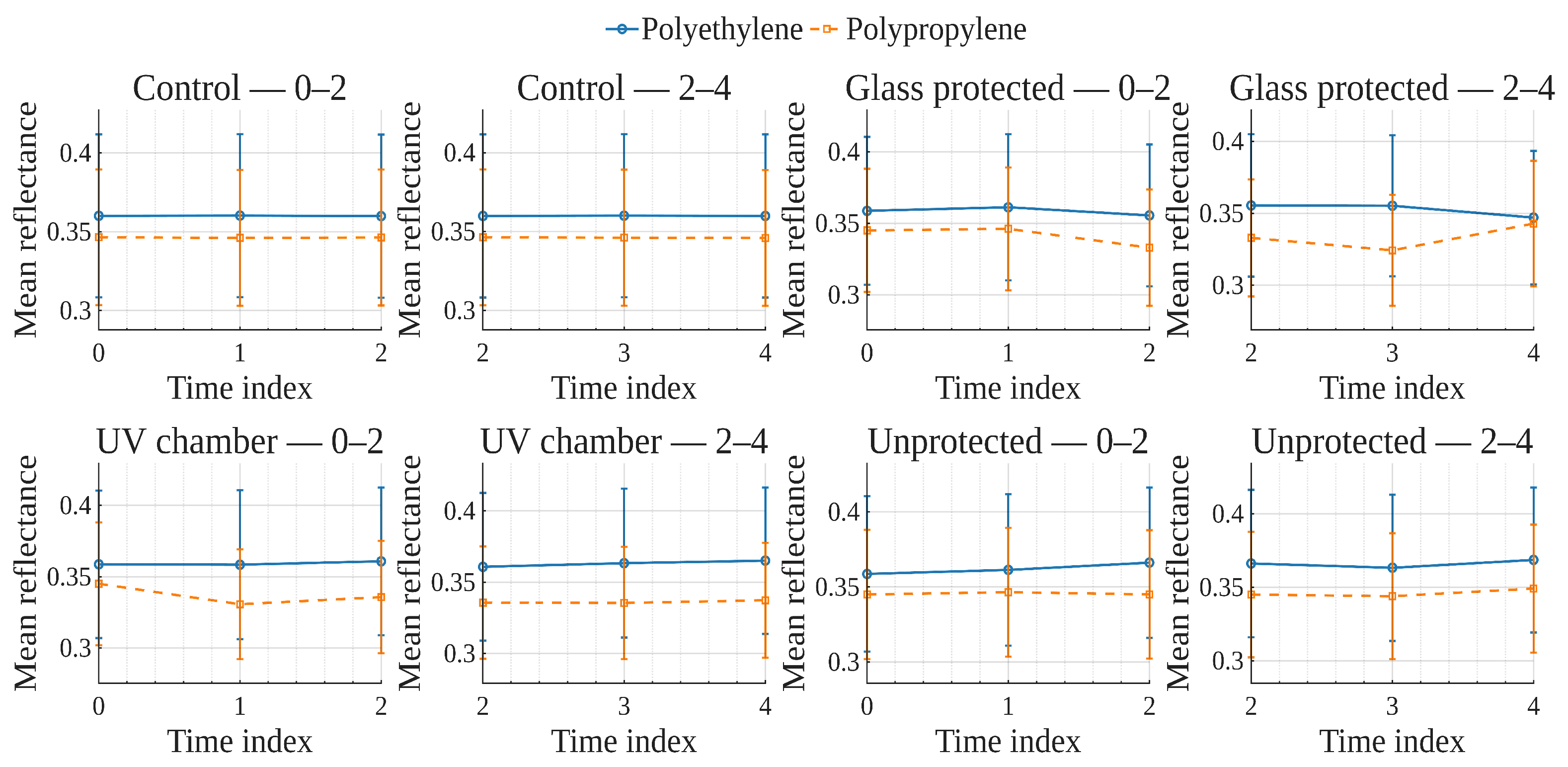
Figure 5.
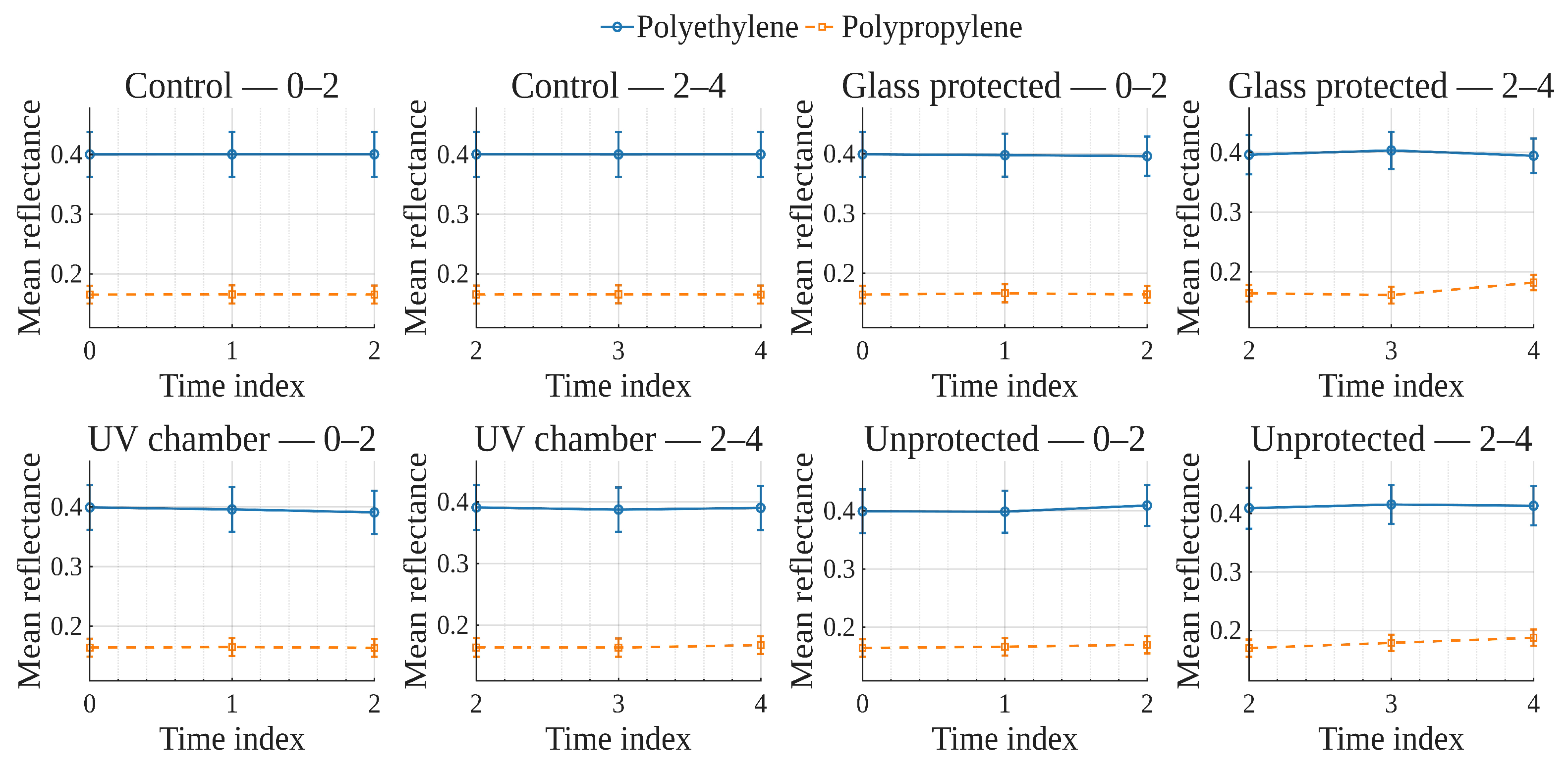
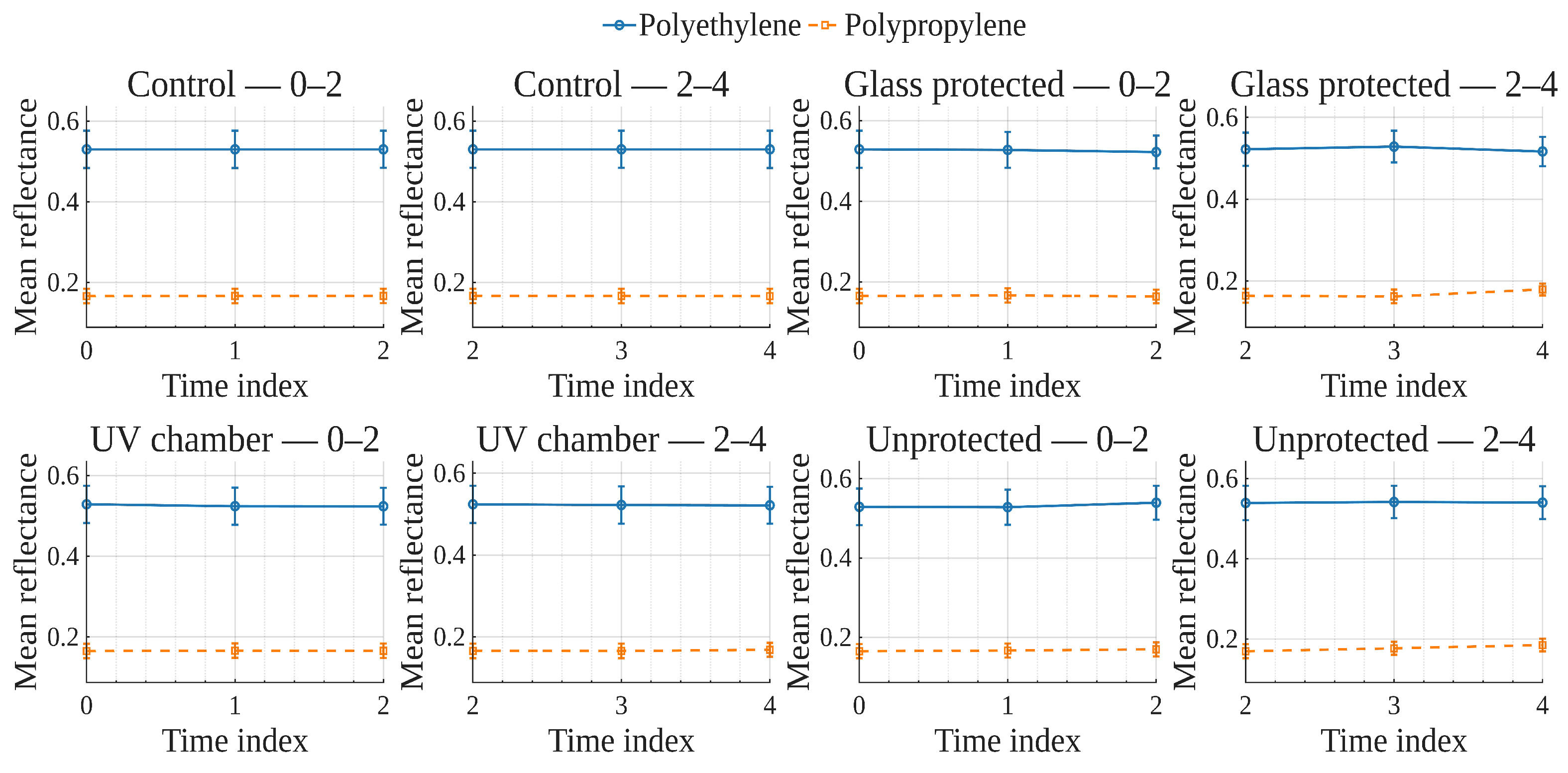
Temporal evolution of mean reflectance in the Violet band (400–420 nm) for polyethylene (solid lines) and polypropylene (dashed lines) under four conditions (Control, Glass-protected, Unprotected, and UV chamber). Panels split the time course into early (0–2) and late (2–4) intervals; markers denote integer times (T0–T4). Error bars show visually scaled (×0.30) SEM—standard error of the mean—applied uniformly across panels.
Figure 6.
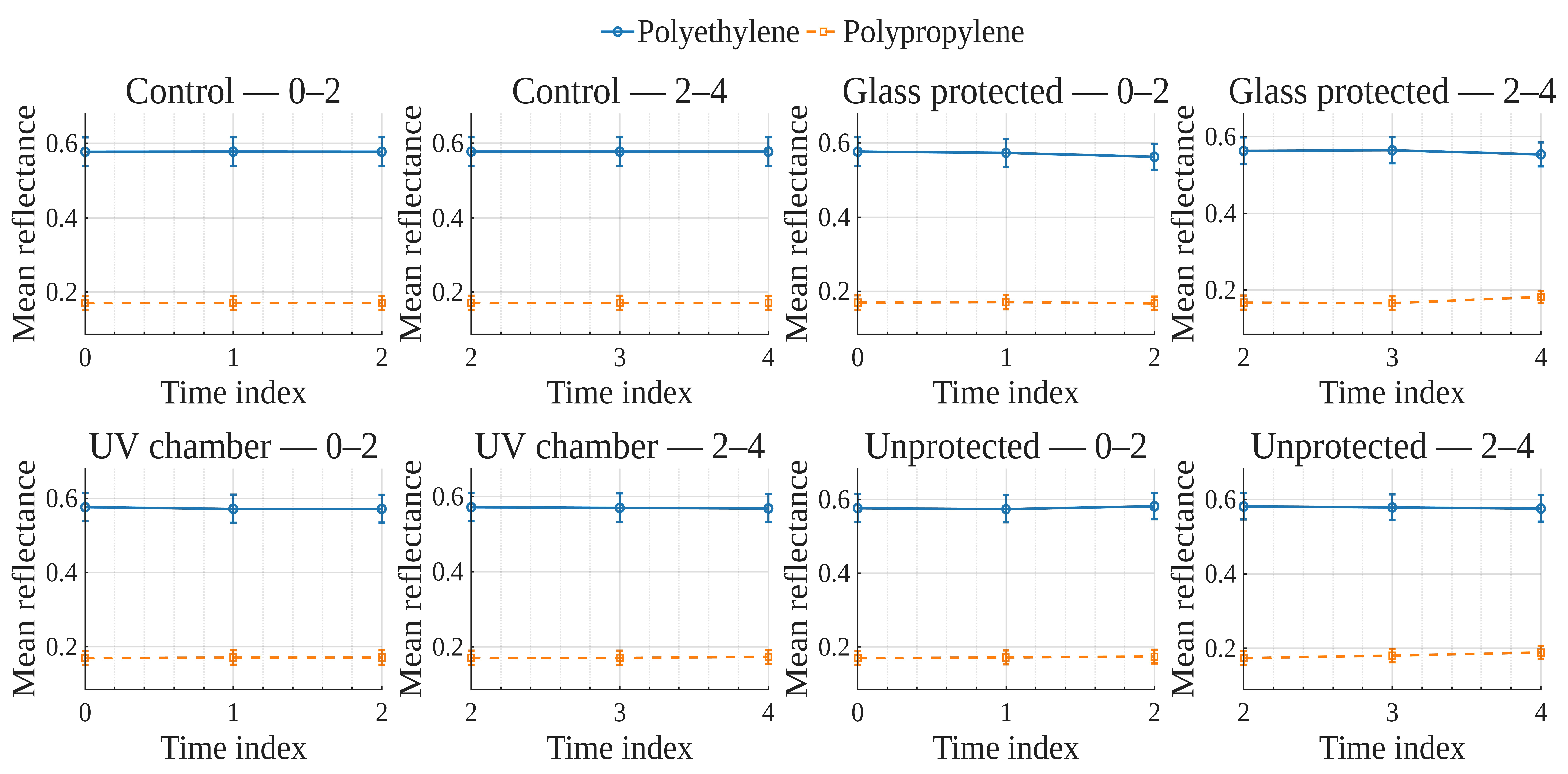
Temporal evolution of mean reflectance in the Blue band (450–470 nm) for polyethylene (solid) and polypropylene (dashed) across the four conditions (Control, Glass-protected, Unprotected, and UV chamber). Panels split the time course into early (0–2) and late (2–4) intervals; markers denote integer times (T0–T4). Error bars show visually scaled (×0.30) SEM—standard error of the mean—applied uniformly across panels.
Figure 7.
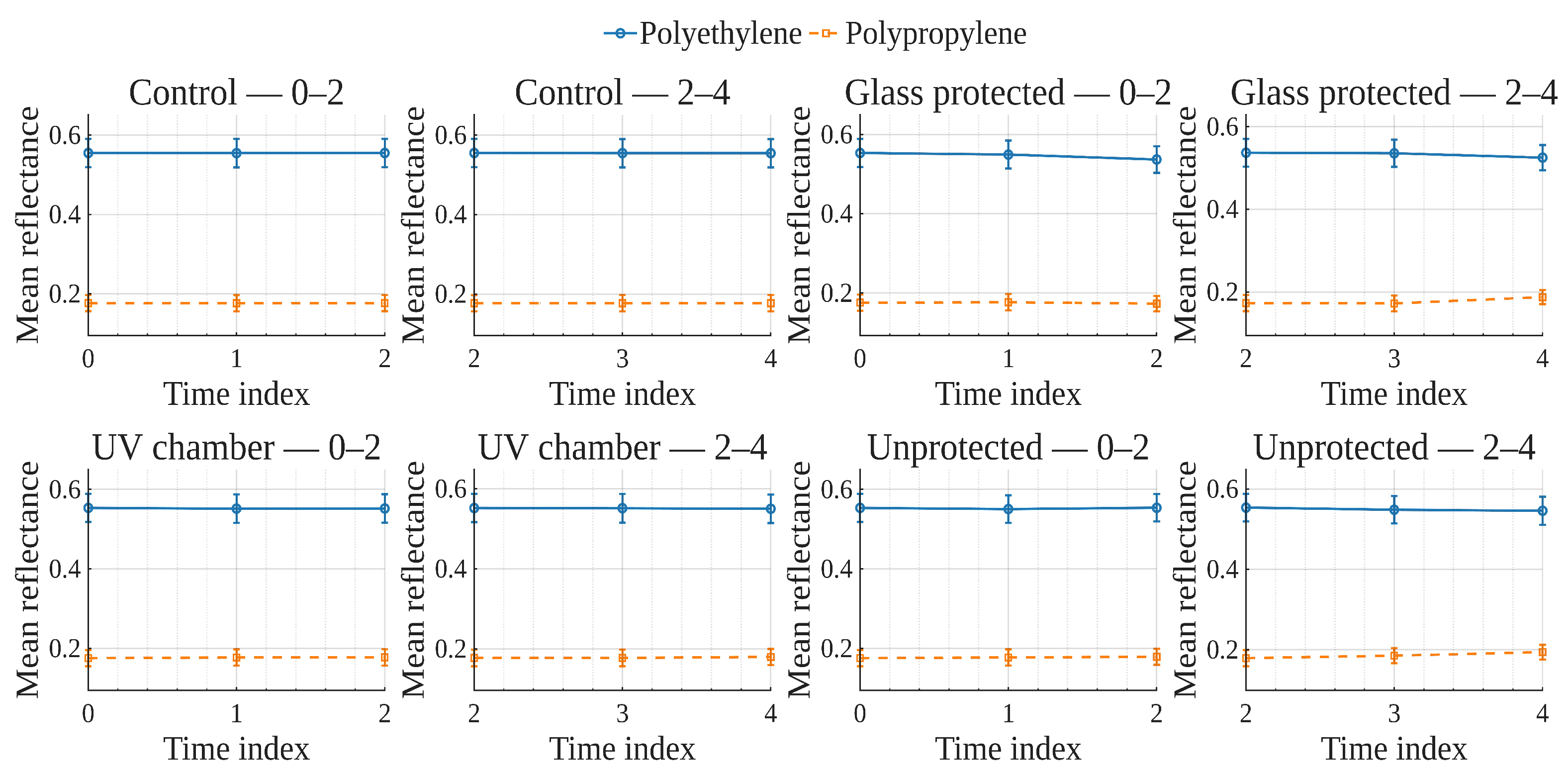
Temporal evolution of mean reflectance in the Cyan band (480–500 nm) comparing polyethylene (solid) versus polypropylene (dashed) under Control, Glass-protected, Unprotected, and UV chamber conditions. Panels split the time course into early (0–2) and late (2–4) intervals; markers denote integer times (T0–T4). Error bars show visually scaled (×0.30) SEM—standard error of the mean—applied uniformly across panels.
Figure 8.
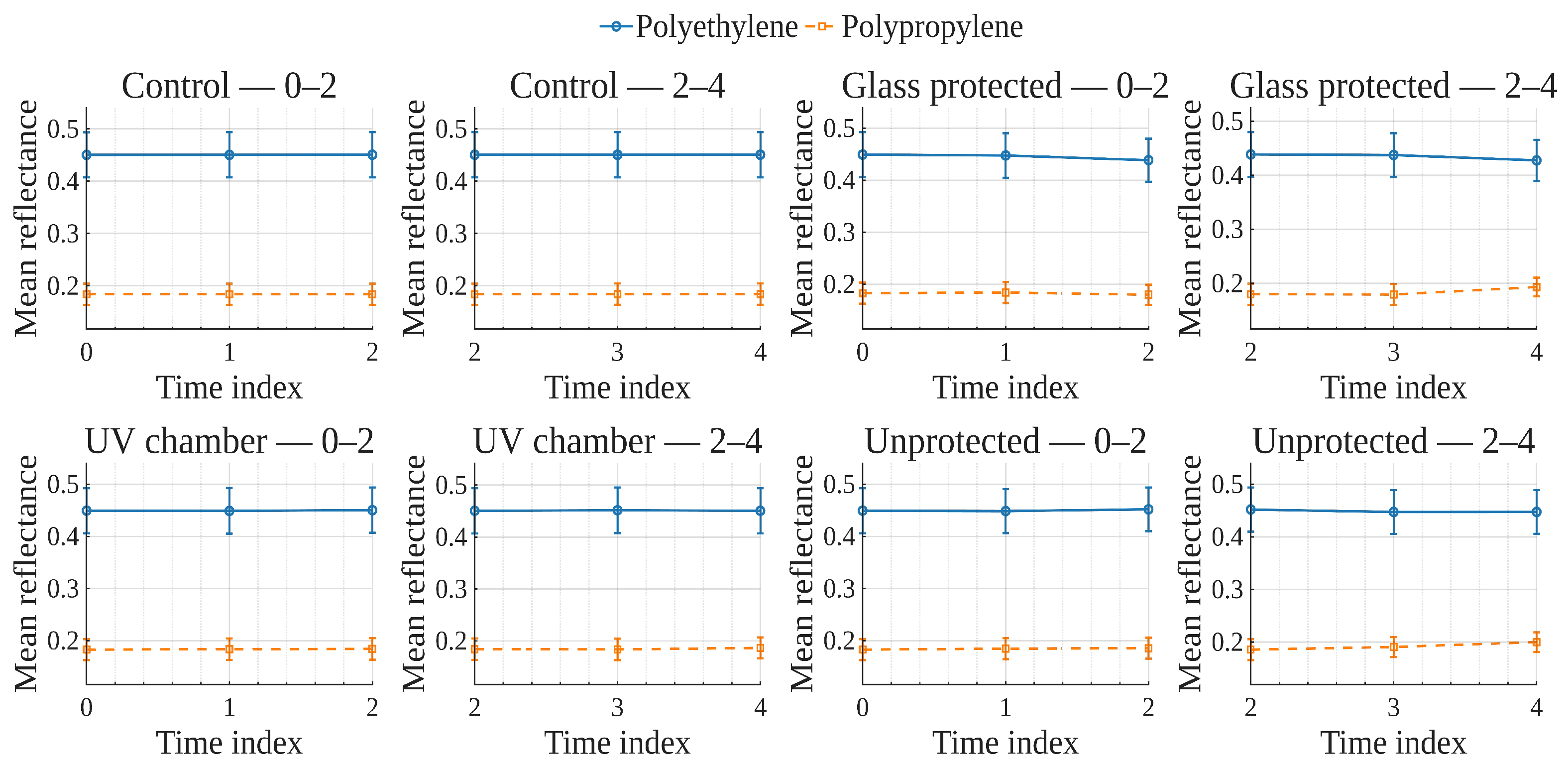
Temporal evolution of mean reflectance in the Green band (520–540 nm) for polyethylene (solid) and polypropylene (dashed) under the four illumination/exposure conditions. Panels split the time course into early (0–2) and late (2–4) intervals; markers denote integer times (T0–T4). Error bars show visually scaled (×0.30) SEM—standard error of the mean—applied uniformly across panels.
Figure 9.
Temporal evolution of mean reflectance in the Yellow band (560–580 nm) for polyethylene (solid) and polypropylene (dashed), by condition (Control, Glass-protected, Unprotected, and UV chamber). Panels split the time course into early (0–2) and late (2–4) intervals; markers denote integer times (T0–T4). Error bars show visually scaled (×0.30) SEM—standard error of the mean—applied uniformly across panels.
Figure 10.
Temporal evolution of mean reflectance in the Orange band (600–620 nm) for polyethylene (solid) versus polypropylene (dashed), shown per condition. Time segmentation (0–2 vs. 2–4) and scaled (×0.30) SEM—standard error of the mean bars.
Figure 10.
Temporal evolution of mean reflectance in the Orange band (600–620 nm) for polyethylene (solid) versus polypropylene (dashed), shown per condition. Time segmentation (0–2 vs. 2–4) and scaled (×0.30) SEM—standard error of the mean bars.
Figure 11.
Temporal evolution of mean reflectance in the Red band (640–660 nm) contrasting polyethylene (solid) and polypropylene (dashed) under Control, Glass-protected, Unprotected, and UV chamber conditions. Panels: 0–2 and 2–4; intervals: markers at integer times. Error bars: scaled SEM (×0.30) applied uniformly across bands and conditions.
Figure 12.
Subject-normalized degradation efficiency for polyethylene computed from spectral reflectance as , and then averaged across specimens within each condition (markers show group mean; error bars denote ±SD). Dashed curves are the best exponential fits selected by AICc among the candidate family (first-order, stretched, lag/offset variants, and bi-exponential). Time is shown as the discrete sampling index (–).
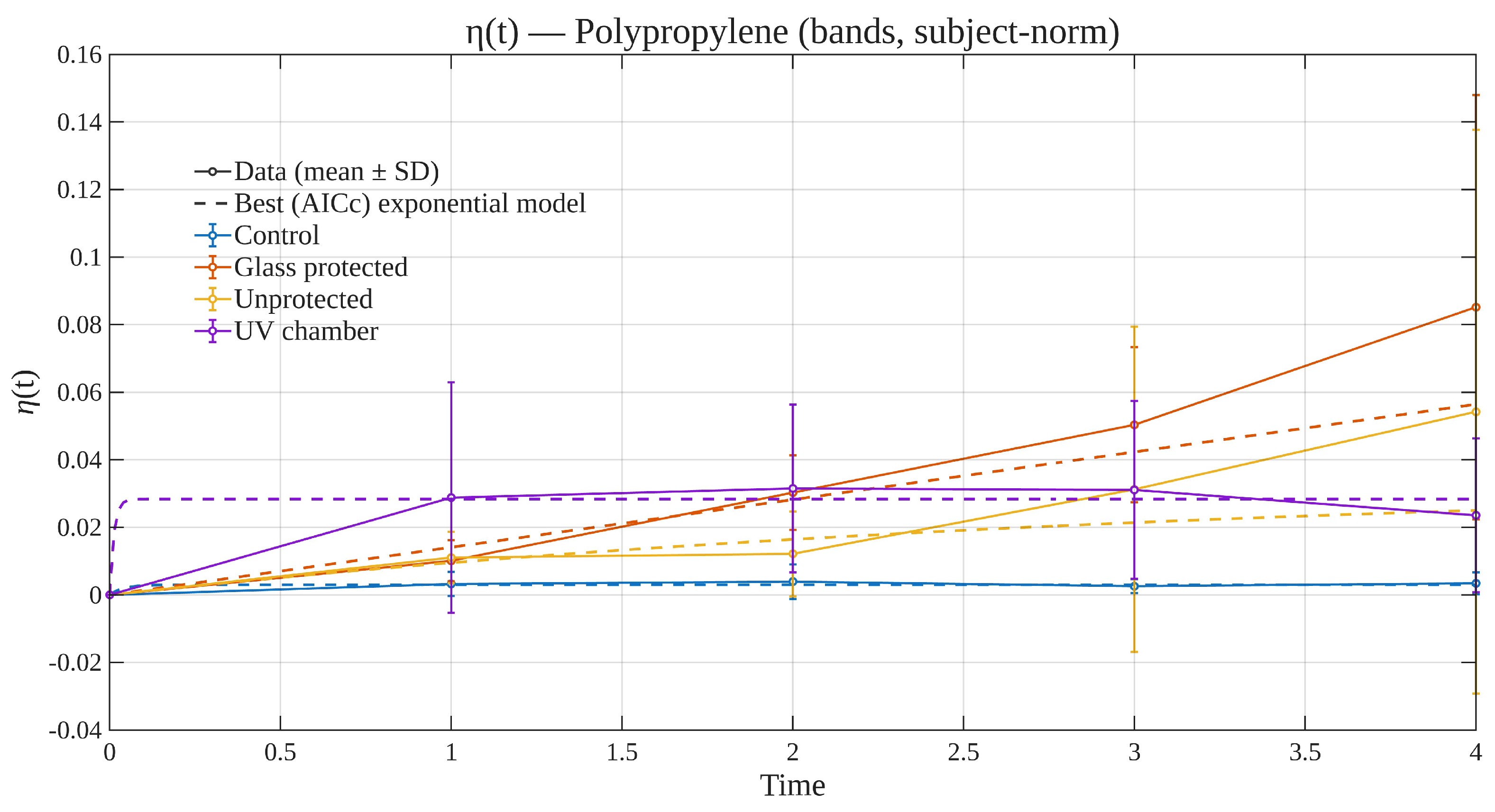
Figure 13.
Subject-normalized degradation efficiency for polypropylene under the four exposure conditions (mean ± SD across specimens). Dashed lines indicate the AICc-selected best exponential model in each condition. Time is the discrete sampling index (–).
Figure 13.
Subject-normalized degradation efficiency for polypropylene under the four exposure conditions (mean ± SD across specimens). Dashed lines indicate the AICc-selected best exponential model in each condition. Time is the discrete sampling index (–).
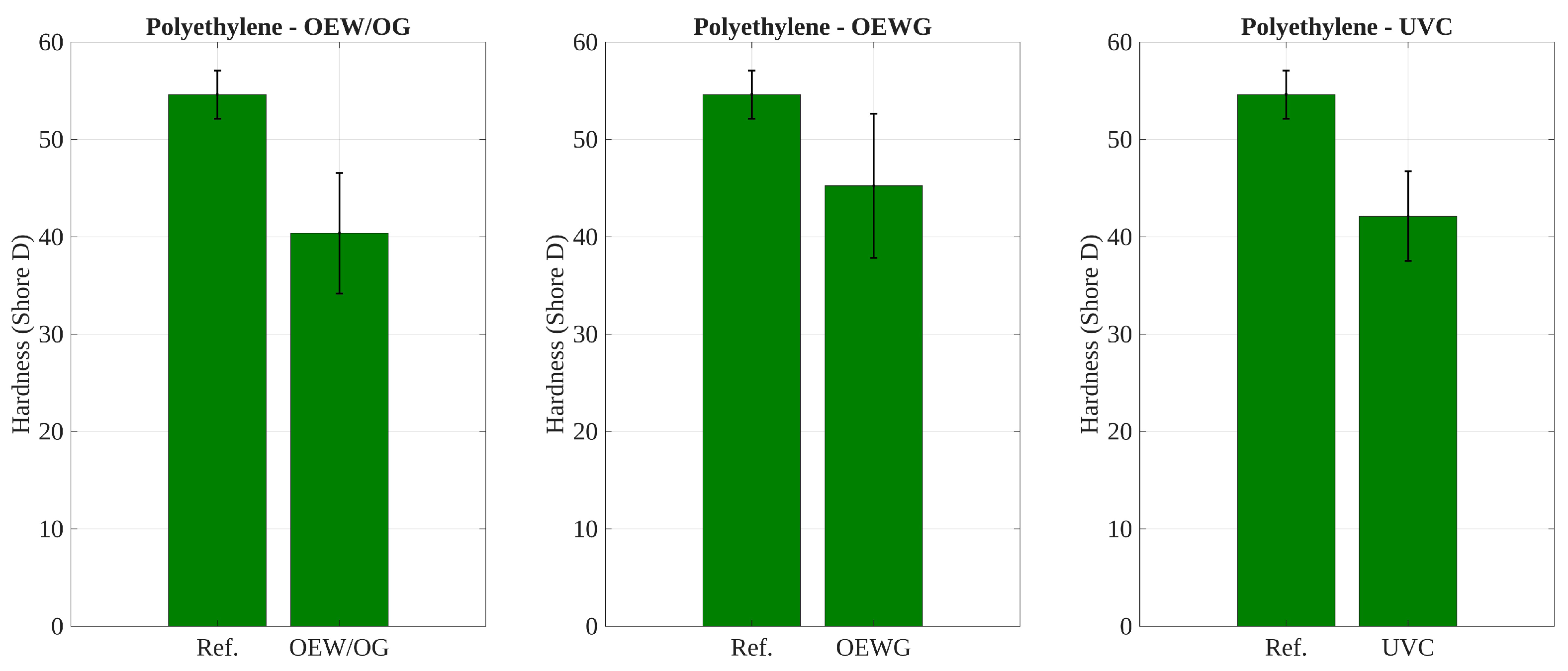
Figure 14.
Hardness comparison for polyethylene components before and after exposure. Bar plots show mean Shore D hardness with standard deviation. Three exposure conditions are compared against the reference: OEW/OG (open environment without glass), OEWG (open environment with glass), and UVC (simulated ultraviolet exposure). Significant differences are highlighted from pairwise tests.
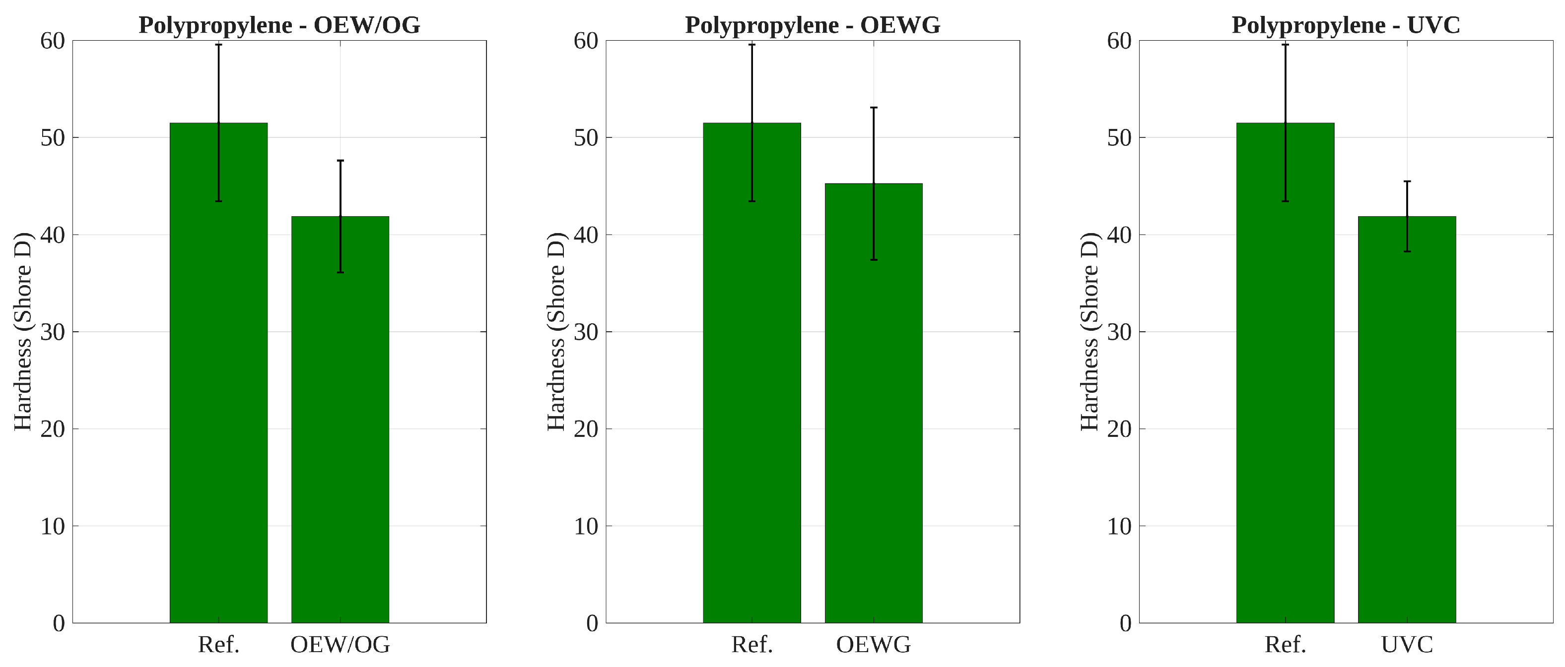
Figure 15.
Hardness comparison for polyethylene components before and after exposure. Bar plots show mean Shore D hardness with standard deviation. Three exposure conditions are compared against the reference: OEW/OG (open environment without glass), OEWG (open environment with glass), and UVC (simulated ultraviolet exposure). Significant differences are highlighted from pairwise tests.
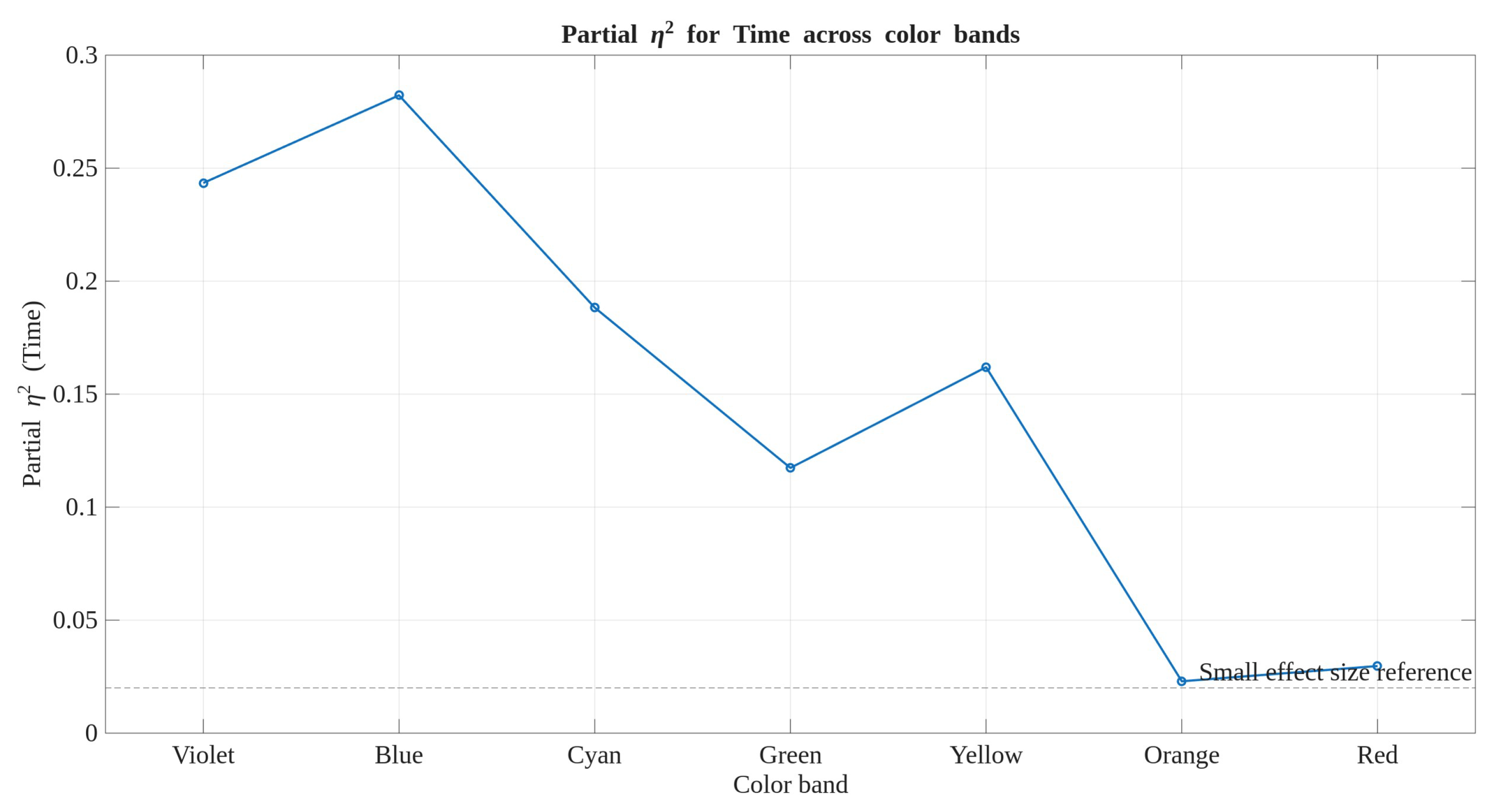
Figure 16.
(partial effect size) for the Time factor across VIS-bands. Values were obtained from repeated-measures ANCOVA adjusted for the baseline (T0) reflectance of each band, with Material and Condition as between-subject factors. The dashed horizontal line marks the threshold for a small effect size (). Error bars are omitted for clarity.
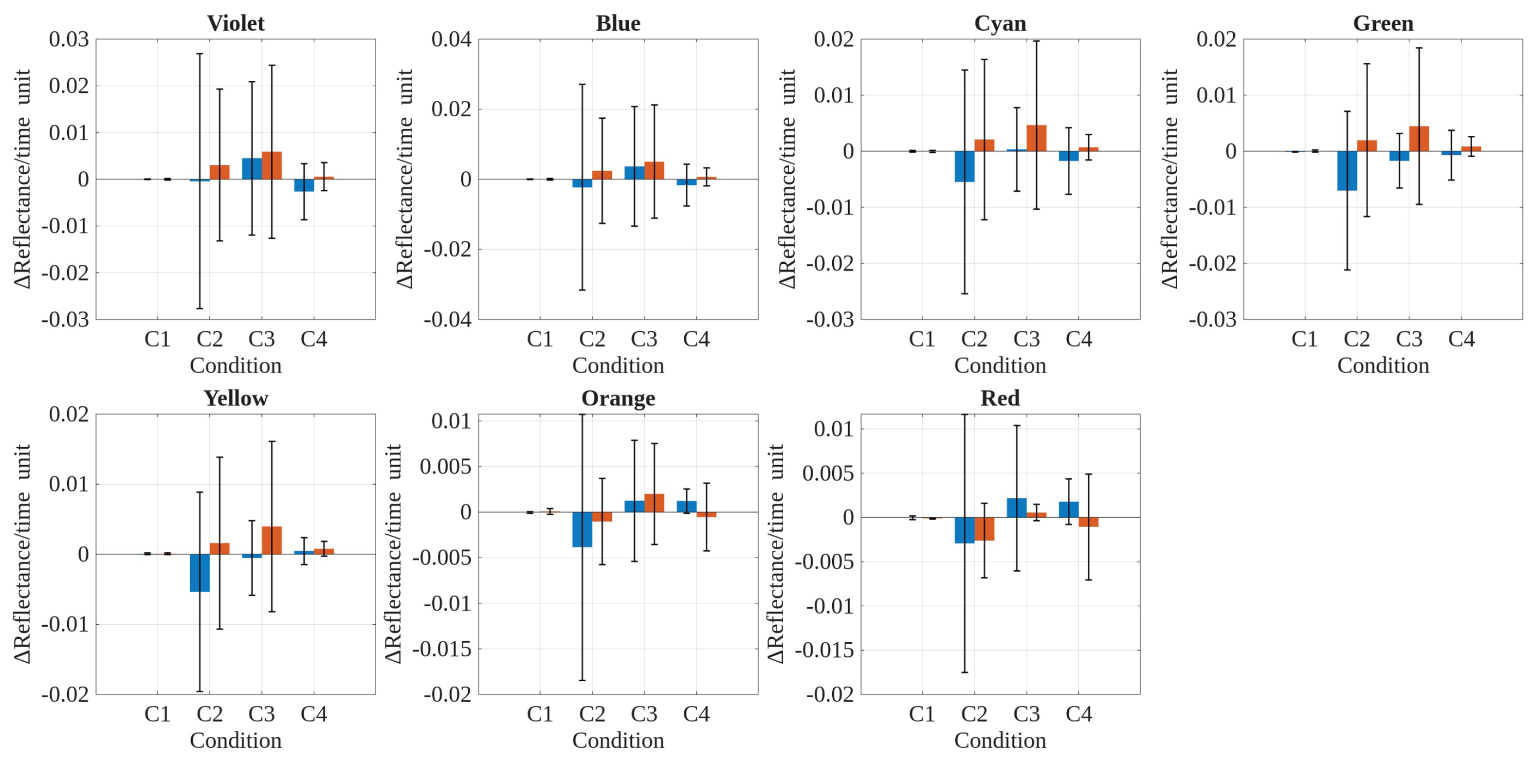
Figure 17.
Mean reflectance slopes with respect to time (i.e., Reflectance/time unit) for each VIS-band, comparing polyethylene (PE) and polypropylene (PP) under the four exposure conditions (C1–C4). Bars represent the group mean, and error bars indicate the standard deviation across replicates.
Figure 17.
Mean reflectance slopes with respect to time (i.e., Reflectance/time unit) for each VIS-band, comparing polyethylene (PE) and polypropylene (PP) under the four exposure conditions (C1–C4). Bars represent the group mean, and error bars indicate the standard deviation across replicates.
Table 1.
Features of the Gain Express Holdings Ltd. 560-10D Shore D digital durometer used.
Table 1.
Features of the Gain Express Holdings Ltd. 560-10D Shore D digital durometer used.
| Feature | Description |
|---|
| Sharp cone point | SR 0.1 [mm], 30° including angle. |
| Measure sample thickness | >6 [mm] (no more than 3 layers). |
| Measured area | Not less than the pressure edge of 15 [mm]. |
| LCD display | 4 digits, 40 × 18 [mm] (1.57×) 0.71 [inch]. |
| Measuring range/Graduation | 0–100 HD. |
| Indentor running | 0–2.2 [mm]. |
| Indentor press on telos | A, C type 0.55–8.06 [N], D type 0–44.5 [N]. |
| Resolution | 0.5 HD. |
| Power supply | 1 × SR44 button cell battery. |
| Item size | 87 [mm] × 56 [mm] × 25 [mm] (L × W × D) (3.43″ × 2.2″ × 0.98″) |
| Item weight | 36 [g] (4.79 [oz]). |
Table 2.
Features of the Konica Minolta CM-700d spectrophotometer used.
Table 2.
Features of the Konica Minolta CM-700d spectrophotometer used.
| Feature | Description |
|---|
| Illumination/viewing system | Diffused illumination, 8° viewing angle. |
| Specular component included/excluded. |
| Conforms to CIE No. 15 ISO 7724/1, DIN5033 Teil7, |
| ASTM E 1164, and JIS Z 8722. |
| Size of integrating sphere/diameter | 40 [mm]. |
| Spectral separation device | Diffraction grating. |
| Wavelength range | 400 to 700 [nm]. |
| Wavelength pitch | 10 [nm]. |
| Half bandwidth | ≃10 [nm]. |
| Reflectance range | 0 to 175%, display resolution: 0.01% |
| Light source | Pulsed Xenon Lamp (with UV cut filter). |
| Measurement time | ≃1 [s]. |
| Minimum measurement interval | ≃2 [s] (in SCI or SCE mode). |
Table 3.
Representative literature on polyolefin degradation quantification contrasted with the present VIS–reflectance framework. Prior work mostly quantifies damage via chemical or color indices (e.g., carbonyl index, yellowness), gas evolution, or mechanical retention; here, we use band-aggregated visible reflectance tracked over time and visualize a bounded, model-based trajectory as a compact descriptor of spectral change. Kinetic constants (, ) are discussed conceptually but are not tabulated in this version. Metrics and models are as reported by each source.
| Study | Material(s) | Illumination/Exposure | Metric (Proxy) | Reported Kinetics/ Key Outcome |
|---|
| Gulmine et al. (2003) [35] | PE (LDPE) | Artificial accelerated weathering | FTIR carbonyl index; UV-VIS; morphology | CI increases with dose; qualitative kinetics; links spectral growth to surface oxidation. |
| Fernando et al. (2007) [49] | PE, PP | Photodegradation (UV) | CO2 evolution; CI | Oxidation/gas-evolution correlates with CI; effective first-order-like regimes discussed. |
| Shyichuk et al. (2005) [57] | PE, PP, E–P copolymer | UV exposure; depth profiles | Depth-resolved CI | Near-surface oxidation dominates; gradients consistent with short- absorption, implicit multi-timescale behavior. |
| Tocháček & Vrátničková (2014) [17] | PP and copolymers | UV accelerated; temperature effects | Mechanical retention; color/CI | Temperature accelerates damage; Arrhenius-type behavior; practical lifetime prediction. |
| Rodríguez et al. (2020) [8] | LDPE | UV-aging | Tensile/fracture metrics | Monotonic loss of toughness; time-to-threshold comparisons; no explicit spectral efficiency. |
| Grause et al. (2020) [58] | LDPE, HDPE, PP | Natural/outdoor and accelerated UV weathering (survey across setups) | FTIR, UV-VIS, DSC, mechanical testing | Carbonyl Index (CI), yellowness index, crystallinity increase, tensile retention. |
| Bourgogne et al. (2022) [44] | Polymers (incl. polyolefins context) | LED weathering, wavelength-resolved | Chemical/CI changes | Shorter wavelengths drive faster photooxidation; wavelength selectivity highlighted. |
| Du et al. (2024) [21] | PE sheets (types) | UV; varied parameters | Multi-technique spectral/material indices | Factor sensitivity (grade, thickness, stabilizers); qualitative kinetics under parameter sweeps. |
| Arese et al. (2025) [3] | Recycled PP | UV ageing | Morphological, thermal, mechanical | Stabilization/processing history modulate ageing; no unified bounded spectral metric. |
| This work | PE, PP | VIS: unprotected vs. glass-protected; UV chamber | Band-aggregated VIS reflectance (7 bands; full spectrum inspected); visualized | Compact, model-based spectral trajectories selected by small-sample information criteria; graphical comparison across materials/conditions/bands; kinetic constants discussion. |
Table 4.
Statistical analysis summary of Shore D hardness measurements for polyethylene and polypropylene samples before and after environmental exposure. Paired tests (parametric or nonparametric depending on normality) compared each post-exposure condition to the reference (unexposed, reference hardness, i.e., RH) state. Complementarily, a one-way ANOVA with Tukey’s post hoc comparisons was conducted separately for each material to assess overall differences across exposure conditions. Each result indicates whether the difference was statistically significant at the level.
| Material | Test Type | Results |
|---|
| Polyethylene | Paired comparisons (vs. RH) | Outdoor exposure without glass (OEW/OG):
Outdoor exposure with glass (OEWG):
Simulated UV chamber (UVC): |
| One-way ANOVA + Tukey | Global test:
Significant differences: RH-OEW/OG, RH-UVC |
| Polypropylene | Paired comparisons (vs. RH) | Outdoor exposure without glass (OEW/OG):
Outdoor exposure with glass (OEWG):
Simulated UV chamber (UVC): |
| One-way ANOVA + Tukey | Global test:
Significant differences: RH-OEW/OG, RH-OEWG, RH-UVC |
Table 5.
ANCOVA significance summary for mean reflectance in each visible VIS-band. The model includes Material (polyethylene or polypropylene), Condition (four environmental exposure scenarios), Time (T1–T4), and the covariate initial reflectance measured at T0. All main effects and interaction terms up to the four-way level were tested. Cells indicate whether each effect was statistically significant () or not (). This full-factorial model controls for initial reflectance differences and evaluates the extent to which reflectance changes depend on material type, exposure conditions, and time.
| VIS-Band | Material | Condition | Time | Covariate | M × C | M × T | M × Cov | C × T | C × Cov | T × Cov | M × C × T | M × C × Cov | M × T × Cov | C × T × Cov | M × C × T × Cov |
|---|
| Violet | | | | | | | | | | | | | | | |
| Blue | | | | | | | | | | | | | | | |
| Cyan | | | | | | | | | | | | | | | |
| Green | | | | | | | | | | | | | | | |
| Yellow | | | | | | | | | | | | | | | |
| Orange | | | | | | | | | | | | | | | |
| Red | | | | | | | | | | | | | | | |
Table 6.
Two-way ANOVA (p values) evaluating the effects of exposure Condition (C1: no exposure, C2: exposure under glass, C3: exposure without glass, C4: artificial UV exposure; ASTM G154 protocol), Time (T0 to T4), and their interaction on the average visible reflectance of automotive plastic specimens. The response variable is the mean reflectance within each visible VIS-band, calculated as the average reflectance over three adjacent wavelengths for each VIS-band (Violet to Red). The analysis was conducted separately for each material: polyethylene (PE) and polypropylene (PP). Each cell indicates whether the effect was statistically significant at the level.
| Color | PE Cond | PE Time | PE Cond × Time | PP Cond | PP Time | PP Cond × Time |
|---|
| Violet | p > 0.05 | p > 0.05 | p > 0.05 | p > 0.05 | p > 0.05 | p > 0.05 |
| Blue | p > 0.05 | p > 0.05 | p > 0.05 | p > 0.05 | p > 0.05 | p > 0.05 |
| Cyan | p > 0.05 | p > 0.05 | p > 0.05 | p > 0.05 | p > 0.05 | p > 0.05 |
| Green | p > 0.05 | p > 0.05 | p > 0.05 | p > 0.05 | p > 0.05 | p > 0.05 |
| Yellow | p > 0.05 | p > 0.05 | p > 0.05 | p > 0.05 | p > 0.05 | p > 0.05 |
| Orange | p > 0.05 | p > 0.05 | p > 0.05 | p > 0.05 | p > 0.05 | p > 0.05 |
| Red | p > 0.05 | p > 0.05 | p > 0.05 | p > 0.05 | p > 0.05 | p > 0.05 |
Table 7.
ANCOVA significance summary for average reflectance in each visible VIS-band, analyzed separately for polyethylene and polypropylene. Each model included the fixed factors Condition (four environmental exposure scenarios) and Time (four sampling points: to ), as well as the covariate Initial Reflectance measured at baseline (). All second-order interactions (Condition × Time, Condition × Covariate, Time × Covariate) and the third-order interaction (Condition × Time × Covariate) were also tested. The table reports whether each effect was statistically significant () or not (), based on individual ANCOVA models fitted for each visible VIS-band.
| Material | VIS-Band | Condition | Time | Covariate | C × T | C × Cov | T × Cov | C × T × Cov |
|---|
| Polyethylene | Violet | | | | | | | |
| Polyethylene | Blue | | | | | | | |
| Polyethylene | Cyan | | | | | | | |
| Polyethylene | Green | | | | | | | |
| Polyethylene | Yellow | | | | | | | |
| Polyethylene | Orange | | | | | | | |
| Polyethylene | Red | | | | | | | |
| Polypropylene | Violet | | | | | | | |
| Polypropylene | Blue | | | | | | | |
| Polypropylene | Cyan | | | | | | | |
| Polypropylene | Green | | | | | | | |
| Polypropylene | Yellow | | | | | | | |
| Polypropylene | Orange | | | | | | | |
| Polypropylene | Red | | | | | | | |
Table 8.
Multivariate analysis of variance (MANOVA) assessing the effects of Material (polyethylene, polypropylene), Condition (C1: no exposure; C2: environmental exposure under glass; C3: environmental exposure without protection; C4: UV chamber, ASTM G154 protocol), Time (T0 to T4), and their interactions on the multivariate response of average spectral reflectance. The table summarizes the statistical significance of each factor and interaction across four multivariate test statistics: Wilks’s , Pillai’s trace, Hotelling–Lawley trace, and Roy’s greatest root.
| Effect | Test | Significance |
|---|
| Material | Wilks’s | |
| Pillai’s trace | |
| Hotelling–Lawley trace | |
| Roy’s greatest root | |
| Condition | Wilks’s | |
| Pillai’s trace | |
| Hotelling–Lawley trace | |
| Roy’s greatest root | |
| Time | Wilks’s | |
| Pillai’s trace | |
| Hotelling–Lawley trace | |
| Roy’s greatest root | |
| Material × Condition | Wilks’s | |
| Pillai’s trace | |
| Hotelling–Lawley trace | |
| Roy’s greatest root | |
| Material × Time | Wilks’s | |
| Pillai’s trace | |
| Hotelling–Lawley trace | |
| Roy’s greatest root | |
| Condition × Time | Wilks’s | |
| Pillai’s trace | |
| Hotelling–Lawley trace | |
| Roy’s greatest root | |
| Material × Condition × Time | Wilks’s | |
| Pillai’s trace | |
| Hotelling–Lawley trace | |
| Roy’s greatest root | |
Table 9.
Multivariate significance summary from a MANCOVA model adjusted by initial reflectance (T0) for each average visible VIS-band. The response matrix includes the average reflectance values for seven spectral bands (Violet, Blue, Cyan, Green, Yellow, Orange, and Red) across 224 observations. The model tests the main effects of Material (polyethylene or polypropylene), Condition (four levels of environmental exposure), and Time (four sampling stages from T1 to T4), as well as second- and third-order interactions between these factors. Each cell indicates whether the corresponding effect was statistically or not according to four multivariate test statistics: Wilks’s , Pillai’s trace, Hotelling–Lawley trace, and Roy’s largest root.
| Effect | Wilks’s | Pillai’s Trace | Hotelling–Lawley | Roy’s Largest Root |
|---|
| Material | | | | |
| Condition | | | | |
| Time | | | | |
| Material × Condition | | | | |
| Material × Time | | | | |
| Condition × Time | | | | |
| Material × Condition × Time | | | | |
Table 10.
Multivariate analysis of variance (MANOVA) results for the repeated-measures effects of Condition, Time, and their interaction on the mean reflectance across seven visible VIS-bands (Violet to Red). The analysis was conducted separately for polyethylene and polypropylene samples. Each entry indicates whether the corresponding multivariate test (Wilks’s Lambda, Pillai’s Trace, Hotelling–Lawley Trace, Roy’s Greatest Root) yielded statistical significance () or not (). Both Condition and Time were treated as within-subjects factors in the repeated-measures design.
| Effect | Polyethylene | Polypropylene |
|---|
|
Wilks
|
Pillai
|
Hotelling
|
Roy
|
Wilks
|
Pillai
|
Hotelling
|
Roy
|
|---|
| Condition | | | | | | | | |
| Time | | | | | | | | |
| Condition × Time | | | | | | | | |
Table 11.
Multivariate significance summary from two separate MANCOVA models conducted for polyethylene and polypropylene, respectively. The response matrix consists of the average reflectance values computed for each of the seven visible VIS-bands measured at four post-exposure stages (T1 to T4). Each model includes two fixed between-subject factors: Condition (four levels of environmental exposure) and Time (T1 to T4), as well as their second-order interaction (Condition × Time). The initial reflectance (T0) was included as a covariate to control for baseline variability. Statistical significance ( or ) was evaluated using four classical multivariate test statistics: Wilks’s , Pillai’s trace, Hotelling–Lawley trace, and Roy’s largest root.
| Material | Effect | Wilks’s | Pillai’s Trace | Hotelling–Lawley Trace | Roy’s Largest Root |
|---|
| Polyethylene | Condition | | | | |
| Time | | | | |
| Condition × Time | | | | |
| Polypropylene | Condition | | | | |
| Time | | | | |
| Condition × Time | | | | |
Table 12.
ANOVA results (p values) for average reflectance per VIS-band, including the interaction between Material (M), Condition (C), and Time (T). Each cell indicates whether the effect was statistically significant at the level. Summary of significance thresholds (p values) from a three-way ANOVA performed on the average reflectance per VIS-band. The response variable is the mean reflectance computed for each band of the visible spectrum (Violet to Red), based on the average of three adjacent wavelengths. The between-subject factors considered are Material (polyethylene or polypropylene), Condition (four levels of environmental exposure), and Time (five measurement times). Each cell indicates whether the corresponding main effect or interaction was statistically significant at .
| Color | Material | Condition | Time | M × C | M × T | C × T | M × C × T |
|---|
| Violet | | | | | | | |
| Blue | | | | | | | |
| Cian | | | | | | | |
| Green | | | | | | | |
| Yellow | | | | | | | |
| Orange | | | | | | | |
| Red | | | | | | | |
