
Prediction and Interpretability Study of the Glass Transition Temperature of Polyimide Based on Machine Learning and Molecular Dynamics Simulations

Abstract
1. Introduction
2. Materials and Methods
2.1. Database and Feature Selection
2.2. Machine Learning Methods
2.3. Model Interpretation and Validation
3. Results
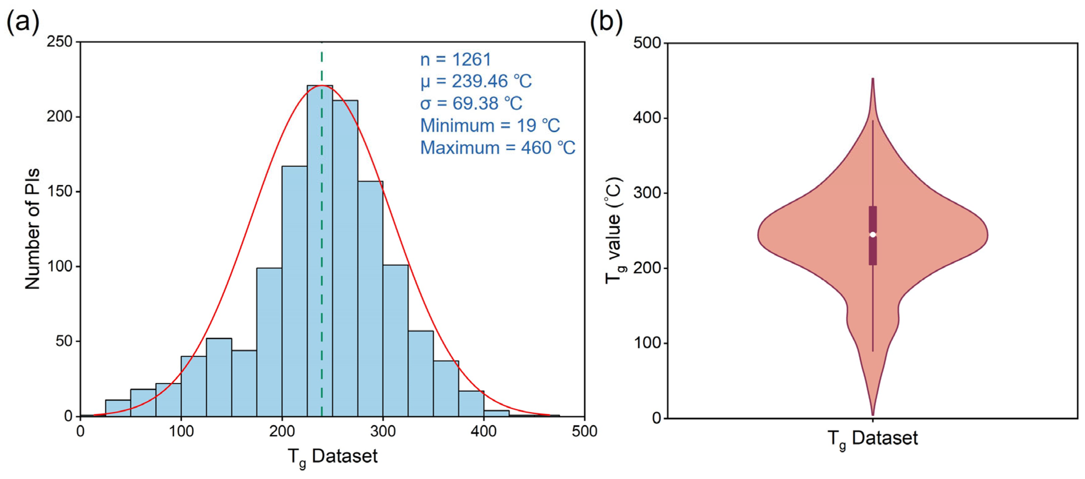
3.1. Data Collection and Feature Extraction
3.2. Performance Evaluation of the ML Models
3.3. Interpretability Analysis of the Model Using SHAP
3.4. MD Validation
4. Conclusions
Supplementary Materials
Author Contributions
Funding
Institutional Review Board Statement
Data Availability Statement
Conflicts of Interest
Abbreviations
| PI | polyimide |
| Tg | glass transition temperature |
| ML | machine learning |
| MD | molecular dynamics |
| QSPR | quantitative structure–property relationships |
| LASSO | Least Absolute Shrinkage and Selection Operator |
| XGB | eXtreme Gradient Boosting |
| ANN | Artificial Neural Network |
| DNN | Deep Neural Network |
| ET | Extra Trees |
| GBDT | Gradient Boosting Decision Tree |
| LGBM | Light Gradient Boosting Machine |
| AB | AdaBoost regression |
| CATB | Categorical Boosting |
| GPR | Gaussian Process Regression |
| R2 | coefficient of determination |
| MAE | mean absolute error |
| RMSE | root mean square error |
| SHAP | SHapley Additive exPlanations |
References
- Zhang, X.; Dou, Y.; Liu, L.; Song, M.; Xi, Z.; Xu, Y.; Shen, W.; Wang, J. Polyimide Films Based on β-Cyclodextrin Polyrotaxane with Low Dielectric and Excellent Comprehensive Performance. Polymers 2024, 16, 901. [Google Scholar] [CrossRef]
- Liu, Y.; Wang, Y.; Wu, D. Synthetic strategies for highly transparent and colorless polyimide film. J. Appl. Polym. Sci. 2022, 139, e52604. [Google Scholar] [CrossRef]
- Feng, J.; Wang, Y.; Qin, X.; Lv, Y.; Huang, Y.; Yang, Q.; Li, G.; Kong, M. Revealing molecular mechanisms of colorless transparent polyimide films under photo-oxidation. Polym. Degrad. Stab. 2023, 210, 110294. [Google Scholar] [CrossRef]
- Lian, M.; Tian, L.; Huang, G.; Liang, S.; Zhang, Y.; Yi, N.; Fan, L.; Wu, Q.; Gan, F.; Wu, Y. Recent Advances in Fluorescent Polyimides. Molecules 2024, 29, 4072. [Google Scholar] [CrossRef]
- Ren, X.; He, Z.; Wang, Z.; Pan, Z.; Qi, Y.; Han, S.; Yu, H.; Liu, J. Design, Synthesis and Properties of Semi-Alicyclic Colorless and Transparent Polyimide Films with High Glass Transition Temperatures and Low Retardation for Potential Applications in Flexible Electronics. Polymers 2023, 15, 3408. [Google Scholar] [CrossRef]
- Ghaffari-Mosanenzadeh, S.; Tafreshi, O.A.; Karamikamkar, S.; Saadatnia, Z.; Rad, E.; Meysami, M.; Naguib, H.E. Recent advances in tailoring and improving the properties of polyimide aerogels and their application. Adv. Colloid Interface Sci. 2022, 304, 102646. [Google Scholar] [CrossRef]
- Wan, B.; Dong, X.; Yang, X.; Wang, J.; Zheng, M.; Dang, Z.; Chen, G.; Zha, J. Rising of Dynamic Polyimide Materials: A Versatile Dielectric for Electrical and Electronic Applications. Adv. Mater. 2023, 35, 2301185. [Google Scholar] [CrossRef] [PubMed]
- Yan, X.; Wang, Y.; Yu, T.; Chen, H.; Zhao, Z.; Guan, S. Polyimide binder by combining with polyimide separator for enhancing the electrochemical performance of lithium ion batteries. Electrochim. Acta 2016, 216, 1–7. [Google Scholar] [CrossRef]
- Zhang, H.; Xiang, Z.; Fang, P.; Zang, S.; Zheng, Z. Soluble Polyimide-Modified Epoxy Resin with Enhanced Comprehensive Performances. J. Appl. Polym. Sci. 2025, e57400. [Google Scholar] [CrossRef]
- Lan, Y.; Xi, Y.; Xiong, W.; Liu, X.; Wang, Z.; Huang, S.; Lin, J.; Yin, C.; Li, X.; Zhou, L. The effect of temperature on the roll graphite films derived from Kapton polyimide films. Appl. Phys. A 2024, 130, 497. [Google Scholar] [CrossRef]
- Frazer, A.H. New linear polymers. Henry Lee, Donald Staffey and Rris Neville McGraw-Hill, New York, 1967. x + 374 pp, illus. J. Polym. Sci. Part A-1 1969, 7, 2464. [Google Scholar] [CrossRef]
- Gudla, H.; Zhang, C. How to Determine Glass Transition Temperature of Polymer Electrolytes from Molecular Dynamics Simulations. J. Phys. Chem. B 2024, 128, 10537–10540. [Google Scholar] [CrossRef]
- Tsai, C.L.; Yen, H.J.; Liou, G.S. Highly transparent polyimide hybrids for optoelectronic applications. React. Funct. Polym. 2016, 108, 2–30. [Google Scholar] [CrossRef]
- Luo, F.; Lin, C.; Jiao, L.; Du, Z.; Dong, Z.; Dai, X.; Duan, X.; Qiu, X. High glass transition temperature and ultra-low thermal expansion coefficient polyimide films containing rigid pyridine and bisbenzoxazole units. J. Polym. Sci. 2023, 61, 1289–1297. [Google Scholar] [CrossRef]
- Song, J.; Qin, H.; Qin, S.; Liu, M.; Zhang, S.; Chen, J.; Zhang, Y.; Wang, S.; Li, Q.; Dong, L.; et al. Alicyclic polyimides with large band gaps exhibit superior high-temperature capacitive energy storage. Mater. Horiz. 2023, 10, 2139–2148. [Google Scholar] [CrossRef] [PubMed]
- Costa, J.P.M.; Colin, X. Finite element modelling of the oxidation gradients of epoxy-diamine matrices below and above their glass transition temperature. Polym. Degrad. Stab. 2025, 234, 111194. [Google Scholar] [CrossRef]
- Yan, Y.; Xu, J.; Zhu, H.; Xu, Y.; Wang, M.; Wang, B.; Yang, C. Molecular dynamics simulation of the interface properties of continuous carbon fiber/polyimide composites. Appl. Surf. Sci. 2021, 563, 150370. [Google Scholar] [CrossRef]
- Ward, L.; Agrawal, A.; Choudhary, A.; Wolverton, C. A general-purpose machine learning framework for predicting properties of inorganic materials. NPJ Comput. Mater. 2016, 2, 16028. [Google Scholar] [CrossRef]
- Ramprasad, R.; Batra, R.; Pilania, G.; Mannodi-Kanakkithodi, A.; Kim, C. Machine learning in materials informatics: Recent applications and prospects. NPJ Comput. Mater. 2017, 3, 54. [Google Scholar] [CrossRef]
- Pilania, G.; Wang, C.; Jiang, X.; Rajasekaran, S.; Ramprasad, R. Accelerating materials property predictions using machine learning. Sci. Rep. 2013, 3, 2810. [Google Scholar] [CrossRef]
- Kang, Y.; Li, L.; Li, B. Recent progress on discovery and properties prediction of energy materials: Simple machine learning meets complex quantum chemistry. J. Energy Chem. 2021, 54, 72–88. [Google Scholar] [CrossRef]
- Thakor, S.; Joshi, A.; Patel, H.; Jain, P.; Khan, M.; Sruthi, K.; Soni, M.; Vaja, C.R. Machine learning-assisted prediction and optimization of dielectric properties in epoxy resin nanocomposites. Macromol. Res. 2025, 1–10. [Google Scholar] [CrossRef]
- Zhang, Y.; Wen, C.; Wang, C.; Antonov, S.; Xue, D.; Bai, Y.; Su, Y. Phase prediction in high entropy alloys with a rational selection of materials descriptors and machine learning models. Acta Mater. 2020, 185, 528–539. [Google Scholar] [CrossRef]
- Cao, Z.; Farimani, O.B.; Ock, J.; Farimani, A.B. Machine Learning in Membrane Design: From Property Prediction to AI-Guided Optimization. Nano Lett. 2024, 24, 2953–2960. [Google Scholar] [CrossRef] [PubMed]
- Hu, Y.; Wu, M.; Yuan, M.; Wen, Y.; Ren, P.; Ye, S.; Liu, F.; Zhou, B.; Fang, H.; Wang, R.; et al. Accurate prediction of dielectric properties and bandgaps in materials with a machine learning approach. Appl. Phys. Lett. 2024, 125, 152905. [Google Scholar] [CrossRef]
- Jo, J.; Choi, E.; Kim, M.; Min, K. Machine Learning-Aided Materials Design Platform for Predicting the Mechanical Properties of Na-Ion Solid-State Electrolytes. ACS Appl. Energy Mater. 2021, 4, 7862–7869. [Google Scholar] [CrossRef]
- Choi, I.J.; Amin, A.; Katware, A.; Kang, S.W.; Lee, J.H. Machine Learning Algorithm for Artificial Intelligence-Based Precise Structural Modeling in Organic Light-Emitting Diodes. ACS Photonics 2024, 11, 2938–2945. [Google Scholar] [CrossRef]
- Sun, W.; Zheng, Y.; Yang, K.; Zhang, Q.; Shah, A.A.; Wu, Z.; Sun, Y.; Feng, L.; Chen, D.; Xiao, Z.; et al. Machine learning-assisted molecular design and efficiency prediction for high-performance organic photovoltaic materials. Sci. Adv. 2019, 5, eaay4275. [Google Scholar] [CrossRef]
- Lee, F.L.; Park, J.; Goyal, S.; Qaroush, Y.; Wang, S.; Yoon, H.; Rammohan, A.; Shim, Y. Comparison of Machine Learning Methods towards Developing Interpretable Polyamide Property Prediction. Polymers 2021, 13, 3653. [Google Scholar] [CrossRef]
- Epure, E.L.; Oniciuc, S.D.; Hurduc, N.; Dragoi, E.N. Artificial Neural Network Modeling of Glass Transition Temperatures for Some Homopolymers with Saturated Carbon Chain Backbone. Polymers 2021, 13, 4151. [Google Scholar] [CrossRef]
- Wan, C.; Shen, Z.; Jiang, J.; Shen, J.; Shen, Y.; Nan, C. Machine learning-accelerated discovery of polyimide derivatives for high-temperature electrostatic energy storage. Energy Storage Mater. 2025, 78, 104266. [Google Scholar] [CrossRef]
- Yang, W.; Liu, S.; Wang, Z.; Liu, H.; Pan, C.; Liu, C.; Shen, C. Bioinspired composite fiber aerogel pressure sensor for machine-learning-assisted human activity and gesture recognition. Nano Energy 2024, 127, 109799. [Google Scholar] [CrossRef]
- Zhang, H.; Li, H.; Xin, H.; Zhang, J. Property Prediction and Structural Feature Extraction of Polyimide Materials Based on Machine Learning. J. Chem. Inf. Model. 2023, 63, 5473–5483. [Google Scholar] [CrossRef]
- Zhang, S.; He, X.; Xia, X.; Xiao, P.; Wu, Q.; Zheng, F.; Lu, Q. Machine-Learning-Enabled Framework in Engineering Plastics Discovery: A Case Study of Designing Polyimides with Desired Glass-Transition Temperature. ACS Appl. Mater. Interfaces 2023, 15, 37893–37902. [Google Scholar] [CrossRef] [PubMed]
- Zhang, B.; Li, X.; Xu, X.; Cao, J.; Zeng, M.; Zhang, W. Multi-property prediction and high-throughput screening of polyimides: An application case for interpretable machine learning. Polymer 2024, 312, 127603. [Google Scholar] [CrossRef]
- Wen, C.; Liu, B.; Wolfgang, J.; Long, T.E.; Odle, R.; Cheng, S. Determination of glass transition temperature of polyimides from atomistic molecular dynamics simulations and machine-learning algorithms. J. Polym. Sci. 2020, 58, 1521–1534. [Google Scholar] [CrossRef]
- Volgin, I.V.; Batyr, P.A.; Matseevich, A.V.; Dobrovskiy, A.Y.; Andreeva, M.V.; Nazarychev, V.M.; Larin, S.V.; Goikhman, M.Y.; Vizilter, Y.V.; Askadskii, A.A.; et al. Machine Learning with Enormous “Synthetic” Data Sets: Predicting Glass Transition Temperature of Polyimides Using Graph Convolutional Neural Networks. ACS Omega 2022, 7, 43678–43691. [Google Scholar] [CrossRef]
- Luo, G.; Huan, F.; Sun, Y.; Shi, F.; Deng, S.; Wang, J. Machine Learning-Based High-Throughput Screening for High-Stability Polyimides. Ind. Eng. Chem. Res. 2024, 63, 21110–21122. [Google Scholar] [CrossRef]
- Qiu, H.; Wang, J.; Qiu, X.; Dai, X.; Sun, Z. Heat-Resistant Polymer Discovery by Utilizing Interpretable Graph Neural Network with Small Data. Macromolecules 2024, 57, 3515–3528. [Google Scholar] [CrossRef]
- Qiu, H.; Qiu, X.; Dai, X.; Sun, Z. Design of polyimides with targeted glass transition temperature using a graph neural network. J. Mater. Chem. C 2023, 11, 2930–2940. [Google Scholar] [CrossRef]
- Tao, L.; He, J.; Munyaneza, N.E.; Varshney, V.; Chen, W.; Liu, G.; Li, Y. Discovery of multi-functional polyimides through high-throughput screening using explainable machine learning. Chem. Eng. J. 2023, 465, 142949. [Google Scholar] [CrossRef]
- Zhang, T.; Wang, S.; Chai, Y.; Yu, J.; Zhu, W.; Li, L.; Li, B. Prediction and Interpretability Study of the Glass Transition Temperature of Polyimide Based on Machine Learning with Quantitative Structure-Property Relationship (Tg-QSPR). J. Phys. Chem. B 2024, 128, 8807–8817. [Google Scholar] [CrossRef]
- He, X.; Wan, J.; Zhang, S.; Zhang, C.; Xiao, P.; Zheng, F.; Lu, Q. Interpretable Machine Learning Prediction of Polyimide Dielectric Constants: A Feature-Engineered Approach with Experimental Validation. Polymers 2025, 17, 1622. [Google Scholar] [CrossRef]
- Kruger, F.; Stiefl, N.; Landrum, G.A. rdScaffoldNetwork: The Scaffold Network Implementation in RDKit. J. Chem. Inf. Model. 2020, 60, 3331–3335. [Google Scholar] [CrossRef]
- Hong, Y.; Welch, C.J.; Piras, P.; Tang, H. Enhanced Structure-Based Prediction of Chiral Stationary Phases for Chromatographic Enantioseparation from 3D Molecular Conformations. Anal. Chem. 2024, 96, 2351–2359. [Google Scholar] [CrossRef] [PubMed]
- Suzuki, H.; Ejima, H.; Ohnishi, I.; Ichiki, T.; Shibuta, Y. Molecular Dynamics Simulation of Adhesion of Additive Molecules in Paint Materials toward Enhancement of Anticorrosion Performance. ACS Omega 2024, 9, 4656–4663. [Google Scholar] [CrossRef]
- Heidari, M.; Moattar, M.H.; Ghaffari, H. Forward propagation dropout in deep neural networks using Jensen-Shannon and random forest feature importance ranking. Neural Netw. 2023, 165, 238–247. [Google Scholar] [CrossRef] [PubMed]
- Frénay, B.; Doquire, G.; Verleysen, M. Is mutual information adequate for feature selection in regression? Neural Netw. 2013, 48, 1–7. [Google Scholar] [CrossRef] [PubMed]
- Lee, S.; Görnitz, N.; Xing, E.P.; Heckerman, D.; Lippert, C. Ensembles of Lasso Screening Rules. IEEE Trans. Pattern Anal. Mach. Intell. 2018, 40, 2841–2852. [Google Scholar] [CrossRef]
- Tariq, A.; Polat, A.; Deliktas, B. Boosting machine learning algorithms for predicting the macroscopic material behavior of continuous fiber reinforced composite. J. Reinf. Plast. Compos. 2024. [Google Scholar] [CrossRef]
- Zhao, M.; Zhang, C.; Weng, Y. Improved artificial neural networks (ANNs) for predicting the gas separation performance of polyimides. J. Membr. Sci. 2023, 681, 121765. [Google Scholar] [CrossRef]
- Xi, R.; Liu, H.; Liu, X.; Zhao, X. Predicting and screening high-performance polyimide membranes using negative correlation based deep ensemble methods. Anal. Methods 2024, 16, 5845–5863. [Google Scholar] [CrossRef]
- Jain, P.; Chhabra, H.; Chauhan, U.; Prakash, K.; Samant, P.; Singh, D.K.; Soliman, M.S.; Islam, M.T. Machine Learning Techniques for Predicting Metamaterial Microwave Absorption Performance: A Comparison. IEEE Access 2023, 11, 128774–128783. [Google Scholar] [CrossRef]
- Liu, X.; Long, Z.; Zhang, W.; Yang, L. Key feature space for predicting the glass-forming ability of amorphous alloys revealed by gradient boosted decision trees model. J. Alloys Compd. 2022, 901, 163606. [Google Scholar] [CrossRef]
- Wang, W.; Zhao, Y.; Li, Y. Ensemble machine learning for predicting the homogenized elastic properties of unidirectional composites: A SHAP-based interpretability analysis. Acta Mech. Sin. 2024, 40, 423301. [Google Scholar] [CrossRef]
- Wu, Q.; Gao, T.; Liu, G.; Ma, Y. Machine learning-assisted prediction of mechanical properties of high-entropy alloy/graphene nanocomposite. Mater. Today Commun. 2024, 40, 109663. [Google Scholar] [CrossRef]
- Qiu, H.; Xia, Y.; Xiang, C.; Xu, F.; Sun, L.; Zou, Y. Prediction of hydrogen storage in metal-organic frameworks using CatBoost-based approach. Int. J. Hydrogen Energy 2024, 79, 952–961. [Google Scholar] [CrossRef]
- Toghroli, A.; Hosseini, S.A.; Farokhizadeh, F. Mechanical and durability properties of coal cinder concrete: Experimental study and GPR-based analysis. Case Stud. Constr. Mater. 2025, 22, e04093. [Google Scholar] [CrossRef]
- Chicco, D.; Warrens, M.J.; Jurman, G. The coefficient of determination R-squared is more informative than SMAPE, MAE, MAPE, MSE and RMSE in regression analysis evaluation. PeerJ Comput. Sci. 2021, 7, e623. [Google Scholar] [CrossRef]
- Timilsina, M.S.; Sen, S.; Uprety, B.; Patel, V.B.; Sharma, P.; Sheth, P.N. Prediction of HHV of fuel by Machine learning Algorithm: Interpretability analysis using Shapley Additive Explanations (SHAP). Fuel 2024, 357, 129573. [Google Scholar] [CrossRef]
- Liu, Y.; Pan, C.; Ding, M.; Xu, J. Gas permeability and permselectivity of polyimides prepared from phenylenediamines with methyl substitution at the ortho position. Polym. Int. 1999, 48, 832–836. [Google Scholar] [CrossRef]
- Peng, W.; Lei, H.; Zhang, X.; Qiu, L.; Huang, M. Fluorine Substitution Effect on the Material Properties in Transparent Aromatic Polyimides. Chin. J. Polym. Sci. 2022, 40, 781–788. [Google Scholar] [CrossRef]
- Bao, F.; Lei, H.; Zou, B.; Peng, W.; Qiu, L.; Ye, F.; Song, Y.; Qi, F.; Qiu, X.; Huang, M. Colorless polyimides derived from rigid trifluoromethyl-substituted triphenylenediamines. Polymer 2023, 273, 125883. [Google Scholar] [CrossRef]
- Yeo, H.; Goh, M.; Ku, B.C.; You, N.H. Synthesis and characterization of highly-fluorinated colorless polyimides derived from 4,4′-((perfluoro-1,1′-biphenyl-4,4′-diyl)bis(oxy))bis(2,6-dimethylaniline) and aromatic dianhydrides. Polymer 2015, 76, 280–286. [Google Scholar] [CrossRef]
- Banerjee, S.; Madhra, M.K.; Kute, V. Polyimides 6: Synthesis, characterization, and comparison of properties of novel fluorinated poly(ether imides). J. Appl. Polym. Sci. 2004, 93, 821–832. [Google Scholar] [CrossRef]
- Takekoshi, T.; Kochanowski, J.E.; Manello, J.S.; Webber, M.J. Polyetherimides. I. Preparation of dianhydrides containing aromatic ether groups. J. Polym. Sci. 1985, 23, 1759–1769. [Google Scholar]
- Takekoshi, T.; Kochanowski, J.E.; Manello, J.S.; Webber, M.J. Polyetherimides. II. High-temperature solution polymerization. J. Polym. Sci. Polym. Symp. 2010, 74, 93–108. [Google Scholar] [CrossRef]
- Martí, D.; Pétuya, R.; Bosoni, E.; Dublanchet, A.C.; Mohr, S.; Léonforte, F. Predicting the Glass Transition Temperature of Biopolymers via High-Throughput Molecular Dynamics Simulations and Machine Learning. ACS Appl. Polym. Mater. 2024, 6, 4449–4461. [Google Scholar] [CrossRef]
- Sarangapani, R.; Reddy, S.T.; Sikder, A.K. Molecular dynamics simulations to calculate glass transition temperature and elastic constants of novel polyethers. J. Mol. Graph. Modell. 2015, 57, 114–121. [Google Scholar] [CrossRef]
- Sedgwick, P. Pearson’s correlation coefficient. Br. Med. J. 2012, 345, e4483. [Google Scholar] [CrossRef]
- Caron, G.; Digiesi, V.; Solaro, S.; Ermondi, G. Flexibility in early drug discovery: Focus on the beyond-Rule-of-5 chemical space. Drug Discov. Today 2020, 25, 621–627. [Google Scholar] [CrossRef]
- Zhuang, Y.; Seong, J.G.; Lee, Y.M. Polyimides containing aliphatic/alicyclic segments in the main chains. Prog. Polym. Sci. 2019, 92, 35–88. [Google Scholar] [CrossRef]
- Liaw, D.J.; Wang, K.; Huang, Y.; Lee, K.R.; Lai, J.Y.; Ha, C.S. Advanced polyimide materials: Syntheses, physical properties and applications. Prog. Polym. Sci. 2012, 37, 907–974. [Google Scholar] [CrossRef]


| Selection Method | Training Set | Test Set | 10-Fold Cross-Validation a | ||||||
|---|---|---|---|---|---|---|---|---|---|
| R2 | MAE (°C) | RMSE (°C) | R2 | MAE (°C) | RMSE (°C) | R2 | MAE (°C) | RMSE (°C) | |
| Feature importance | 0.966 | 9.48 | 12.65 | 0.801 | 22.69 | 31.69 | 0.808 ± 0.022 | 21.48 ± 1.83 | 30.81 ± 2.42 |
| Mutual_info_regression | 0.974 | 8.25 | 11.05 | 0.797 | 23.32 | 31.99 | 0.785 ± 0.031 | 22.29 ± 2.25 | 32.68 ± 2.83 |
| LASSO regularization | 0.968 | 9.21 | 12.39 | 0.789 | 24.21 | 32.62 | 0.778 ± 0.036 | 25.10 ± 2.51 | 33.56 ± 3.36 |
| Models | Training Set | Test Set | 10-Fold Cross-Validation | ||||||
|---|---|---|---|---|---|---|---|---|---|
| R2 | MAE (°C) | RMSE (°C) | R2 | MAE (°C) | RMSE (°C) | R2 | MAE (°C) | RMSE (°C) | |
| XGB | 0.989 | 5.27 | 7.10 | 0.814 | 21.80 | 30.67 | 0.802 ± 0.029 | 22.30 ± 1.92 | 31.28 ± 2.81 |
| ANN | 0.949 | 11.28 | 15.59 | 0.783 | 23.88 | 33.09 | 0.774 ± 0.041 | 24.15 ± 2.34 | 32.26 ± 3.24 |
| DNN | 0.978 | 7.23 | 10.12 | 0.849 | 20.09 | 27.60 | 0.834 ± 0.027 | 19.82 ± 1.83 | 28.15 ± 2.54 |
| ET | 0.985 | 5.36 | 8.37 | 0.800 | 23.26 | 31.94 | 0.790 ± 0.028 | 22.86 ± 1.96 | 32.11 ± 2.78 |
| GBDT | 0.991 | 5.03 | 6.53 | 0.792 | 22.91 | 32.44 | 0.784 ± 0.036 | 23.78 ± 2.12 | 33.12 ± 3.16 |
| LGBM | 0.988 | 5.39 | 7.55 | 0.808 | 22.15 | 31.16 | 0.813 ± 0.031 | 23.35 ± 2.06 | 30.78 ± 3.11 |
| AB | 0.988 | 5.13 | 7.56 | 0.800 | 23.28 | 31.86 | 0.796 ± 0.029 | 22.56 ± 1.61 | 29.65 ± 3.02 |
| CATB | 0.989 | 5.37 | 7.08 | 0.895 | 18.58 | 23.06 | 0.901 ± 0.025 | 17.91 ± 1.31 | 23.21 ± 2.29 |
| GPR | 0.950 | 10.83 | 15.49 | 0.802 | 22.42 | 31.60 | 0.809 ± 0.026 | 23.49 ± 1.78 | 32.34 ± 2.44 |
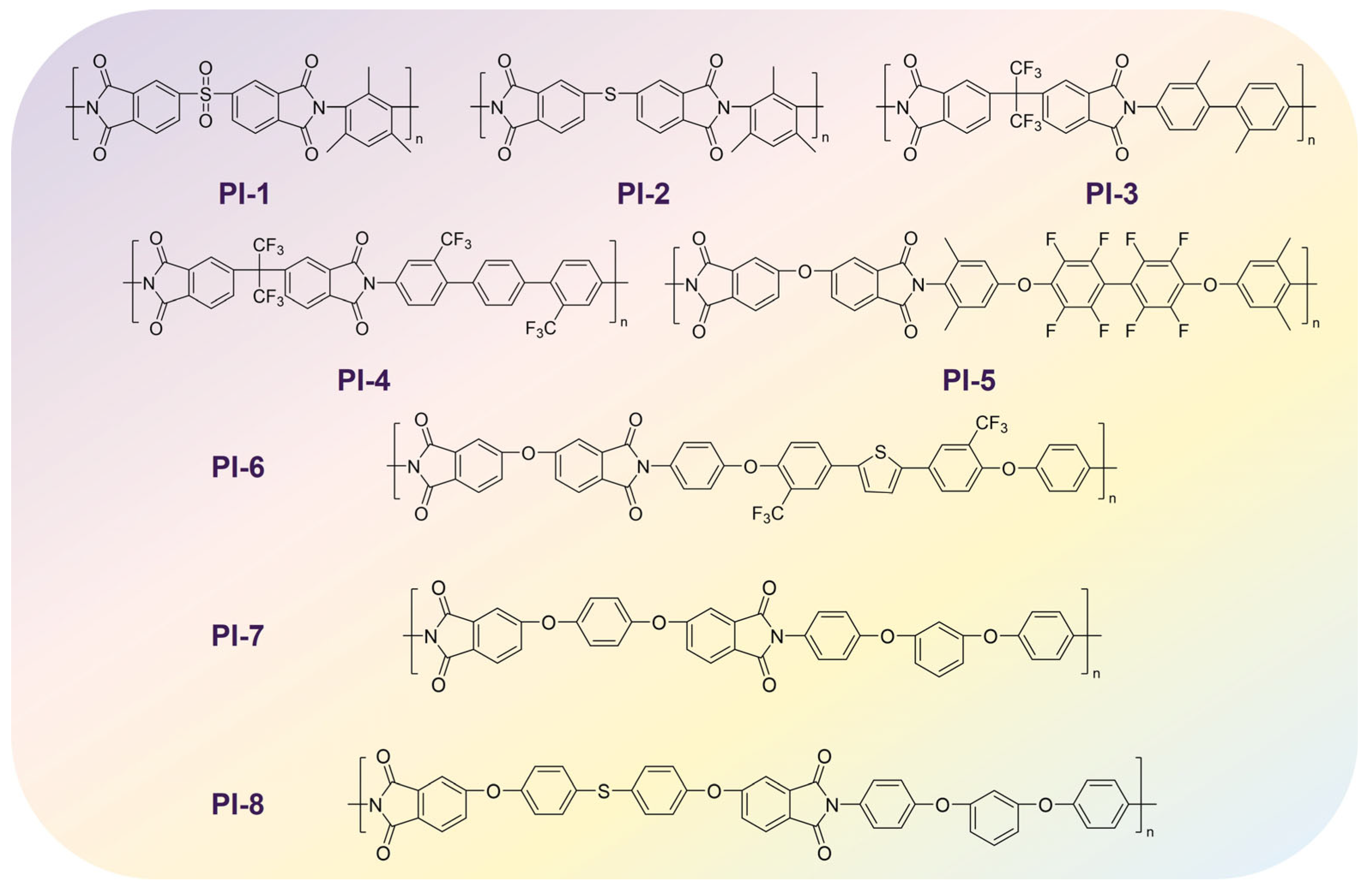
| Name | NumRotatableBonds | ML (°C) | MD (°C) | Experiment (°C) | Diff (%) | Ref. |
|---|---|---|---|---|---|---|
| PI-1 | 3 | 378 | 444 | 418 | 14.87 | [61] |
| PI-2 | 3 | 373 | 400 | 378 | 6.75 | [61] |
| PI-3 | 4 | 345 | 384 | 363.5 | 10.16 | [62] |
| PI-4 | 5 | 308 | 341 | 319 | 9.68 | [63] |
| PI-5 | 8 | 285 | 334 | 302 | 14.67 | [64] |
| PI-6 | 9 | 227 | 246 | 234 | 7.72 | [65] |
| PI-7 | 9 | 196 | 212 | 199 | 7.55 | [66] |
| PI-8 | 11 | 187 | 205 | 178 | 8.78 | [67] |
Disclaimer/Publisher’s Note: The statements, opinions and data contained in all publications are solely those of the individual author(s) and contributor(s) and not of MDPI and/or the editor(s). MDPI and/or the editor(s) disclaim responsibility for any injury to people or property resulting from any ideas, methods, instructions or products referred to in the content. |
© 2025 by the authors. Licensee MDPI, Basel, Switzerland. This article is an open access article distributed under the terms and conditions of the Creative Commons Attribution (CC BY) license (https://creativecommons.org/licenses/by/4.0/).
Share and Cite
Huo, W.; Liang, B.; Wu, X.; Zhang, Z.; Zhou, W.; Wang, H.; Ran, X.; Bai, Y.; Zheng, R. Prediction and Interpretability Study of the Glass Transition Temperature of Polyimide Based on Machine Learning and Molecular Dynamics Simulations. Polymers 2025, 17, 2083. https://doi.org/10.3390/polym17152083
Huo W, Liang B, Wu X, Zhang Z, Zhou W, Wang H, Ran X, Bai Y, Zheng R. Prediction and Interpretability Study of the Glass Transition Temperature of Polyimide Based on Machine Learning and Molecular Dynamics Simulations. Polymers. 2025; 17(15):2083. https://doi.org/10.3390/polym17152083
Chicago/Turabian StyleHuo, Wenjia, Boyang Liang, Xiang Wu, Zhenchang Zhang, Weichao Zhou, Haihong Wang, Xupeng Ran, Yaoyao Bai, and Rongrong Zheng. 2025. "Prediction and Interpretability Study of the Glass Transition Temperature of Polyimide Based on Machine Learning and Molecular Dynamics Simulations" Polymers 17, no. 15: 2083. https://doi.org/10.3390/polym17152083
APA StyleHuo, W., Liang, B., Wu, X., Zhang, Z., Zhou, W., Wang, H., Ran, X., Bai, Y., & Zheng, R. (2025). Prediction and Interpretability Study of the Glass Transition Temperature of Polyimide Based on Machine Learning and Molecular Dynamics Simulations. Polymers, 17(15), 2083. https://doi.org/10.3390/polym17152083