Abstract
Low-dielectric polyimides (PIs) have emerged as essential materials for next-generation microelectronics and communication technologies, yet traditional experimental and theoretical calculation methods for acquiring dielectric constant data face challenges in cost, accuracy, and scalability. This study presents a machine learning (ML) framework that combines polymer domain knowledge with advanced data-driven modeling techniques for accurate prediction of PI dielectric constants at 1 kHz. A dataset of 439 PIs was constructed, and 208 molecular descriptors were derived from SMILES-encoded structures. Through rigorous feature engineering—variance filtering, correlation analysis, and recursive feature elimination—10 key descriptors were identified, capturing electronic and polar interaction, surface area, and structural complexity. Five ML algorithms were evaluated, with Gaussian Process Regression (GPR) achieving superior predictive accuracy (test set: R2 = 0.90, RMSE = 0.10). Shapley additive explanations (SHAP) analysis quantifies the contribution of molecular descriptors to PI dielectric constants. By means of SHAP values, it discloses the positive or negative impacts of descriptors on the predictions. Three novel PIs were synthesized for experimental validation, showing strong agreement between predicted and measured dielectric constants (mean percentage deviation: 2.24%). The model demonstrates robust predictions for other structurally similar polymers but reveals a 40% accuracy reduction (R2 = 0.60) in 10 GHz cross-frequency predictions, emphasizing the requirement for multi-frequency training datasets to enhance model generalizability. This work advances the research paradigm of polymer dielectric materials and provides a pathway for the rational design of materials guided by machine learning.
1. Introduction
Engineering plastics low-dielectric materials are crucial for reducing signal delay, minimizing cross talk, and improving the performance of high-frequency electronics [1,2,3]. Among high-performance polymers, polyimides (PIs) are particularly notable for their exceptional thermal stability, mechanical strength, and chemical resistance. However, conventional PIs often exhibit high dielectric constants, limiting their applications in advanced electronics. This limitation has driven substantial research efforts toward developing low-dielectric-constant alternatives, establishing it as a key objective in contemporary materials science and engineering [4].
Experimental measurements are the primary approach for determining the dielectric constants of PIs; these methods are often time-intensive, expensive, and prone to variability due to inconsistencies in experimental conditions and sample preparation [5,6]. Current computational approaches for dielectric constant prediction, notably quantum chemical calculations and molecular dynamics (MD) simulations [7,8,9], still face distinct challenges. Methods like Density Functional Perturbation Theory (DFPT) are restricted to small systems (<50 atoms) to maintain computational feasibility, and even then neglect dipolar contributions critical for polymer dielectrics [10]. In contrast, classical force fields and MD simulations are computationally efficient but often sacrifice reliability and quantitative accuracy. This discrepancy between computational predictions and experimental results underscores the limitations of relying exclusively on simulation data [11].
Artificial intelligence (AI)-based methods have significantly advanced materials development, enabling predictions of thermal stability [12,13,14], mechanical strength [15,16], and optical transparency [17,18]. Machine learning (ML) has emerged as a powerful tool for utilizing large datasets to predict polymer dielectric properties. However, challenges remain in applying ML to low-dielectric materials, particularly in model interpretability, data quality, and the integration of domain-specific knowledge [19,20].
To alleviate these concerns, a ML framework was developed to predict the dielectric constant of PIs. This methodology combines data science with chemical insights through dataset construction, key molecular descriptor selection, and advanced machine learning algorithms to establish structure–dielectric relationships. The model successfully predicted dielectric constants for three novel PI structures at 1 kHz, demonstrating excellent agreement with experimental values. Furthermore, machine learning models exhibit limited accuracy in predicting the dielectric constant across different frequencies for PIs, with an R2 of 0.60, emphasizing the need for data augmentation at various frequencies. High structural similarity, indicated by a Tanimoto similarity score greater than 0.15, improves prediction accuracy for other polymers.
Figure 1 outlines the workflow for the machine learning-guided dielectric constant prediction of polymer materials. The dataset includes 439 PIs with dielectric constant values reported in the literature at 1 kHz. Initially, the chemical structures of the PIs were converted into SMILES format, and 208 descriptors were extracted using the RDKit package in Python 3.9. Through variance filtering, correlation analysis, and feature importance evaluation, 10 descriptors were identified as representations of structural information. The selected 10 descriptors served as input parameters for training machine learning models using five algorithms: extreme gradient boosting (XGBoost), Gaussian process regression (GPR), random forest (RF), artificial neural network (ANN), and support vector machine (SVM). The trained models predicted dielectric constant at 1 kHz for the PI samples in the test set. Subsequent SHAP analysis revealed descriptor–dielectric relationship. Complete computational details are provided in Section 2.
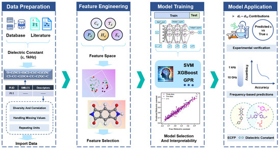
Figure 1.
Machine learning workflow for developing dielectric constant models of PIs, including data preparation, feature engineering, model training and model application.
This study promotes the development of machine learning applied to low dielectric materials, including descriptor selection, model building, and model interpretability. It also clarifies how the structural information of PIs affects dielectric properties, providing theoretical guidance for the design of low dielectric polymers.
2. Methods
Descriptor generation and selection. The PI repeating unit structures were converted to SMILES format, and 208 molecular descriptors were extracted using the RDKit cheminformatics toolkit (see Note S1 for details) [21]. A systematic approach for feature selection was employed. First, variance thresholding was applied [22] with a variance of less than 0.01. From the remaining descriptors, feature importance was assessed using the random forest algorithm. Subsequently, recursive feature elimination (RFE) was utilized to identify the optimal set of descriptors. RFE is an effective feature selection technique that iteratively eliminates the least important features based on model performance until the optimal subset of features is reached [23]. This selection process also considered the correlation of the descriptors with the dielectric constant. Ultimately, some descriptors were finalized for subsequent machine learning modeling. Additionally, due to the frequency dependence of dielectric constants [24], all samples in the dataset were measured at 1 kHz, leading to the exclusion of frequency as a descriptor to maintain data consistency.
Machine learning strategy. Five machine learning algorithms (Figure 2a–e) were evaluated for dielectric constant prediction in PIs, representing diverse modeling approaches: ensemble methods (RF and XGBoost) [25], kernel-based learning (SVM) [26], probabilistic modeling (GPR), and deep learning (ANN) [27]. Since regression algorithms can exhibit varying predictive performances on the same dataset, comparing multiple algorithms helps identify the most accurate and robust model. Model training was implemented using the Scikit-learn library [28], the dataset was split into 80% for training and 20% for testing. Model performance was assessed using R-Square (R2), Root Mean Squared Error (RMSE), and Mean Absolute Error (MAE) by averaging the statistical runs of 30 random training and test splits.
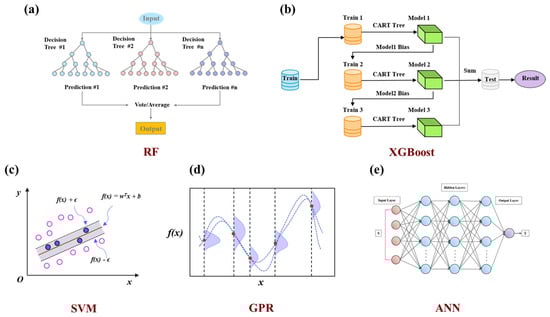
Figure 2.
Comparison of machine learning algorithms for predicting PI dielectric constant: (a) RF. (b) XGBoost. (c) SVM. (d) GPR. (e) ANN.
Evaluation of structural similarity. Structural similarity analysis was conducted to assess model transferability to other polymers. PMDA-ODA, a representative PI structure, and 12 additional polymers were represented by SMILES notation and converted to Extended-Connectivity Fingerprints (ECFPs) [29]. Tanimoto similarity scores between PMDA-ODA and the 12 polymers were calculated to quantify their structural relationships (see Note S2 for calculation details). The Tanimoto similarity score [30] is defined as Equation (1):
The Tanimoto similarity score measures the similarity between two molecular fingerprint vectors, Ps and Pt, where Psk and Ptk represent the k-th components of the fingerprints for molecules s and t, respectively. The numerator calculates the shared features between s and t. The denominator represents the combined features without double-counting shared features. The resulting coefficient ranges from 0 to 1, where 1 indicates identical fingerprints, and 0 indicates no shared features.
Descriptor correlation analysis. Model training was the Pearson correlation coefficient r, which quantifies the strength and direction of a linear relationship between two variables, calculated as Equation (2)
where x and y are one-dimensional arrays of the same length, xi and yi represent individual values within these arrays, and and are the respective sample means. The coefficient r ranges from −1 to 1, with values closer to ±1 indicating a stronger linear relationship and values near 0 indicating little or no linear association.
3. Results and Discussion
Dataset and polymer descriptors. The dataset was compiled from previously published literature (with URLs listed in Table S1). The dielectric constants span from 2.52 to 3.96, with a mean (μ) of 3.09 and a standard deviation (σ) of 0.36 (Figure 3a). Although the distribution is approximately normal, it exhibits slight skewness. To ensure consistency in model inputs, data normalization was applied during the machine learning workflow. Following variance screening, 68 descriptors with a fluctuation variance below 0.01 were removed. Among the remaining 140 descriptors, four pairs were identified with identical values: MaxEStateIndex and MaxAbsEStateIndex, NumAromaticCarbocycles and fr_benzene, fr_Ar_NH and fr_Nhpyrrole, and fr_C_O and fr_C_O_noCOO. To reduce redundancy, MaxEStateIndex, fr_benzene, fr_Ar_NH, and fr_C_O were excluded, as the remaining descriptors offered clearer, more distinct chemical insights.
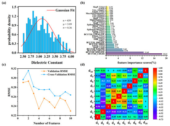
Figure 3.
The dielectric constant values and selected descriptors of PIs. (a) Dielectric constant data distribution, where n is the data sample size, μ is the mean value, and σ is the standard deviation. (b) The feature importance scores of descriptors derived from the random forest algorithm, highlighting the top 30 descriptors. (c) RMSE trends across validation and cross-validation during recursive feature elimination. (d) Correlation coefficients between the top 10 descriptors.
Feature importance scores for descriptors were calculated (Table S2). Figure 3b presents descriptors with feature importance scores of 0.75% or higher, spanning categories such as molecular electrostatic, topological, and molecular surface area descriptors. RFE was utilized to determine the optimal feature subset size. As illustrated in Figure 3c, the validation and cross-validation RMSE values reach their minima at 10 features, representing an optimal trade-off between model accuracy and complexity. The 10 descriptors were selected based on their importance scores and diversity in type, with correlation analysis confirming their independence. The heat map (Figure 3d) demonstrates low-to-moderate pairwise correlations, indicating minimal descriptor redundancy. The final 10 descriptors (Table 1) form an optimized feature set that effectively captures essential chemical information for accurate PI property prediction.

Table 1.
The ten selected descriptors and their definitions.
Effect of selected descriptors on dielectric constant. Ten key descriptors were identified. Descriptors MinEStateIndex (d1), BCUT12D_CHGHI (d3), Chi2n (d4), TPSA (d8), and VSA_EState3 (d10) collectively characterize electronic and polar interaction that influence dielectric behavior. MinEStateIndex (d1) identifies low electronic state atoms in polar groups, particularly electronegative elements (O, N), which enhance molecular polarity and polarizability under alternating electric fields [31]. BCUT2D_CHGHI (d3) measures localized charge density, where high charge concentration regions typically reduce polarizability, showing an inverse relationship with the dielectric constant. Chi2n (d4) reflects the degree of charge separation and local polarity distribution within a molecule. A higher Chi2n (d4) value indicates the presence of a greater number of second-order adjacent atom pairs exhibiting significant charge disparities, which may result in strongly polar regions within the molecular structure. TPSA (d8) measures the total polar surface area, which highlights electronegative regions (Figure 4a) that enhance electric field response [32]. VSA_EState3 (d10) represents the summation of electrotopological state (E-state) indices for atoms whose van der Waals surface area (VSA) values fall within the range of 5.00–5.41 Å2. This descriptor quantifies the electron-surface coupling effects in weakly polar regions of the molecule. Both descriptors (VSA_EState3 (d10) and MinEStateIndex (d1)) are intrinsically linked to the E-State Index framework, as they quantify the electronic characteristics of atoms within a molecule. Therefore, the visualization strategy for VSA_EState3 (d10) can adopt methodologies analogous to those used for MinEStateIndex (d1).
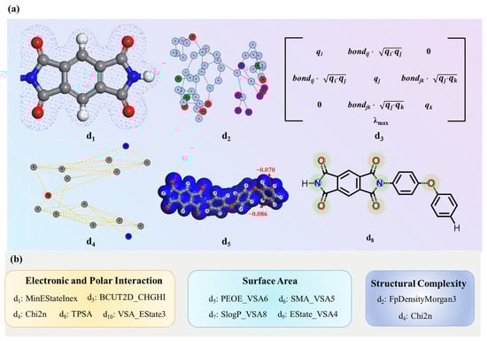
Figure 4.
(a) The chemical significance of selected descriptors. (b) Classification of the ten molecular descriptors.
FpDensityMorgan3 (d2) and Chi2n (d4) characterize structural complexity [33]; a higher FpDensityMorgan3 (d2) value often indicates increased structural complexity due to a greater presence of aromatic or heterocyclic rings and branching [34,35]. Chi2n (d4) quantifies molecular connectivity, where higher values indicate increased branching.
Descriptors PEOE_VSA6 (d5), SMR_VSA5 (d6), SlogP_VSA8 (d7), and EState_VSA4 (d9) assess molecular surface area. As shown in Figure 4a, the blue region represents the VSA values across all atoms in the molecule; PEOE_VSA6 (d5) calculates the VSA values of all atoms whose partial lie between −0.10 and −0.05. SMR_VSA5 (d6) identifies electron-dense regions that hinder charge redistribution and polarization response. SMR_VSA5 (d6), SlogP_VSA8 (d7), and EState_VSA4 (d9) quantify the summation of VSA values for atoms within specific ranges of molar refractivity (SMR), octanol–water partition coefficient (logP), and E-state indices, respectively. While these descriptors are fundamentally tied to VSA contributions, their visualization is omitted from Figure 4a to avoid redundancy, as their graphical representation would follow analogous methodologies to the VSA_EState3 (d10) and MinEStateIndex (d1) mappings already illustrated. Calculation methods of some descriptors are detailed in Table S3. These descriptors comprehensively characterize how electronic and polar interaction, structural complexity, and surface area govern PI dielectric performance (Figure 4b).
Performance Evaluation of ML Models. Five machine learning algorithms were utilized (Figure 5a–e) to build models based on the ten selected descriptors. Model performance was evaluated by comparing experimental and predicted dielectric constants (Table S4). The GPR model exhibited superior predictive accuracy, achieving the lowest RMSE values (0.07 for training, 0.10 for test) and highest R2 values (0.96 for training, 0.90 for test), and demonstrating excellent generalization across the data distribution. These results highlight GPR’s effectiveness in modeling the nonlinear dielectric behavior of PIs, establishing it as an optimal approach for high-precision property prediction. The ANN model demonstrated robust performance, achieving R2 values of 0.90 (training) and 0.85 (test), with corresponding RMSE values of 0.11 and 0.14. Its neural network architecture enables effective capture of complex nonlinear patterns, making it particularly suitable for modeling intricate dependencies in PI dielectric properties. While ANN proves to be a viable approach for handling sophisticated nonlinearities, its predictive accuracy on the test set was marginally lower compared to GPR. The XGBoost and RF models demonstrated moderate predictive performance, each with distinct strengths. XGBoost, utilizing gradient boosting to iteratively correct errors, achieved an R2 of 0.97 for the training set and 0.84 for the test set, with RMSE values of 0.10 and 0.15, respectively. Although the model exhibits high training accuracy, indicating strong data fitting, its relatively lower test performance suggests limited generalization to unseen data. The RF model, a bagging ensemble method, achieved an R2 of 0.89 on the training set and 0.83 on the test set, with RMSE values of 0.11 and 0.15. This performance implies that RF captured certain structural features related to dielectric behavior, but it may lack the precision required to fully represent complex molecular interactions, especially considering the diversity within the dataset. Although the SVM model demonstrated reasonable accuracy, its performance was inferior to that of GPR and ANN, achieving R2 values of 0.87 (training) and 0.82 (test), with RMSE values of 0.13 and 0.16, respectively. This lower performance likely reflects the sensitivity of SVM to complex data distributions and susceptibility to noise in the dataset.
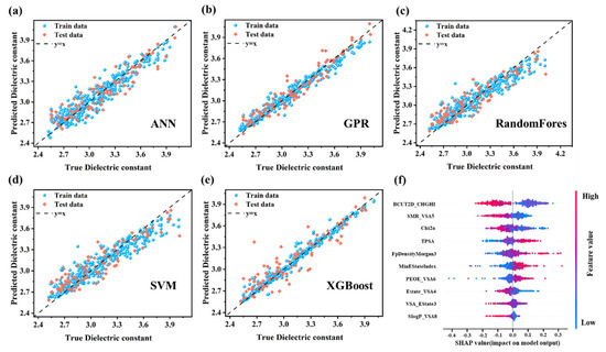
Figure 5.
Performance evaluation of machine learning regression models for PI dielectric constant prediction: (a) ANN, (b) GPR, (c) RF, (d) SVM, and (e) XGBoost. (f) SHAP value distribution of selected descriptors.
While machine learning models demonstrate strong predictive accuracy for PI dielectric constants, their practical applicability and reliability heavily depend on model interpretability [36]. To address this critical aspect, we implemented the XGBoost algorithm coupled with Shapley additive explanations (SHAP), a game theory-based approach that quantifies individual feature contributions to model predictions [37]. The integration is superior to other models, including TreeExplainer’s deterministic Shapley value calculation, high computational efficiency, and hierarchical feature interaction mapping [38,39]. Figure 5f illustrates two key aspects of the model’s dielectric constant predictions: (1) the critical molecular descriptors influencing the predictions and (2) their directional impacts on the results (positive or negative). Descriptors are ranked vertically in descending order of importance, where BCUT2D_CHGHI exhibits the strongest predictive influence, followed by SMR_VSA5, while SlogP_VSA8 contributes minimally. Each data point represents a sample’s descriptor value, with red and blue colors corresponding to higher and lower descriptor magnitudes, respectively. The horizontal SHAP value axis quantifies directional effects: positive SHAP values (rightward points) increase dielectric constant prediction values, whereas negative values (leftward points) decrease the predictions. Taking TPSA as an example, the majority of red points cluster in the positive SHAP region, while blue points dominate the negative zone. This indicates higher TPSA values correlate with increased dielectric constant predictions, whereas lower TPSA values reduce predictions. Such behavior aligns with the fundamental relationship between molecular polar surface area and dielectric properties, reinforcing the physicochemical interpretability of the model.
Figure 6, generated via Python code, presents a Force Plot that visually compares the impacts of descriptors on dielectric constant predictions for two distinct samples. The base value (3.09), derived as the mean of 439 collected PI samples, serves as the model’s initial reference point. The f(x) values denote the actual predicted dielectric constants for individual samples. These predictions are calculated relative to the baseline, with descriptors enhancing the dielectric constant highlighted in red and those reducing it in blue. The numerical annotations adjacent to each descriptor indicate their specific molecular values. For sample 1 (predicted value: 2.95), the descriptors predominantly responsible for reducing the dielectric constant, such as BCUT2D_CHGHI, TPSA, MinEStateIndex, and PEOE_VSA6, exhibit a synergistic interaction, collectively driving the prediction below the baseline.
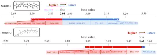
Figure 6.
Descriptor impact analysis on dielectric constant prediction for two representative PI structures.
Notably, while the descriptors like SMR_VSA5, SlogP_VSA8, VSA_Estate3, and Chi2n partially counterbalance this trend by increasing the dielectric constant, their contributions remain insufficient to reverse the overall downward prediction. For the other two descriptors, EState_VSA4 and FpDensityMorgan3, the contribution to the dielectric constant prediction for this sample is small. In contrast, sample 2, with predicted value of 3.62, demonstrates a significant elevation above the base value, driven by seven dominant descriptors that amplify the dielectric constant: TPSA, BCUT2D_CHGHI, Chi2n, SMR_VSA5, Estate_VSA4, MinEStateIndex, and SlogP_VSA8. Of particular interest is the dual regulatory behavior of BCUT2D_CHGHI: while suppressing dielectric constant in sample 1, it enhances the prediction in sample 2. This reversal highlights the strong dependence of descriptors on molecular bonding configurations and its mechanistic link to spatial reorientation of molecular dipoles. This interpretability framework not only validates the role of TPSA in classical dielectric theory but also uncovers critical contributions from counterintuitive descriptors such as Chi2n and BCUT2D_CHGHI. These findings establish a robust descriptor foundation for the rational multiscale design of dielectric materials. By strategically leveraging descriptor synergies, this approach holds promise for overcoming the limitations of empirical trial-and-error methodologies.
Experimental validation and extension of the dielectrics constant prediction model. Based on monomer synthesis feasibility, membrane preparation practicality, and chemical structure representativeness, three PIs—PI-a, PI-b, and PI-c—were selected as optimal candidates for experimental validation (Figure 7a). These PIs were successfully synthesized (Note S3 for experimental details) and their dielectric constants were determined, as shown in Figure 7b. At 1 kHz, PI-a demonstrated the highest dielectric constant (4.11), whereas PI-c exhibited the lowest (2.99). The GPR model was utilized to predict dielectric constants of the three PIs to further validate its predictive capability, yielding values of 4.01 (PI-a), 3.30 (PI-b), and 2.88 (PI-c) at 1 kHz (Figure 7c). The GPR model-predicted dielectric constants showed a slight underestimation compared to the experimental values, with an average percentage deviation of 2.24% (Table S5). Notably, both values exhibited consistent trends within acceptable experimental error margins.
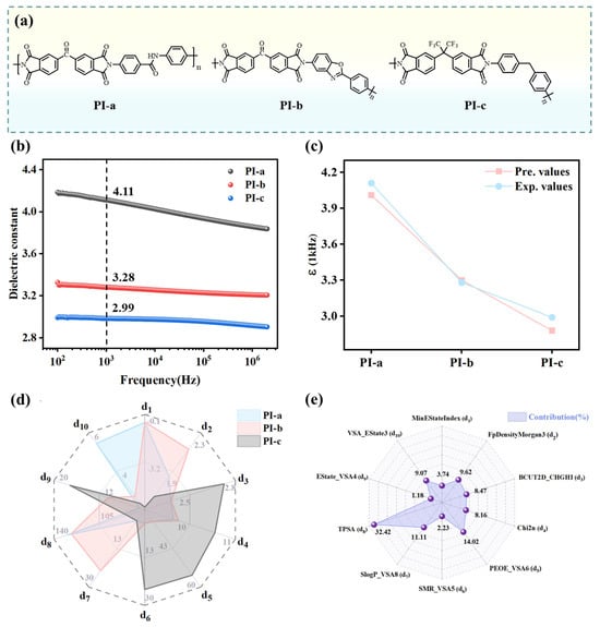
Figure 7.
(a) Structures of the three PIs. (b) Frequency-dependent dielectric constants of PIs. (c) Comparison between experimental and predicted dielectric constants. (d) Calculated descriptor values for PI-a, PI-b, and PI-c. (e) Calculated ten descriptor contributions.
The differences in dielectric constants of the three PIs can be explained from the perspectives of both molecular structures and the descriptors. Structurally, PI-a and PI-b incorporate polar functional groups (e.g., carbonyl) with broader polar region distributions, leading to larger dipole moments. This enhances dipolar polarization under an electric field, thereby increasing their dielectric constants. The CF3 groups in PI-c exhibit a strong electron-withdrawing effect, which effectively reduces the polarizability. Furthermore, the incorporation of the sterically bulky CF3 groups disrupts the ordered packing of polymer chains, resulting in increased free volume. This structural modification synergistically contributes to lowering the dielectric constant.
Moreover, ten descriptors were evaluated for their contributions to the three PIs using sensitivity analysis (Table S6). This involved systematically perturbing each descriptor value while monitoring corresponding shifts in GPR model predictions to establish parameter influence. As shown in Figure 7d, PI-a and PI-b demonstrate significantly higher TPSA (d8) values than PI-c, reflecting their broader distribution of polar regions, a critical factor for enhanced dielectric properties. This observation is further supported by the descriptor contribution analysis (Figure 7e), where TPSA (d8) exhibits the highest contribution (32.42%). The MinEStateIndex (d1) values for PI-a and PI-b were calculated at −0.61 and −0.57, respectively, while PI-c exhibited a MinEStateIndex of −6.03. A smaller (more negative) MinEStateIndex value indicates the presence of stronger electron-withdrawing groups within the molecular structure. This substantial reduction in PI-c arises from the strong electron-withdrawing CF3 group, which induces extreme electron deficiency at specific carbon atoms. The pronounced electronegativity of fluorine atoms localized electron density in discrete molecular regions, creating an uneven dipole moment distribution, thereby resulting in a lower dielectric constant. The Estate_VSA4 (d9) demonstrated minimal contribution (1.18%), which quantifies the surface area contributions of atoms within an E-state index range (1.17–1.54), corresponding to regions of moderate polarity. The prevalence of atomic environments likely facilitated dielectric constant reduction by limiting excessive charge separation.
Descriptors BCUT2D_CHGHI (d3) and Chi2n (d4) quantify the balance between molecular topological complexity and local charge distribution. For PI-a and PI-b, BCUT2D_CHGHI (d3) and Chi2n (d4) values indicate a compromise between structural sophistication and charge delocalization. This balanced molecular architecture mitigates dynamic response constraints while maintaining sufficient polarization flexibility under external electric fields. PI-c demonstrates excessive charge localization and elevated topological complexity, constraining polarization pathways and diminishing dielectric response. SMR_VSA5 (d6) quantifies surface area distribution based on molar refractivity and correlates with molecular volume, revealing critical structural distinctions. The SMR_VSA5 value for PI-c is notably high, reaching 24.19. This is due to the presence of bulky -CF3 groups, which restrict the mobility of molecular chain segments and increase spatial hindrance. As a result, its dielectric constant is reduced. FpDensityMorgan3 (d2) reflects functional group density derived from Morgan fingerprints. PI-b exhibits a higher FpDensityMorgan3 value (2.13) compared to PI-a (1.85), suggesting the incorporation of additional functional groups. However, its dielectric constant lines between that of PI-a and PI-c due to the absence of steric-restrictive groups and high polar surface area contributions. For PI-c, the low FpDensityMorgan3 (d2) value (1.64) highlights a trade-off: the introduction of -CF3 substituents diminishes the density of other polar functional groups. This reduction partially counteracts the high polarization implied by its elevated PEOE_VSA6 value (54.59), ultimately limiting dielectric enhancement.
Based on descriptor contributions, to design PIs with lower dielectric constants, two main strategies could be adopted. First, reducing the TPSA helps to control the spatial distribution of polar groups. Second, introducing bulky groups, such as trifluoromethyl and adamantly, serves multiple purposes. These groups can increase the molecular volume, regulate the molar refractive index surface area (SMR_VSA5 (d6)), and restrict the movement of molecular segments through steric hindrance. This, in turn, can suppress the ability of dipole rearrangement. In addition, weak polar groups are concentrated in non-conjugated regions to optimize the density of functional groups (FpDensityMorgan3 (d2)). Finally, it is necessary to balance the post-molecular topological complexity and local charge distribution, which can limit the polarization path and reduce the dielectric response.
This study further demonstrates the expanded applicability of machine learning models in predicting frequency-dependent dielectric properties of polymers. It also evaluates their generalizability across diverse polymeric systems. As illustrated in Figure 8a, the GPR model shows limited predictive capability (R2 = 0.60, MAE = 0.17, RMSE = 0.22) for 36 PIs at 10 GHz [40], highlighting the challenges in cross-frequency extrapolation. This performance constraint stems from the model’s inability to capture complex polarization dynamics [24], including electronic, atomic, and orientational effect. These dynamics govern dielectric responses across broad frequency spectra. Future studies should focus on developing multi-frequency training datasets to better capture the spectrum of polarization mechanisms.
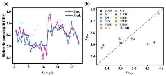
Figure 8.
The application of machine learning models in distinct scenarios: (a) dielectric constant prediction of polyimide at 10 GHz, and (b) comparative dielectric constant prediction of various polymer materials at 1 kHz.
The model’s generalizability across polymer systems was systematically evaluated, as shown in Figure 8b. The GPR model demonstrated high predictive accuracy for PEEU, PC, PPS, and POFNB, but showed significant deviations for BOPP, PTFE, and PU. This highlights material-specific performance variations among the 12 polymers (structural details in Figure S1) [41,42]. Tanimoto similarity analysis between target polymers and PMDA-ODA (Table 2) revealed a correlation between structural similarity and prediction accuracy (e.g., PEEU = 0.32, PC = 0.15, PPS = 0.16). This indicates the model’s ability to capture essential PI structure features through domain-informed feature engineering. Based on these findings, optimizing PI-ML models should prioritize data augmentation using polymers with high structural similarity (Tanimoto similarity score > 0.15) or comparable polarity. For structurally dissimilar systems like BOPP and PTFE, cautious inclusion is recommended.
Table 2.
Similarity comparison of polyimide with various polymers based on Tanimoto similarity scores.
4. Conclusions
This work establishes a machine learning framework for accurately predicting polyimide dielectric constants, adding a new path for dielectric polymer material discovery. By integrating feature engineering and interpretable ML, the GPR model identified structural descriptors governing dielectric behavior, validated through experimental synthesis. The model’s high accuracy and interpretability underscore its utility in guiding PI design, particularly for reducing polar surface areas and optimizing charge distribution. However, the limited generalizability to dissimilar polymers and cross-frequency predictions highlights the necessity of augmenting datasets with multi-frequency measurements. Future work should focus on expanding descriptor diversity and incorporating dynamic polarization mechanisms to enhance predictive capabilities across broader material classes and frequency ranges. These insights facilitate the accelerated development of low-dielectric polymers tailored for electronic applications.
Supplementary Materials
The following supporting information can be downloaded at: https://www.mdpi.com/article/10.3390/polym17121622/s1.
Author Contributions
X.H.: Conceptualization, Methodology, Writing—original draft, Formal analysis, Data curation, Software. J.W.: Visualization, Validation, Data curation. S.Z.: Writing—review and editing. C.Z.: Methodology, Validation. P.X.: Methodology, Validation. F.Z.: Writing—review and editing, Supervision. Q.L.: Funding acquisition, Writing—review and editing, Supervision. All authors have read and agreed to the published version of the manuscript.
Funding
This work was financially supported by the National Natural Science Foundation of China (grant nos. 52233016 and 52350337). The authors thank the South African Centre for High-Performance Computing (CHPC) for donating the cluster facility, which was used to perform the computational work.
Institutional Review Board Statement
Not applicable.
Data Availability Statement
Data will be made available on request.
Conflicts of Interest
The authors declare that they have no known competing financial interests or personal relationships that could have appeared to influence the work reported in this paper.
References
- Volksen, W.; Miller, R.D.; Dubois, G. Low Dielectric Constant Materials. Chem. Rev. 2010, 110, 56–110. [Google Scholar] [CrossRef] [PubMed]
- Wang, Z.; Zhang, M.; Han, E.; Niu, H.; Wu, D. Structure-property relationship of low dielectric constant polyimide fibers containing fluorine groups. Polymer 2020, 206, 122884. [Google Scholar] [CrossRef]
- He, X.; Zhang, S.; Zhou, Y.; Zheng, F.; Lu, Q. The “fluorine impact” on dielectric constant of polyimides: A molecular simulation study. Polymer 2022, 254, 125073. [Google Scholar] [CrossRef]
- Bei, R.; Qian, C.; Zhang, Y.; Chi, Z.; Liu, S.; Chen, X.; Xu, J.; Aldred, M.P. Intrinsic low dielectric constant polyimides: Relationship between molecular structure and dielectric properties. J. Mater. Chem. C 2017, 5, 12807–12815. [Google Scholar] [CrossRef]
- Chen, J.; Pei, Z.; Chai, B.; Jiang, P.; Ma, L.; Zhu, L.; Huang, X. Engineering the Dielectric Constants of Polymers: From Molecular to Mesoscopic Scales. Adv. Mater. 2024, 36, 2308670. [Google Scholar] [CrossRef]
- Li, J.; Cai, J.; Yu, J.; Li, Z.; Ding, B. The Rising of Fiber Constructed Piezo/Triboelectric Nanogenerators: From Material Selections, Fabrication Techniques to Emerging Applications. Adv. Funct. Mater. 2023, 33, 2303249. [Google Scholar] [CrossRef]
- Ma, R.; Baldwin, A.F.; Wang, C.; Offenbach, I.; Cakmak, M.; Ramprasad, R.; Sotzing, G.A. Rationally Designed Polyimides for High-Energy Density Capacitor Applications. ACS Appl. Mater. Interfaces 2014, 6, 10445–10451. [Google Scholar] [CrossRef]
- Chua, J.; Tu, Q. A Molecular Dynamics Study of Crosslinked Phthalonitrile Polymers: The Effect of Crosslink Density on Thermomechanical and Dielectric Properties. Polymers 2018, 10, 64. [Google Scholar] [CrossRef]
- Zhang, D.; Li, Y.; Lu, H.; Zhao, F.; Cheng, J.; Zhang, J. Influence of conversion on dielectric constant of Dicyandiamide cured epoxy resin:a molecular dynamic simulation and experiment study. Polymer 2023, 267, 125645. [Google Scholar] [CrossRef]
- Chen, L.; Kim, C.; Batra, R.; Lightstone, J.P.; Wu, C.; Li, Z.; Deshmukh, A.A.; Wang, Y.; Tran, H.D.; Vashishta, P.; et al. Frequency-dependent dielectric constant prediction of polymers using machine learning. NPJ Comput. Mater. 2020, 6, 61. [Google Scholar] [CrossRef]
- Tran, H.; Gurnani, R.; Kim, C.; Pilania, G.; Kwon, H.-K.; Lively, R.P.; Ramprasad, R. Design of functional and sustainable polymers assisted by artificial intelligence. Nat. Rev. Mater. 2024, 9, 866–886. [Google Scholar] [CrossRef]
- Raccuglia, P.; Elbert, K.C.; Adler, P.D.F.; Falk, C.; Wenny, M.B.; Mollo, A.; Zeller, M.; Friedler, S.A.; Schrier, J.; Norquist, A.J. Machine-learning-assisted materials discovery using failed experiments. Nature 2016, 533, 73–76. [Google Scholar] [CrossRef] [PubMed]
- Zhang, S.; He, X.; Xia, X.; Xiao, P.; Wu, Q.; Zheng, F.; Lu, Q. Machine-Learning-Enabled Framework in Engineering Plastics Discovery: A Case Study of Designing Polyimides with Desired Glass-Transition Temperature. ACS Appl. Mater. Interfaces 2023, 15, 37893–37902. [Google Scholar] [CrossRef] [PubMed]
- Wu, S.; Kondo, Y.; Kakimoto, M.-a.; Yang, B.; Yamada, H.; Kuwajima, I.; Lambard, G.; Hongo, K.; Xu, Y.; Shiomi, J.; et al. Machine-learning-assisted discovery of polymers with high thermal conductivity using a molecular design algorithm. NPJ Comput. Mater. 2019, 5, 66. [Google Scholar] [CrossRef]
- Hu, Y.; Zhao, W.; Wang, L.; Lin, J.; Du, L. Machine-Learning-Assisted Design of Highly Tough Thermosetting Polymers. ACS Appl. Mater. Interfaces 2022, 14, 55004–55016. [Google Scholar] [CrossRef]
- Gao, L.; Lin, J.; Wang, L.; Du, L. Machine Learning-Assisted Design of Advanced Polymeric Materials. Acc. Mater. Res. 2024, 5, 571–584. [Google Scholar] [CrossRef]
- Zhang, Y.; Ling, C. A strategy to apply machine learning to small datasets in materials science. NPJ Comput. Mater. 2018, 4, 25. [Google Scholar] [CrossRef]
- Zhang, S.; He, X.; Xiao, P.; Xia, X.; Zheng, F.; Xiang, S.; Lu, Q. Interpretable Machine Learning for Investigating the Molecular Mechanisms Governing the Transparency of Colorless Transparent Polyimide for OLED Cover Windows. Adv. Funct. Mater. 2024, 34, 2409143. [Google Scholar] [CrossRef]
- Huan, T.D.; Mannodi-Kanakkithodi, A.; Kim, C.; Sharma, V.; Pilania, G.; Ramprasad, R. A polymer dataset for accelerated property prediction and design. Sci. Data 2016, 3, 160012. [Google Scholar] [CrossRef]
- Sharma, V.; Wang, C.; Lorenzini, R.G.; Ma, R.; Zhu, Q.; Sinkovits, D.W.; Pilania, G.; Oganov, A.R.; Kumar, S.; Sotzing, G.A.; et al. Rational design of all organic polymer dielectrics. Nat. Commun. 2014, 5, 4845. [Google Scholar] [CrossRef]
- Duarte Ramos Matos, G.; Pak, S.; Rizzo, R.C. Descriptor-Driven de Novo Design Algorithms for DOCK6 Using RDKit. J. Chem. Inf. Model. 2023, 63, 5803–5822. [Google Scholar] [CrossRef] [PubMed]
- Schiessler, E.J.; Würger, T.; Lamaka, S.V.; Meißner, R.H.; Cyron, C.J.; Zheludkevich, M.L.; Feiler, C.; Aydin, R.C. Predicting the inhibition efficiencies of magnesium dissolution modulators using sparse machine learning models. NPJ Comput. Mater. 2021, 7, 193. [Google Scholar] [CrossRef]
- Kuang, J.; Long, Z. Prediction model for corrosion rate of low-alloy steels under atmospheric conditions using machine learning algorithms. Int. J. Miner. Metall. Mater. 2024, 31, 337–350. [Google Scholar] [CrossRef]
- Sawada, R.; Ando, S. Polarization Analysis and Humidity Dependence of Dielectric Properties of Aromatic and Semialicyclic Polyimides Measured at 10 GHz. J. Phys. Chem. C 2024, 128, 6979–6990. [Google Scholar] [CrossRef]
- Zhang, R.; Li, Y.; Goh, A.T.C.; Zhang, W.; Chen, Z. Analysis of ground surface settlement in anisotropic clays using extreme gradient boosting and random forest regression models. J. Rock Mech. Geotech. Eng. 2021, 13, 1478–1484. [Google Scholar] [CrossRef]
- Zhang, L.; Qian, K.; Huang, J.; Liu, M.; Shibuta, Y. Molecular dynamics simulation and machine learning of mechanical response in non-equiatomic FeCrNiCoMn high-entropy alloy. J. Mater. Res. Technol. 2021, 13, 2043–2054. [Google Scholar] [CrossRef]
- Mohammed, A.S.; Almutahhar, M.; Sattar, K.; Alhajeri, A.; Nazir, A.; Ali, U. Deep learning based porosity prediction for additively manufactured laser powder-bed fusion parts. J. Mater. Res. Technol. 2023, 27, 7330–7335. [Google Scholar] [CrossRef]
- Liu, K.; Wang, F.; Wang, X.; Yan, B.; Tong, M. Prediction of elastic properties of 3D orthogonal woven composites by multiscale deep neural network. Mater. Today Commun. 2025, 42, 111221. [Google Scholar] [CrossRef]
- O’Boyle, N.M.; Sayle, R.A. Comparing structural fingerprints using a literature-based similarity benchmark. J. Cheminform. 2016, 8, 36. [Google Scholar] [CrossRef]
- Rácz, A.; Bajusz, D.; Héberger, K. Life beyond the Tanimoto coefficient: Similarity measures for interaction fingerprints. J. Cheminform. 2018, 10, 48. [Google Scholar] [CrossRef]
- He, Y.; Yang, A.; Zou, C.; Fan, T.; Lan, Q.; He, Y.; Wang, M.; Sunarso, J.; Kong, Z.Y. An interpretable surrogate model for H2S solubility forecasting in ionic liquids based on machine learning. Sep. Purif. Technol. 2025, 357, 130061. [Google Scholar] [CrossRef]
- Chakraborty, N.; Das, S.; Saha, D.; Mondal, S. Surface-analyte interaction as a function of topological polar surface area of analytes in metal (Cd, Al, Ti, Sn) sulfide, nitride and oxide based chemiresistive materials. Sens. Actuators A Phys. 2022, 341, 113610. [Google Scholar] [CrossRef]
- He, X.; Zhang, S.; Zhang, C.; Xiao, P.; Zheng, F.; Lu, Q. Decoding high-frequency dielectric loss of Poly(ester imide)s: Molecular simulation and experiment validation. Polymer 2024, 308, 127337. [Google Scholar] [CrossRef]
- Tian, Y.; Zhang, S.; Yin, H.; Yan, A. Quantitative structure-activity relationship (QSAR) models and their applicability domain analysis on HIV-1 protease inhibitors by machine learning methods. Chemom. Intell. Lab. Syst. 2020, 196, 103888. [Google Scholar] [CrossRef]
- Bo, W.; Qin, D.; Zheng, X.; Wang, Y.; Ding, B.; Li, Y.; Liang, G. Prediction of bitterant and sweetener using structure-taste relationship models based on an artificial neural network. Food Res. Int. 2022, 153, 110974. [Google Scholar] [CrossRef]
- Wang, T.; Hu, J.; Ouyang, R.; Wang, Y.; Huang, Y.; Hu, S.; Li, W.-X. Nature of metal-support interaction for metal catalysts on oxide supports. Science 2024, 386, 915–920. [Google Scholar] [CrossRef]
- Alam, S.M.K.; Li, P.; Rahman, M.; Fida, M.; Elumalai, V. Key factors affecting groundwater nitrate levels in the Yinchuan Region, Northwest China: Research using the eXtreme Gradient Boosting (XGBoost) model with the SHapley Additive exPlanations (SHAP) method. Environ. Pollut. 2025, 364, 125336. [Google Scholar] [CrossRef]
- Zhang, S.; Lei, H.; Zhou, Z.; Wang, G.; Qiu, B. Fatigue life analysis of high-strength bolts based on machine learning method and SHapley Additive exPlanations (SHAP) approach. Structures 2023, 51, 275–287. [Google Scholar] [CrossRef]
- Song, Z.; Cao, S.; Yang, H. An interpretable framework for modeling global solar radiation using tree-based ensemble machine learning and Shapley additive explanations methods. Appl. Energy 2024, 364, 123238. [Google Scholar] [CrossRef]
- Kuo, C.-C.; Lin, Y.-C.; Chen, Y.-C.; Wu, P.-H.; Ando, S.; Ueda, M.; Chen, W.-C. Correlating the Molecular Structure of Polyimides with the Dielectric Constant and Dissipation Factor at a High Frequency of 10 GHz. ACS Appl. Polym. Mater. 2021, 3, 362–371. [Google Scholar] [CrossRef]
- Li, H.; Zhou, Y.; Liu, Y.; Li, L.; Liu, Y.; Wang, Q. Dielectric polymers for high-temperature capacitive energy storage. Chem. Soc. Rev. 2021, 50, 6369–6400. [Google Scholar] [CrossRef]
- Luo, S.; Yu, J.; Ansari, T.Q.; Yu, S.; Xu, P.; Cao, L.; Huang, H.; Sun, R.; Wong, C.-P. Elaborately fabricated polytetrafluoroethylene film exhibiting superior high-temperature energy storage performance. Appl. Mater. Today 2020, 21, 100882. [Google Scholar] [CrossRef]
Disclaimer/Publisher’s Note: The statements, opinions and data contained in all publications are solely those of the individual author(s) and contributor(s) and not of MDPI and/or the editor(s). MDPI and/or the editor(s) disclaim responsibility for any injury to people or property resulting from any ideas, methods, instructions or products referred to in the content. |
© 2025 by the authors. Licensee MDPI, Basel, Switzerland. This article is an open access article distributed under the terms and conditions of the Creative Commons Attribution (CC BY) license (https://creativecommons.org/licenses/by/4.0/).