
Cheminformatics Approaches to the Analysis of Additives for Sustainable Polymeric Materials


Abstract
1. Introduction
2. Materials and Methods
- Install the packages necessary for the analysis and visualization from R 4.2.3. These are chemometrics, ‘ChemmineR’, ‘cluster’, ‘factoextra’, ‘fingerprint’, ‘fmcsR’, ‘ggplot2’, ‘gridExtra’, ‘NbClust’, ‘rcdk’, ‘rgl’, and ‘vegan’.
- Import the compounds in R, in a structure definition file (SDF) format from PubChem [55]. These are in a 2D representation, given that this is one of the most used formats in the study of similarity and neighborhood relationships [42,50]. However, we should mention that there is no best representation, as its appropriateness depends on the study’s goal [42].
- Create the ‘Sdfset’ instance containing all study molecules.
- Visualize the compounds’ IDs and structures using the command ‘view(Sdfset)’.
- 5.
- Plot the compounds’ structure using the command ‘plot(sdfset, …)’.
- 6.
- Detect the molecular descriptors using the ‘propma’ command from ChemmineR.
- 7.
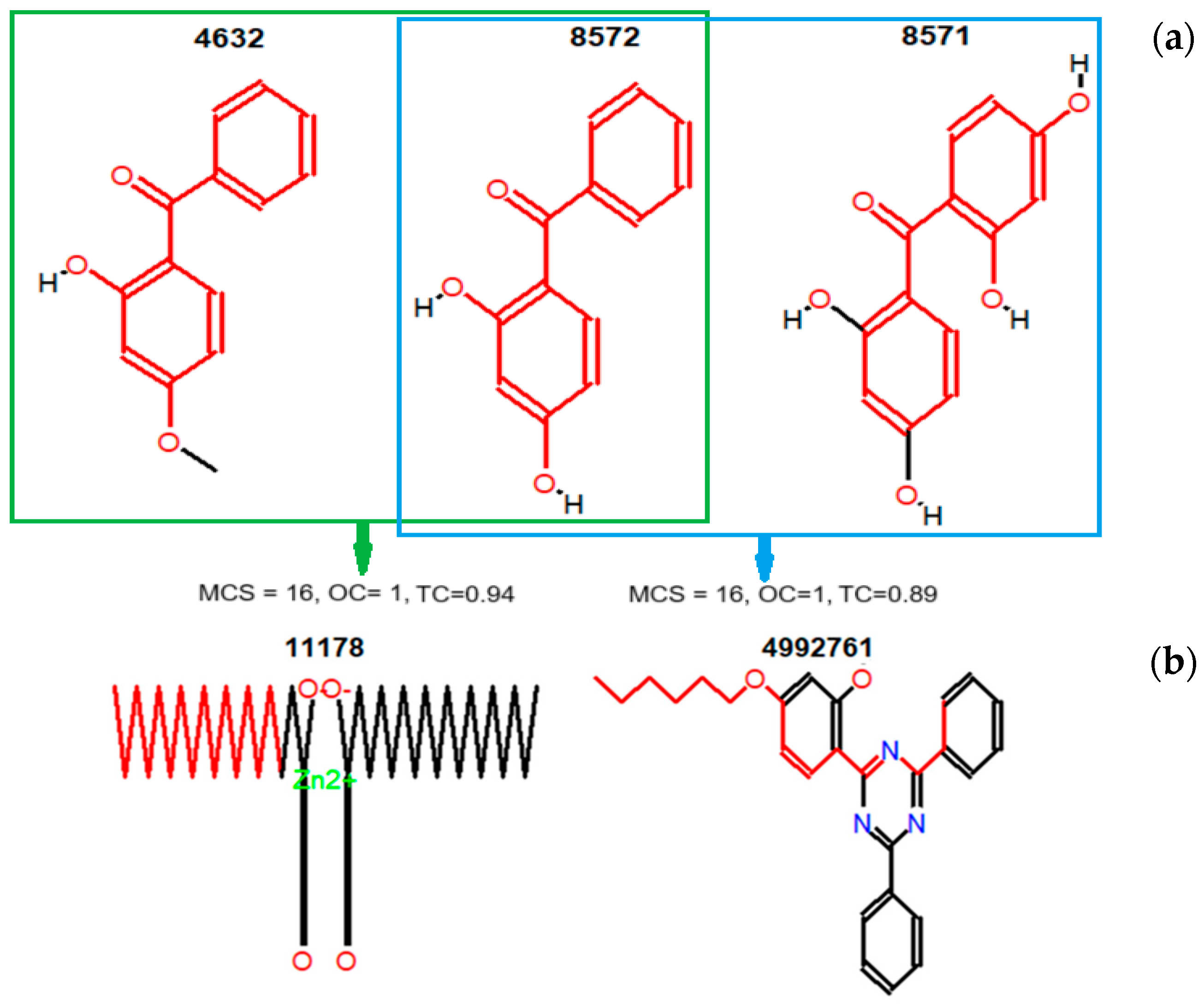
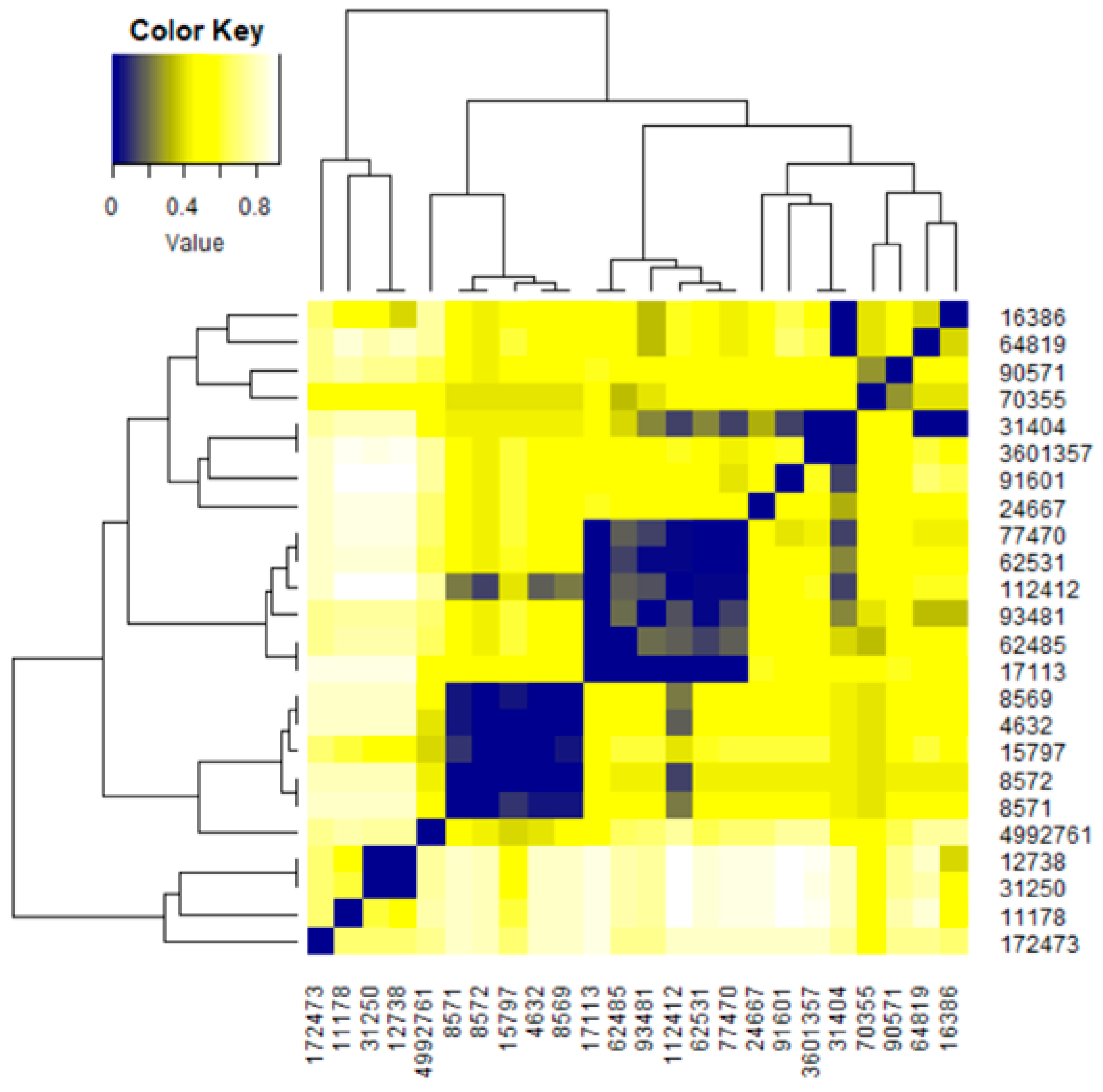
- Evaluate the structures’ similarity using the commands from ChemmineR and ‘fmcsBatch()’ from ‘fmcsR’.
- 8.
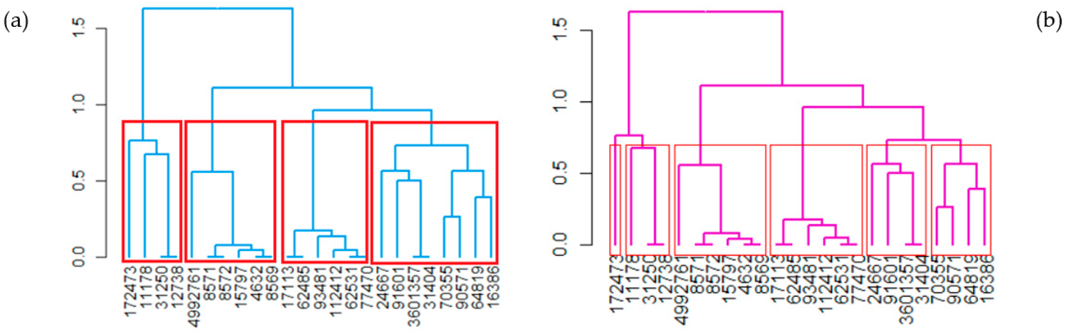
- Cluster the Molecules
- Binning, which is based on the molecules’ characteristics from which a distance matrix is built. During the algorithm run, the clusters are merged using the single linkage method. Moreover, different cutoffs are provided given that the optimum cutoff is unknown [74]. This procedure is implemented in the ‘ChemmineR’ package.
3. Results
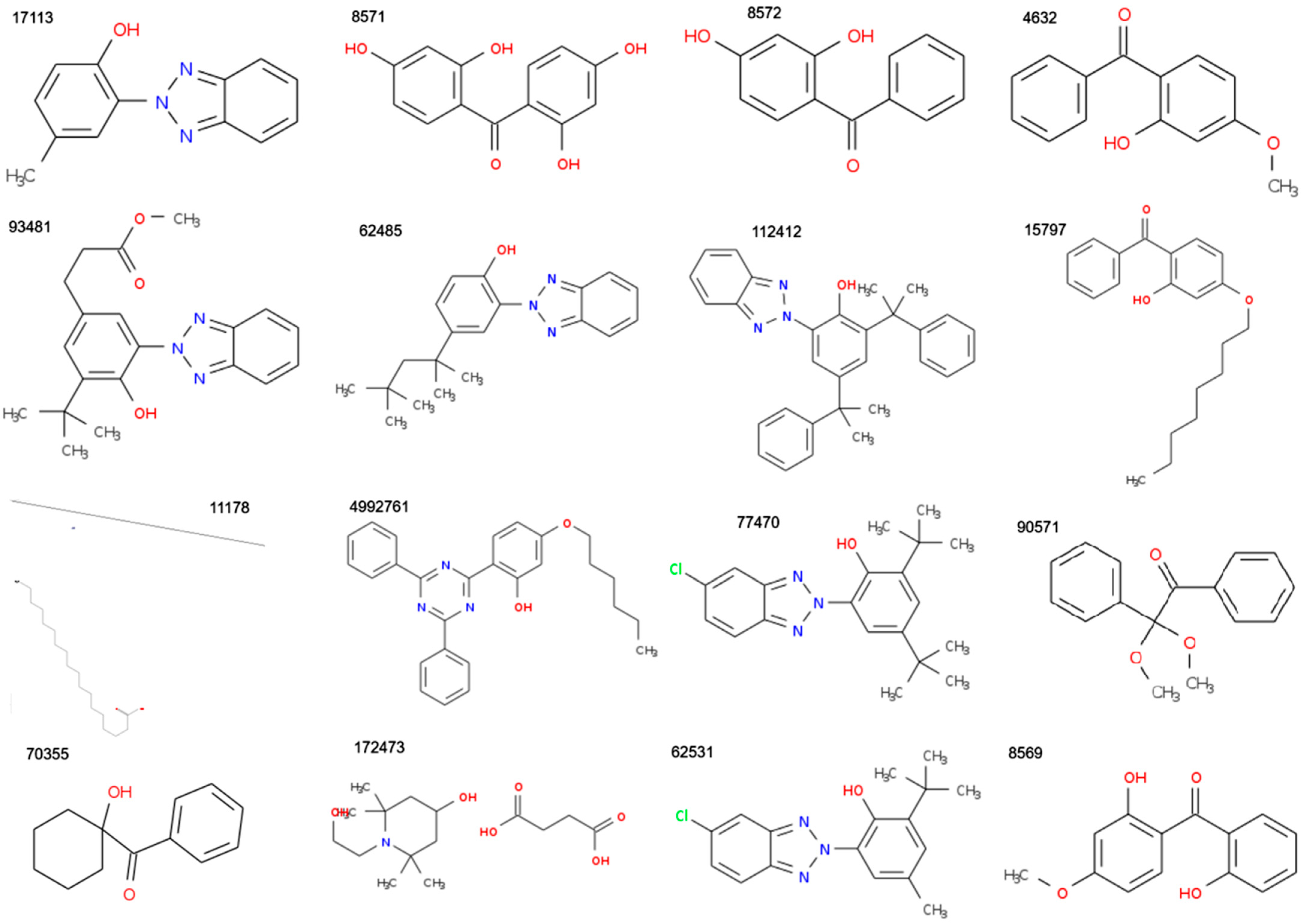
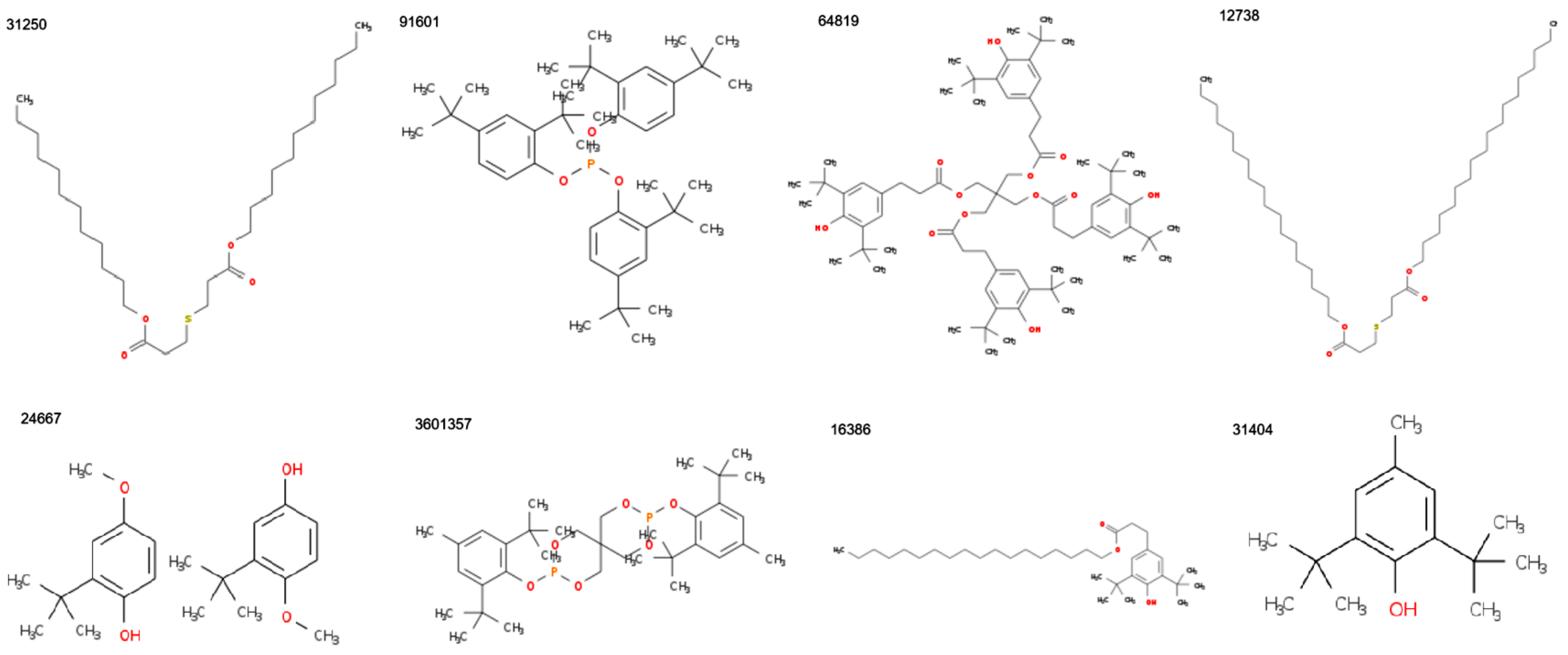
- A quencher—butanedioic acid;1-(2-hydroxyethyl)-2,2,6,6-tetramethylpiperidin-4-ol (HALS GW 622—CID 172473)—CL1.1;
- A heat stabilizer—zinc stearate (CID 11178)—CL1.2;
- Two antioxidants—dodecyl 3-(3-dodecoxy-3-oxopropyl)sulfanylpropanoate (Irganox PS 800—CID 31250) and octadecyl 3-(3-octadecoxy-3-oxopropyl)sulfanylpropanoate (Songnox®DSTDP—CID 12738)—CL1.2.
- Four UV stabilizers, as follows: CID 17113—2-(2′-hydroxy-5′-methylphenyl)-benzophenone; CID 62531—(2′-Hydroxy-3′-tert-5′-methylphenyl)-5-chlorobenzotriazole; CID 77470—2-(2′-hydroxy-3′,5′-di-tert-butylphenyl)-5-chlorobenzotriazole; and CID 112412—2-(2H-Benzotriazol-2-yl)-4,6-bis (1-methyl-1-phenylethyl) phenol;
- Two UV absorbers: CID 62485—2-(benzotriazol-2-yl)-4-(2,4,4-trimethylpentan-2-yl)phenol (SUNSORB 5411)—and CID 93481—methyl 3-[3-(benzotriazol-2-yl)-5-tert-butyl-4-hydroxyphenyl]propanoate (TINUVIN 1130).
4. Discussion
5. Conclusions
Author Contributions
Funding
Institutional Review Board Statement
Informed Consent Statement
Data Availability Statement
Conflicts of Interest
Abbreviations
| AD | Average distance |
| ADM | Average distance between means |
| APN | Average proportion of non-overlap |
| AvgJ | Average Jaccard coefficient |
| CID | Compound identification name |
| CE | Circular economy |
| Cophc | Cophenetic correlation coefficient |
| FOM | Figure of merit |
| HBA | Hydrogen bond acceptor |
| HBD | Hydrogen bond donors |
| Log P | Logarithm of the partition coefficient |
| MF | Molecular formula |
| MR | Molar refractivity |
| MW | Molecular weight |
| PSA | Polar surface area |
| SAR | Structure-activity relationship |
| SDF | Structure definition file |
| TPSA | Topological PSA |
References
- Thompson, R.C.; Moore, C.J.; vom Saal, F.S.; Swan, S.H. Plastics, the environment and human health: Current consensus and future trends. Philos. Trans. R Soc. Lond B Biol. Sci. 2009, 364, 2153–2166. [Google Scholar] [CrossRef] [PubMed]
- OECD. Global Plastics Outlook: Economic Drivers, Environmental Impacts and Policy Options; OECD Publishing: Paris, France, 2022. [Google Scholar] [CrossRef]
- Ambrogi, V.; Carfagna, C.; Cerruti, P.; Marturano, V. 4-Additives in Polymers. In Modification of Polymer Properties; Jasso-Gastinel, C.F., Kenny, J.M., Eds.; William Andrew Publishing: Norwich, NY, USA, 2017; pp. 87–108. [Google Scholar]
- Kurtz, M. Applied Plastics Engineering Handbook: Processing, Materials, and Applications, 2nd ed.; William Andrew Publishing: Norwich, NY, USA, 2017. [Google Scholar]
- Ambrogi, V.; Cerruti, P.; Carfagna, C.; Malinconico, M.; Marturano, V.; Perrotti, M.; Persico, P. Natural antioxidants for polypropylene stabilization. Polym. Degrad. Stabil. 2011, 96, 2152–2158. [Google Scholar] [CrossRef]
- Zheng, Q.; Fang, W.; Fan, J. Determination of Antioxidant Irganox 1010 in Polypropylene by Infrared Spectrometry. IOP Conf. Ser. Earth Environ. Sci. 2020, 514, 052046. [Google Scholar] [CrossRef]
- Visakh, P.M.; Arao, Y. Flame Retardant; Springer International: Cham, Switzerland, 2015. [Google Scholar]
- Pukánszky, B. Fillers for polypropylene. In Polypropylene. Polymer Science and Technology Series, Volume 2; Karger-Kocsis, J., Ed.; Springer: Dordrecht, Switzerland, 1999. [Google Scholar]
- Godwin, A.D. Plasticizers. In Applied Polymer Science: 21st Century; Craver, C.D., Carraher, C.E., Eds.; Pergamon: Oxford, UK, 2000; pp. 157–175. [Google Scholar]
- Yang, Y.C.; Cheng, J.; Cheng, C.M.; He, J.; Guo, B.H.; Zhao, Y.F. Design, synthesis and anti-oxidative evaluation of novel anti-oxidant molecules in polyolefin. Chem. J. Chin. Univ. 2011, 32, 286–291. [Google Scholar]
- Hahladakis, J.N.; Velis, C.A.; Weber, R.; Iacovidou, E.; Purnell, P. An overview of chemical additives present in plastics: Migration, release, fate and environmental impact during their use, disposal and recycling. J. Hazard. Mater. 2018, 344, 179–199. [Google Scholar] [CrossRef] [PubMed]
- Pérez-Albaladejo, E.; Solé, M.; Porte, C. Plastics and plastic additives as inducers of oxidative stress. Curr. Opin. Toxicol. 2020, 20–21, 69–76. [Google Scholar] [CrossRef]
- Brostow, W.; Lu, X.; Gencel, O.; Osmanson, A.T. Effects of UV Stabilizers on Polypropylene Outdoors. Materials 2020, 13, 1626. [Google Scholar] [CrossRef]
- Barbeş, L.; Dumitriu, C.S. Polymeric Composite Materials; Lambert Academic Publishing: Saarbrücken, Germany, 2021. [Google Scholar]
- Bărbulescu, A.; Barbes, L.; Dumitriu, C.S. Study of the additives for polymeric materials by Cheminformatics methods. IOP Conf. Ser. Mat. Sci. Eng. 2022, 1242, 012003. [Google Scholar] [CrossRef]
- Di Bartolo, A.; Infurna, G.; Dintcheva, N.T. A Review of Bioplastics and Their Adoption in the Circular Economy. Polymers 2021, 13, 1229. [Google Scholar] [CrossRef]
- Kumar, R.; Lalnundiki, V.; Shelare, S.D.; Abhishek, G.J.; Sharma, S.; Sharma, D.; Kumar, K.; Abbas, M. An investigation of the environmental implications of bioplastics: Recent advancements on the development of environmentally friendly bioplastics solutions. Environ. Res. 2024, 244, 117707. [Google Scholar] [CrossRef]
- Mori, R. Replacing all petroleum-based chemical products with natural biomass-based chemical products: A tutorial review. RSC Sustain. 2023, 1, 179–212. [Google Scholar] [CrossRef]
- Hermabessiere, L.; Dehaut, A.; Paul-Pont, I.; Lacroix, C.; Jezequel, R.; Soudant, P.; Duflos, G. Occurrence and Effects of Plastic Additives on marine Environments and Organisms: A Review. Chemosphere 2017, 182, 781–793. [Google Scholar] [CrossRef]
- Koch, H.M.; Calafat, A.M. Human body burdens of chemicals used in plastic manufacture. Phil. Trans. R. Soc. B 2009, 364, 2063–2078. [Google Scholar] [CrossRef]
- Meeker, J.D.; Sathyanarayana, S.; Swan, S.H. Phthalates and other additives in plastics: Human exposure and associated health outcomes. Phil. Trans. R. Soc. B 2009, 364, 2097–2113. [Google Scholar] [CrossRef]
- Talsness, C.E.; Andrade, A.J.M.; Kuriyama, S.N.; Taylor, J.A.; Vom Saal, F.S. Components of plastic: Experimental studies in animals and relevance for human health. Phil. Trans. R. Soc. B 2009, 364, 2079–2096. [Google Scholar] [CrossRef] [PubMed]
- Lorca, M.; Farré, M. Current Insights into Potential Effects of Micro-Nanoplastics on Human Health by in-vitro Tests. Front. Toxicol. 2021, 3, 752140. [Google Scholar] [CrossRef] [PubMed]
- López-Pérez, K.; Avellaneda-Tamayo, J.F.; Chen, L.; López-López, E.; Juárez-Mercado, K.E.; Medina-Franco, J.L.; Miranda-Quintana, R.A. Molecular similarity: Theory, applications, and perspectives. Artif. Intel. Chem. 2024, 2, 100077. [Google Scholar] [CrossRef]
- Bărbulescu, A.; Barbes, L.; Dumitriu, C.S. Computer-aided methods for molecular classifications. Mathematics 2022, 10, 1543. [Google Scholar] [CrossRef]
- Gasteiger, J. Chemistry in times of artificial intelligence. Chem. Phys. Chem. 2020, 21, 2233–2242. [Google Scholar] [CrossRef]
- Maggiora, G.M. On outliers and activity cliffs-why QSAR often disappoints. J. Chem. Inf. Model 2006, 46, 1535. [Google Scholar] [CrossRef]
- Hu, H.; Bajorath, J. Increasing the public activity cliff knowledge base with new categories of activity cliffs. Future Sci. OA 2020, 6, FSO472. [Google Scholar] [CrossRef] [PubMed]
- Stumpfe, D.; Hu, H.; Bajorath, J. Advances in exploring activity cliffs. J. Comput.-Aided Mol. Des. 2020, 34, 929–942. [Google Scholar] [CrossRef] [PubMed]
- Medina-Franco, J.L.; Sánchez-Cruz, N.; López-López, E.; Díaz-Eufracio, B.I. Progress on open chemoinformatic tools for expanding and exploring the chemical space. J. Comput. Aided Mol. Des. 2022, 36, 341–354. [Google Scholar] [CrossRef] [PubMed]
- Safizadeh, H.; Simpkins, S.W.; Nelson, J.; Li, S.C.; Piotrowski, J.S.; Yoshimura, M.; Yashiroda, Y.; Hirano, H.; Osada, H.; Yoshida, M.; et al. Improving Measures of Chemical Structural Similarity Using Machine Learning on Chemical–Genetic Interactions. J. Chem. Inf. Model. 2021, 61, 4156–4172. [Google Scholar] [CrossRef]
- Anderson, G.B.; Eason, C.; Barnes, E.A. Working with Daily Climate Model Output Data in R and the future heatwaves Package. R J. 2017, 9, 125–137. [Google Scholar] [CrossRef]
- Bărbulescu, A.; Dumitriu, C.S. Fractal characterization of brass corrosion in cavitation field in seawater. Sustainability 2023, 15, 3816. [Google Scholar] [CrossRef]
- Díaz-Bejarano, E.; Francia, V.; Coletti, F. Data Analysis for Chemical Engineers: Introduction to R. In Introduction to Software for Chemical Engineers, 2nd ed.; Martin Martin, M., Ed.; CRC Press: Boca Raton, FL, USA; Taylor & Francis: Abingdon, UK, 2020. [Google Scholar]
- Dragomir, F.-L. Thinking traps: How high-performance information systems correct cognitive biases in decision-making. New Trend Psych. 2025, 7, 99–108. [Google Scholar]
- Dragomir, F.-L. Thinking patterns in decision-making in information systems. New Trends Psych. 2025, 7, 89–98. [Google Scholar]
- Dumitriu, C.S.; Bărbulescu, A. Artificial intelligence models for the mass loss of copper-based alloys under the cavitation. Materials 2022, 15, 6695. [Google Scholar] [CrossRef]
- Mustapha, K.B. Finite Element Computations in Mechanics with R. A Problem-Centered Programming Approach; CRC Press: Boca Raton, FL, USA; Taylor & Francis: Abingdon, UK, 2018. [Google Scholar]
- Bărbulescu, A.; Barbeș, L.; Dumitriu, C.S. Computer-aided classification of new psychoactive substances. J. Chem. 2021, 2021, 4816970. [Google Scholar] [CrossRef]
- Khan, S.a.; Khan, A.; Zia, K.; Shawish, I.; Barakat, A.; Ul-Haq, Z. Cheminformatics-Based Discovery of Potential Chemical Probe Inhibitors of Omicron Spike Protein. Int. J. Mol. Sci. 2022, 23, 10315. [Google Scholar] [CrossRef]
- Iwaniak, A.; Minkiewicz, P.; Darewicz, M.; Protasiewicz, M.; Mogut, D. Chemometrics and cheminformatics in the analysis of biologically active peptides from food sources. J. Funct. Foods 2015, 16, 334–351. [Google Scholar] [CrossRef]
- Willett, P. Similarity Searching Using 2D Structural Fingerprints. In Chemoinformatics and Computational Chemical Biology, Methods in Molecular Biology (Methods and Protocols, Volume 672); Bajorath, J., Ed.; Humana Press: Totowa, NY, USA, 2011; pp. 133–158. [Google Scholar]
- Mente, S.; Kuhn, M. The use of the R language for medicinal chemistry applications. Curr. Topics Med. Chem. 2012, 12, 1957–1964. [Google Scholar] [CrossRef] [PubMed]
- Guha, R. Chemical Informatics Functionality in R. Stat. J. Softw. 2007, 18, 1–16. [Google Scholar] [CrossRef]
- Cao, Y.; Charisi, A.; Cheng, L.C.; Jiang, T.; Girke, T. ChemmineR: A compound mining framework for R. Bioinformatics 2008, 24, 1733–1734. [Google Scholar] [CrossRef] [PubMed]
- Package ‘Rcdk’. Available online: https://cran.r-project.org/web/packages/rcdk/rcdk.pdf (accessed on 10 January 2025).
- Guha, R. Using the CDK from R. Available online: http://r.meteo.uni.wroc.pl/web/packages/rcdk/vignettes/using-rcdk.html (accessed on 10 January 2025).
- Wang, Y.; Backman, T.; Horan, K. fmcsR: Mismatch Tolerant Maximum Common Substructure Detection for Advanced Compound Similarity Searching. Available online: https://www.bioconductor.org/packages/devel/bioc/vignettes/fmcsR/inst/doc/fmcsR.html (accessed on 2 March 2025).
- Package NbClust. Available online: https://cran.r-project.org/web/packages/NbClust/NbClust.pdf (accessed on 2 March 2025).
- Sloutsky, V.M. Similarity, induction, naming and categorization: A bottom–up approach. In Neoconstructivism: The New Science of Cognitive Development; Johnson, S., Ed.; Oxford University Press: Oxford, UK, 2009; pp. 274–292. [Google Scholar]
- Groh, K.J.; Arp, H.P.H.; MacLeod, M.; Wang, Z. Assessing and Managing Environmental Hazards of Polymers: Historical Development, Science Advances and Policy Options. Environ. Sci. Proc. Impact 2023, 25, 10–25. [Google Scholar] [CrossRef]
- European Parliament and Council of the European Union. Decision (EU) 2022/591 of the European Parliament and of the Council of 6 April 2022 on a General Union Environment Action Programme to 2030. Off. J. Eur. Union 2022, L114, 22–41. [Google Scholar]
- Zambrano, C.; Tamarit, P.; Fernandez, A.I.; Barreneche, C. Recycling of Plastics in the Automotive Sector and Methods of Removing Paint for Its Revalorization: A Critical Review. Polymers 2024, 16, 3023. [Google Scholar] [CrossRef]
- Barbeș, L.; Manea, L.C.; Manea, A.T.; Ionașcu, S.L. Advancements in Automotive Waste Management. In CONAT 2024 International Congress of Automotive and Transport Engineering; Chiru, A., Covaciu, D., Eds.; Proceedings in Automotive Engineering; Springer: Cham, Switzerland, 2025; pp. 192–209. [Google Scholar] [CrossRef]
- PubChem. Available online: https://pubchem.ncbi.nlm.nih.gov (accessed on 10 January 2025).
- ChemMine Tools. Available online: https://chemminetools.ucr.edu/ (accessed on 10 January 2025).
- Todeschini, R.; Consonni, V. Handbook of Molecular Descriptors. Methods and Principles in Medicinal Chemistry; Wiley-VCH Verlag GmbH: Weinheim, Germany, 2000. [Google Scholar]
- Guha, R.; Willighagen, E. A Survey of Quantitative Descriptions of Molecular Structure. Curr. Top. Med. Chem. 2012, 12, 1946–1956. [Google Scholar] [CrossRef]
- Randić, M. Molecular bonding profiles. J. Math. Chem. 1996, 19, 375–392. [Google Scholar] [CrossRef]
- Mauri, A.; Consonni, V.; Todeschini, R. Molecular Descriptors. In Handbook of Computational Chemistry; Leszczynski, J., Kaczmarek-Kedziera, A., Puzyn, T., Papadopoulos, M.G., Reis, H., Shukla, M.K., Eds.; Springer: Cham, Switzerland, 2017; pp. 2065–2093. [Google Scholar]
- Package ‘ChemmineOB’. Available online: https://www.bioconductor.org/packages/release/bioc/manuals/ChemmineOB/man/ChemmineOB.pdf (accessed on 15 February 2025).
- Arunan, E.; Desiraju, G.R.; Klein, R.A.; Sadlej, J.; Scheiner, S.; Alkorta, I.; Clary, D.C.; Crabtree, C.H.; Dannenberg, J.J.; Hobza, P.; et al. Definition of the hydrogen bond (IUPAC Recommendations 2011). Pure Appl. Chem. 2011, 83, 1637–1641. [Google Scholar] [CrossRef]
- Weinhold, F.; Klein, R.A. What is a hydrogen bond? Resonance covalency in the supramolecular domain. Chem. Ed. Res. Pract. 2014, 15, 276–285. [Google Scholar] [CrossRef]
- Ertl, P.; Rohde, B.; Selzer, P. Fast Calculation of Molecular Polar Surface Area as a Sum of Fragment-Based Contributions and Its Application to the Prediction of Drug Transport Properties. J. Med. Chem. 2000, 43, 3714–3717. [Google Scholar] [CrossRef] [PubMed]
- Khalifeh, S. 4—Optimization of electrical, electronic and optical properties of organic electronic structures. In Polymers in Organic Electronics; Khalifeh, S., Ed.; ChemTec Publishing: Toronto, ON, Canada, 2020; pp. 185–202. [Google Scholar]
- Di, L.; Kerns, E.H. Chapter 25—Solubility Methods. In Drug-Like Properties, 2nd ed.; Li, D., Kerns, E.H., Eds.; Academic Press: London, UK, 2016; pp. 313–324. [Google Scholar]
- Chen, X.; Reynolds, C. Performance of similarity measures in 2D fragment-based similarity searching: Comparison of structural descriptors and similarity coefficients. J. Chem. Inf. Comput. Sci. 2002, 42, 1407–1414. [Google Scholar] [CrossRef]
- Monev, V. Introduction to Similarity Searching in Chemistry. Match-Commun. Math. Comp. Chem. 2004, 51, 7–38. [Google Scholar]
- Carhart, R.E.; Smith, D.H.; Venkataraghavan, R. Atom pairs as molecular-features in structure activity studies—Definition and applications. J. Chem. Inform. Comp. Sci. 1985, 25, 64–73. [Google Scholar] [CrossRef]
- Willett, P.; Winterman, V.; Bawden, D. Implementation of nearest-neighbour searching in an online chemical structure search system. J. Chem. Inform. Comp. Sci. 1986, 26, 36–41. [Google Scholar] [CrossRef]
- Willett, P. Similarity-based virtual screening using 2D fingerprints. Drug Discov. Today 2006, 11, 1046–1053. [Google Scholar] [CrossRef]
- Willett, P.; Barnard, J.M.; Downs, G.M. Chemical similarity searching. J. Chem. Inform. Comp. Sci. 1998, 38, 983–996. [Google Scholar] [CrossRef]
- Zhang, C.; Idelbayev, Y.; Roberts, N.; Tao, Y.; Nannapaneni, Y.; Duggan, B.M.; Min, J.; Lin, E.C.; Gerwick, E.C.; Cottrell, G.W.; et al. Small molecule accurate recognition technology (smart) to enhance natural products research. Sci. Rep. 2017, 7, 14243. [Google Scholar] [CrossRef]
- Horan, K.; Cao, Y.; Backman, T.; Girke, T. ChemmineR: Cheminformatics Toolkit for R. 2024. Available online: https://bioconductor.org/packages/devel/bioc/vignettes/ChemmineR/inst/doc/ChemmineR.html (accessed on 3 March 2025).
- Ran, X.; Xi, Y.; Lu, Y.; Wang, X.; Lu, Z. Comprehensive survey on hierarchical clustering algorithms and the recent developments. Artif. Intell. Rev. 2023, 56, 8219–8264. [Google Scholar] [CrossRef]
- Package ‘stats’. Available online: https://r-universe.dev/manuals/stats.html (accessed on 3 March 2025).
- Sneath, P.H.A.; Sokal, R.R. Numerical Taxonomy: The Principles and Practice of Numerical Classification; Freeman: San Francisco, CA, USA, 1973; p. 278. [Google Scholar]
- Brock, G.; Datta, S.; Datta, S. Package ‘clValid’. Validation of Clustering Results 2022. Available online: https://cran.r-project.org/web/packages/clValid/clValid.pdf (accessed on 20 March 2025).
- Murphy, P. Clustering Data in R. Available online: https://rpubs.com/pjmurphy/599072 (accessed on 3 March 2025).
- Brandjup, J.; Immergut, E.H.; Grulke, E.A. Polymer Handbook, 4th ed.; John Wiley & Sons: Hoboken, NJ, USA, 1999. [Google Scholar]
- Bicerano, J. Prediction of Polymer Properties, 2nd ed.; M. Dekker: New York, NY, USA, 1996. [Google Scholar]
- Du, C.; Du, T.; Chang, Z.; Yin, C.; Cheng, Y. On the interface between biomaterials and two-dimensional materials for biomedical applications. Adv. Drug Deliv. Rev. 2022, 186, 114314. [Google Scholar] [CrossRef] [PubMed]
- Bhal, S.K. LogP—Making Sense of the Value. Available online: https://www.acdlabs.com/wp-content/uploads/download/app/physchem/making_sense.pdf (accessed on 15 March 2025).
- Chmiel, T.; Mieszkowska, A.; Kempińska-Kupczyk, D.; Kot-Wasik, A.; Namieśnik, J.; Mazerska, Z. The impact of lipophilicity on environmental processes, drug delivery and bioavailability of food components. Microchem. J. 2019, 146, 406. [Google Scholar] [CrossRef]
- Veber, D.F.; Johnson, S.R.; Cheng, H.-Y.; Smith, B.R.; Ward, K.W.; Kopple, K.D. Molecular Properties That Influence the Oral Bioavailability of Drug Candidates. J. Med. Chem. 2002, 45, 2615–2623. [Google Scholar] [CrossRef]
- Barbeş, L.; Stihi, C.; Rădulescu, C. ATR-FTIR Spectrometry Characterisation of Polymeric Materials. Rom. Rep. Phys. 2014, 66, 765–777. [Google Scholar]
- Kharmoudi, H.; Lamtai, A.; Elkoun, S.; Robert, M.; Diez, C. Effect of Additives on Thermal Degradation and Crack Propagation Properties of Recycled Polyethylene Blends. Polymers 2024, 16, 2060. [Google Scholar] [CrossRef]
- Wypych, G. Handbook of Antioxidants, 2nd ed.; ChemTec Publishing: Toronto, ON, Canada, 2025. [Google Scholar]
- Vilaplana, F.; Karlsson, S. Quality Concepts for the Improved Use of Recycled Polymeric Materials: A Review. Macromol. Mater. Eng. 2008, 293, 274–297. [Google Scholar] [CrossRef]
- Kriston, I.; Orbán-Mester, Á.; Nagy, G.; Staniek, P.; Földes, E.; Pukánszky, B. Melt stabilisation of Phillips type polyethylene, Part I: The role of phenolic and phosphorous antioxidants. Polym. Degrad. Stab. 2009, 94, 719–729. [Google Scholar] [CrossRef]
- Andrady, A.L. Degradation of Plastics in the Environment. In Plastics and Environmental Sustainability; Andrady, A.L., Ed.; Wiley: Hoboken, NJ, USA, 2015; pp. 145–184. [Google Scholar]
- Ghosh, K.; Jones, B.H. Biodegradable Polymers for Circular Economy Transitions—Challenges and Opportunities. In Technology Innovation for the Circular Economy: Recycling, Remanufacturing, Design, Systems Analysis and Logistics; Nasr, N., Ed.; Wiley: Hoboken, NJ, USA, 2024; pp. 29–41. [Google Scholar]
- Ma, Y.; Jiang, X.; Xiang, X.; Qu, P.; Zhu, M. Recent Developments in Recycling of Post-Consumer Polyethylene Waste. Green Chem. 2025, 27, 4040–4093. [Google Scholar] [CrossRef]
- Maddela, N.R.; Kakarla, D.; Venkateswarlu, K.; Megharaj, M. Additives of plastics: Entry into the environment and potential risks to human and ecological health. J. Environ. Manag. 2023, 348, 119364. [Google Scholar] [CrossRef]


| MF | CID | MW | C | H | O | P | S | Zn | N | Cl | R3N | ROH | RCOR | RCOOH | RCOOR | ROR | Rings | Aromatics |
|---|---|---|---|---|---|---|---|---|---|---|---|---|---|---|---|---|---|---|
| C14H12O3 | 4632 | 228.24 | 14 | 12 | 3 | 0 | 0 | 0 | 0 | 0 | 0 | 1 | 1 | 0 | 0 | 1 | 2 | 2 |
| C14H12O4 | 8569 | 244.24 | 14 | 12 | 4 | 0 | 0 | 0 | 0 | 0 | 0 | 2 | 1 | 0 | 0 | 1 | 2 | 2 |
| C13H10O5 | 8571 | 246.22 | 13 | 10 | 5 | 0 | 0 | 0 | 0 | 0 | 0 | 4 | 1 | 0 | 0 | 0 | 2 | 2 |
| C13H10O3 | 8572 | 214.21 | 13 | 10 | 3 | 0 | 0 | 0 | 0 | 0 | 0 | 2 | 1 | 0 | 0 | 0 | 2 | 2 |
| C36H70O4Zn | 11178 | 632.35 | 36 | 70 | 4 | 0 | 0 | 1 | 0 | 0 | 0 | 0 | 0 | 2 | 0 | 0 | 0 | 0 |
| C42H82O4S | 12738 | 683.16 | 42 | 82 | 4 | 0 | 1 | 0 | 0 | 0 | 0 | 0 | 0 | 0 | 2 | 0 | 0 | 0 |
| C21H26O3 | 15797 | 326.42 | 21 | 26 | 3 | 0 | 0 | 0 | 0 | 0 | 0 | 1 | 1 | 0 | 0 | 1 | 2 | 2 |
| C35H62O3 | 16386 | 530.86 | 35 | 62 | 3 | 0 | 0 | 0 | 0 | 0 | 0 | 1 | 0 | 0 | 1 | 0 | 1 | 1 |
| C13H11N3O | 17113 | 225.24 | 13 | 11 | 1 | 0 | 0 | 0 | 3 | 0 | 0 | 1 | 0 | 0 | 0 | 0 | 3 | 3 |
| C22H32O4 | 24667 | 360.48 | 22 | 32 | 4 | 0 | 0 | 0 | 0 | 0 | 0 | 2 | 0 | 0 | 0 | 2 | 2 | 2 |
| C30H58O4S | 31250 | 514.84 | 30 | 58 | 4 | 0 | 1 | 0 | 0 | 0 | 0 | 0 | 0 | 0 | 2 | 0 | 0 | 0 |
| C15H24O | 31404 | 220.35 | 15 | 24 | 1 | 0 | 0 | 0 | 0 | 0 | 0 | 1 | 0 | 0 | 0 | 0 | 1 | 1 |
| C20H25N3O | 62485 | 323.43 | 20 | 25 | 1 | 0 | 0 | 0 | 3 | 0 | 0 | 1 | 0 | 0 | 0 | 0 | 3 | 3 |
| C17H18ClN3O | 62531 | 315.79 | 17 | 18 | 1 | 0 | 0 | 0 | 3 | 1 | 0 | 1 | 0 | 0 | 0 | 0 | 3 | 3 |
| C73H108O12 | 64819 | 1177.63 | 73 | 108 | 12 | 0 | 0 | 0 | 0 | 0 | 0 | 4 | 0 | 0 | 4 | 0 | 4 | 4 |
| C13H16O2 | 70355 | 204.26 | 13 | 16 | 2 | 0 | 0 | 0 | 0 | 0 | 0 | 1 | 1 | 0 | 0 | 0 | 2 | 1 |
| C20H24ClN3O | 77470 | 357.88 | 20 | 24 | 1 | 0 | 0 | 0 | 3 | 1 | 0 | 1 | 0 | 0 | 0 | 0 | 3 | 3 |
| C16H16O3 | 90571 | 256.29 | 16 | 16 | 3 | 0 | 0 | 0 | 0 | 0 | 0 | 0 | 1 | 0 | 0 | 2 | 2 | 2 |
| C42H63O3P | 91601 | 646.92 | 42 | 63 | 3 | 1 | 0 | 0 | 0 | 0 | 0 | 0 | 0 | 0 | 0 | 0 | 3 | 3 |
| C20H23N3O3 | 93481 | 353.41 | 20 | 23 | 3 | 0 | 0 | 0 | 3 | 0 | 0 | 1 | 0 | 0 | 1 | 0 | 3 | 3 |
| C30H29N3O | 112412 | 447.57 | 30 | 29 | 1 | 0 | 0 | 0 | 3 | 0 | 0 | 1 | 0 | 0 | 0 | 0 | 5 | 5 |
| C15H29NO6 | 172473 | 319.39 | 15 | 29 | 6 | 0 | 0 | 0 | 1 | 0 | 1 | 2 | 0 | 2 | 0 | 0 | 1 | 0 |
| C35H54O6P2 | 3601357 | 632.75 | 35 | 54 | 6 | 2 | 0 | 0 | 0 | 0 | 0 | 0 | 0 | 0 | 0 | 0 | 4 | 2 |
| C27H27N3O2 | 4992761 | 425.52 | 27 | 27 | 2 | 0 | 0 | 0 | 3 | 0 | 0 | 1 | 0 | 0 | 0 | 1 | 4 | 4 |
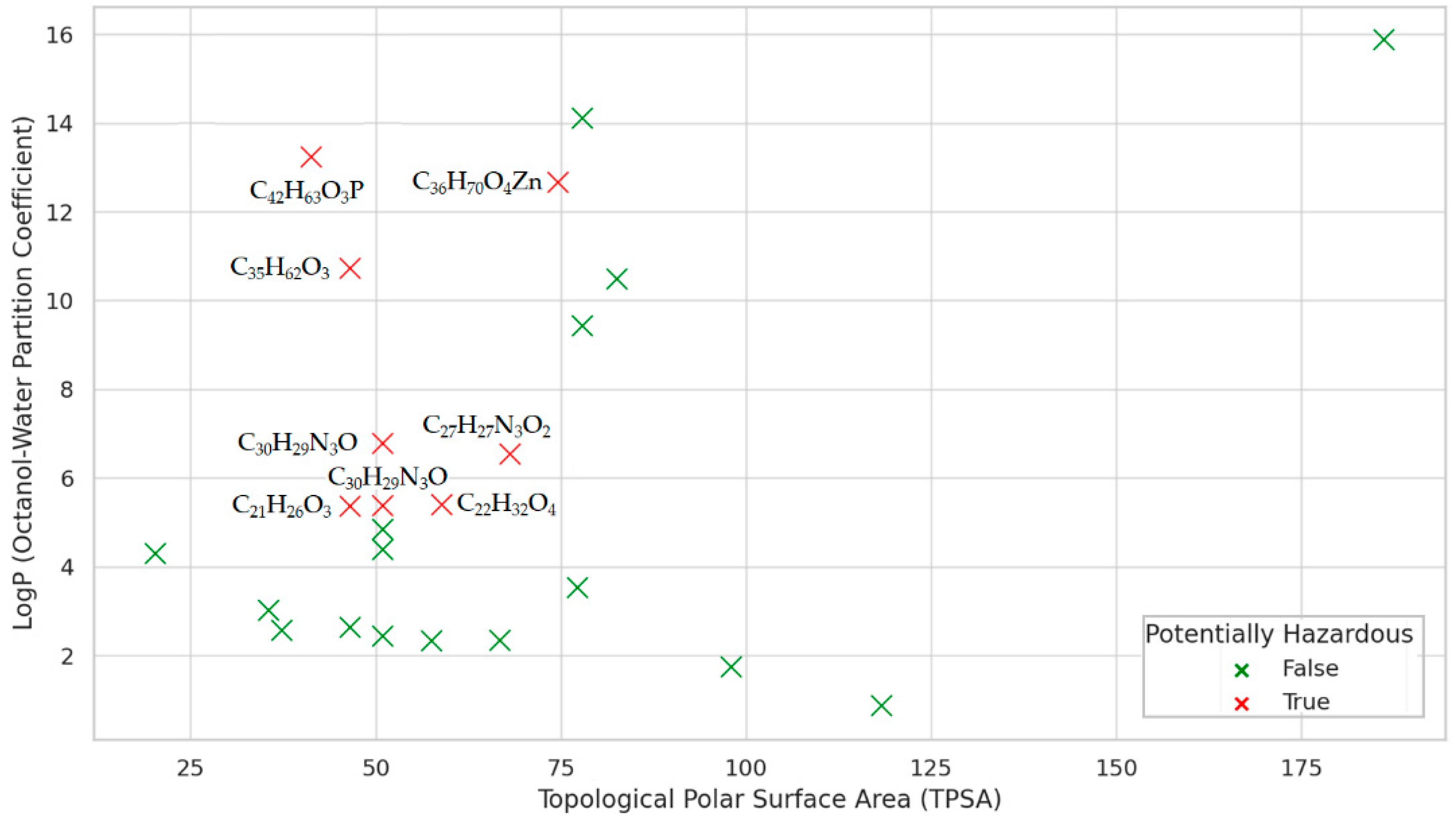
| CID | HBA | HBD | LogP | MR | TPSA | CID | HBA | HBD | LogP | MR | TPSA |
|---|---|---|---|---|---|---|---|---|---|---|---|
| 4632 | 15 | 1 | 2.6318 | 64.8315 | 46.53 | 62485 | 28 | 1 | 4.8399 | 99.1260 | 50.94 |
| 8569 | 16 | 2 | 2.3374 | 66.8545 | 66.76 | 62531 | 21 | 1 | 4.3854 | 90.1340 | 50.94 |
| 8571 | 15 | 4 | 1.7400 | 64.4085 | 57.99 | 64819 | 120 | 4 | 15.8792 | 348.9130 | 186.12 |
| 8572 | 13 | 2 | 2.3288 | 60.3625 | 57.53 | 70355 | 18 | 1 | 2.5645 | 59.7573 | 37.30 |
| 11178 | 75 | 2 | 12.6625 | 180.8236 | 74.60 | 77470 | 27 | 1 | 5.3745 | 104.4380 | 50.94 |
| 12738 | 87 | 0 | 14.1092 | 214.1690 | 77.90 | 90571 | 19 | 0 | 3.0151 | 72.7905 | 35.53 |
| 15797 | 29 | 1 | 5.3625 | 98.4805 | 46.53 | 91601 | 67 | 0 | 13.2353 | 203.7500 | 41.28 |
| 16386 | 65 | 1 | 10.7245 | 169.3960 | 46.53 | 93481 | 28 | 1 | 3.5292 | 100.8300 | 77.24 |
| 17113 | 14 | 1 | 2.4345 | 65.8540 | 50.94 | 112412 | 32 | 1 | 6.7779 | 138.7880 | 50.94 |
| 24667 | 36 | 2 | 5.3966 | 108.4540 | 58.92 | 172473 | 36 | 4 | 0.8663 | 86.9732 | 118.30 |
| 31250 | 63 | 0 | 9.4280 | 156.4850 | 77.90 | 3601357 | 62 | 0 | 10.4850 | 180.9930 | 82.56 |
| 31404 | 25 | 1 | 4.2956 | 71.9710 | 20.23 | 4992761 | 32 | 1 | 6.5373 | 128.6850 | 68.13 |
| CID | 4632 | 8569 | 8571 | 8572 | 11178 | 12738 | 15797 | 16386 | 17113 | 24667 | 31250 | 31404 | 62485 | 62531 | 77470 | 93481 | 112412 | 4992761 |
|---|---|---|---|---|---|---|---|---|---|---|---|---|---|---|---|---|---|---|
| 4632 | 1.00 | 0.76 | 0.42 | 0.70 | 0.42 | 0.33 | ||||||||||||
| 8569 | 1.00 | 0.55 | 0.60 | 0.35 | 0.33 | |||||||||||||
| 8571 | 1.00 | 0.57 | ||||||||||||||||
| 8572 | 1.00 | 0.36 | 0.33 | |||||||||||||||
| 11178 | 1.00 | 0.30 | 0.42 | |||||||||||||||
| 12738 | 1.00 | 0.52 | ||||||||||||||||
| 15797 | 1.00 | 0.34 | ||||||||||||||||
| 16386 | 1.00 | 0.30 | ||||||||||||||||
| 17113 | 1.00 | 0.44 | 0.44 | 0.30 | 0.32 | |||||||||||||
| 24667 | 1.00 | 0.45 | ||||||||||||||||
| 31250 | 1.00 | |||||||||||||||||
| 31404 | 1.00 | |||||||||||||||||
| 62485 | 1.00 | 0.43 | 0.42 | 0.41 | ||||||||||||||
| 62531 | 1.00 | 0.66 | 0.47 | 0.30 | ||||||||||||||
| 77470 | 1.00 | 0.44 | 0.37 | |||||||||||||||
| 93481 | 1.00 | |||||||||||||||||
| 112412 | 1.00 | |||||||||||||||||
| 4992761 | 1.00 |
| CID | 4632 | 8569 | 8571 | 8572 | 11178 | 12738 | 15797 | 16386 | 17113 | 24667 | 31250 | 31404 | 62485 | 62531 | 64819 | 70355 | 77470 | 90571 | 91601 | 93481 | 112412 | 172473 | 3601357 | 4992761 |
|---|---|---|---|---|---|---|---|---|---|---|---|---|---|---|---|---|---|---|---|---|---|---|---|---|
| 4632 | 1 | 1 | 0.94 | 1 | 0.18 | 0.18 | 1 | 0.53 | 0.47 | 0.53 | 0.18 | 0.56 | 0.53 | 0.53 | 0.59 | 0.6 | 0.53 | 0.53 | 0.53 | 0.53 | 0.82 | 0.18 | 0.53 | 0.59 |
| 8569 | 1 | 0.94 | 1 | 0.17 | 0.17 | 0.94 | 0.5 | 0.47 | 0.5 | 0.17 | 0.56 | 0.5 | 0.5 | 0.61 | 0.6 | 0.5 | 0.5 | 0.5 | 0.5 | 0.78 | 0.17 | 0.5 | 0.56 | |
| 8571 | 1 | 1 | 0.17 | 0.17 | 0.89 | 0.5 | 0.47 | 0.5 | 0.17 | 0.56 | 0.5 | 0.5 | 0.56 | 0.6 | 0.5 | 0.5 | 0.5 | 0.5 | 0.78 | 0.17 | 0.5 | 0.5 | ||
| 8572 | 1 | 0.19 | 0.19 | 1 | 0.56 | 0.5 | 0.56 | 0.19 | 0.56 | 0.56 | 0.56 | 0.63 | 0.6 | 0.56 | 0.56 | 0.56 | 0.56 | 0.88 | 0.19 | 0.56 | 0.56 | |||
| 11178 | 1 | 0.46 | 0.38 | 0.5 | 0.12 | 0.12 | 0.37 | 0.19 | 0.21 | 0.14 | 0.17 | 0.47 | 0.12 | 0.21 | 0.1 | 0.23 | 0.09 | 0.32 | 0.12 | 0.22 | ||||
| 12738 | 1 | 0.42 | 0.61 | 0.12 | 0.12 | 1 | 0.19 | 0.21 | 0.14 | 0.19 | 0.47 | 0.12 | 0.26 | 0.09 | 0.23 | 0.09 | 0.32 | 0.12 | 0.25 | |||||
| 15797 | 1 | 0.42 | 0.47 | 0.38 | 0.42 | 0.56 | 0.38 | 0.41 | 0.42 | 0.6 | 0.38 | 0.47 | 0.38 | 0.38 | 0.58 | 0.32 | 0.38 | 0.63 | ||||||
| 16386 | 1 | 0.47 | 0.42 | 0.49 | 1 | 0.42 | 0.55 | 0.61 | 0.6 | 0.56 | 0.47 | 0.37 | 0.65 | 0.41 | 0.32 | 0.42 | 0.25 | |||||||
| 17113 | 1 | 0.41 | 0.12 | 0.5 | 1 | 1 | 0.47 | 0.47 | 1 | 0.41 | 0.47 | 1 | 1 | 0.12 | 0.47 | 0.47 | ||||||||
| 24667 | 1 | 0.12 | 0.69 | 0.42 | 0.5 | 0.42 | 0.53 | 0.44 | 0.42 | 0.42 | 0.42 | 0.42 | 0.18 | 0.42 | 0.31 | |||||||||
| 31250 | 1 | 0.19 | 0.21 | 0.14 | 0.26 | 0.47 | 0.12 | 0.26 | 0.11 | 0.23 | 0.09 | 0.32 | 0.14 | 0.25 | ||||||||||
| 31404 | 1 | 0.63 | 0.75 | 1 | 0.53 | 0.88 | 0.5 | 0.88 | 0.75 | 0.88 | 0.25 | 1 | 0.5 | |||||||||||
| 62485 | 1 | 0.86 | 0.42 | 0.67 | 0.83 | 0.47 | 0.46 | 0.79 | 0.83 | 0.27 | 0.42 | 0.33 | ||||||||||||
| 62531 | 1 | 0.55 | 0.53 | 1 | 0.42 | 0.55 | 0.95 | 0.95 | 0.18 | 0.55 | 0.36 | |||||||||||||
| 64819 | 1 | 0.6 | 0.56 | 0.47 | 0.3 | 0.65 | 0.41 | 0.27 | 0.37 | 0.25 | ||||||||||||||
| 70355 | 1 | 0.53 | 0.73 | 0.6 | 0.6 | 0.53 | 0.47 | 0.6 | 0.47 | |||||||||||||||
| 77470 | 1 | 0.42 | 0.6 | 0.88 | 0.96 | 0.18 | 0.56 | 0.32 | ||||||||||||||||
| 90571 | 1 | 0.42 | 0.47 | 0.42 | 0.26 | 0.42 | 0.37 | |||||||||||||||||
| 91601 | 0.5 | 0.44 | 0.18 | 0.4 | 0.25 | |||||||||||||||||||
| 93481 | 1 | 0.85 | 0.27 | 0.46 | 0.31 | |||||||||||||||||||
| 112412 | 1 | 0.18 | 0.41 | 0.25 | ||||||||||||||||||||
| 172473 | 1 | 0.27 | 0.27 | |||||||||||||||||||||
| 3601357 | 1 | 0.25 | ||||||||||||||||||||||
| 4992761 | 1 |
| Stability | Internal | ||||
|---|---|---|---|---|---|
| (a) Run from two to four clusters | |||||
| Measures | Score | No of clusters | Measures | Score | No of clusters |
| AD | 0.7709 | 2 | Connectivity | 4.8409 | 2 |
| ADM | 0.0455 | 4 | Dunn | 0.6880 | 3 |
| APM | 0.0231 | 2 | Silhouette | 0.3969 | 4 |
| FOM | 0.1661 | 4 | |||
| (b) Run from two to six clusters | |||||
| Measures | Score | No of clusters | Measures | Score | No of clusters |
| AD | 0.5655 | 5 | Connectivity | 4.8409 | 2 |
| ADM | 0.0232 | 6 | Dunn | 0.7910 | 6 (k-means) |
| APM | 0.0089 | 6 | Silhouette | 0.3969 | 4 |
| FOM | 0.1175 | 6 | |||
| Cluster | Statistics | Tensile Strength (MPa) | Bending Elasticity Modulus (MPa) | Impact Resistance (kJ/m2) | Melting Flow Index (g/10 min) |
|---|---|---|---|---|---|
| CL1 | Min | 19.00 | 1100.00 | 3.20 | 2.30 |
| Max | 26.00 | 1375.00 | 4.30 | 3.10 | |
| Mean | 22.00 | 1218.75 | 3.68 | 2.65 | |
| Std.dev. | 2.55 | 105.14 | 0.42 | 0.30 | |
| CL2 | Min | 21.00 | 1180.00 | 3.50 | 2.60 |
| Max | 25.00 | 1300.00 | 4.10 | 3.00 | |
| Mean | 23.00 | 1235.00 | 3.78 | 2.80 | |
| Std.dev. | 1.41 | 43.30 | 0.22 | 0.14 | |
| CL3 | Min | 22.00 | 1230.00 | 3.60 | 2.70 |
| Max | 29.00 | 1450.00 | 4.60 | 3.50 | |
| Mean | 25.67 | 1341.67 | 4.13 | 3.10 | |
| Std.dev. | 2.50 | 83.29 | 0.37 | 0.29 | |
| CL4 | Min | 22.00 | 1185.00 | 3.50 | 2.60 |
| Max | 30.00 | 1500.00 | 5.00 | 3.50 | |
| Mean | 25.50 | 1332.50 | 4.18 | 2.98 | |
| Std.dev. | 2.95 | 110.44 | 0.52 | 0.32 |
| Cluster | Statistics | Tensile Strength (MPa) | Bending Elasticity Modulus (MPa) | Impact Resistance (kJ/m2) | Melting Flow Index (g/10 min) |
|---|---|---|---|---|---|
| CL1.1 | Value | 21.00 | 1150.00 | 3.40 | 2.50 |
| CL1.2 | Min | 19.00 | 1100.00 | 3.20 | 2.30 |
| Max | 26.00 | 1375.00 | 4.30 | 3.10 | |
| Mean | 22.33 | 1241.67 | 3.77 | 2.70 | |
| Std.dev. | 2.87 | 112.42 | 0.45 | 0.33 | |
| CL4.1 | Min | 25.00 | 1150.00 | 3.40 | 2.50 |
| Max | 30.00 | 1500.00 | 5.00 | 3.50 | |
| Mean | 27.50 | 1400.00 | 4.50 | 3.15 | |
| Std.dev. | 3.54 | 141.42 | 0.71 | 0.49 | |
| CL4.2 | Min | 22.00 | 1185.00 | 3.50 | 2.60 |
| Max | 28.00 | 1400.00 | 4.50 | 3.20 | |
| Mean | 24.50 | 1298.75 | 4.03 | 2.90 | |
| Std.dev. | 2.52 | 95.43 | 0.43 | 0.24 |
| Component | Description | Objective | References |
|---|---|---|---|
| Additive classification based on structural or functional similarity | Molecular descriptor-based clustering (e.g., FMCS, Tanimoto coefficient) | Enhancement of recycling formulations via the identification of additives with analogous behavior in polymers | [27,41,53] |
| Computation of descriptors (LogP, MR, HBA, HBD, TPSA) | Assessment of toxicological potential, molecular polarizability, and bioaccumulation capacity | Minimizing ecological and toxicological risks when choosing additives | [64,65,85] |
| Detection of high-performance mechanical clusters | Structure–property correlation with respect to key physico-mechanical parameters (e.g., MFI, elasticity) | Enhancement of the durability and lifespan of products and materials | [80,81,85] |
| Screening for additives with structural compatibility | Classification of additives according to their functional applicability (e.g., UV stabilizers, antioxidants) | Smart reuse strategies and function-driven design | [3,10,13] |
| Removal of potentially dangerous compounds (e.g., derivatives based on Cl, Zn, S) | Chemical structure and ecotoxicity-related molecular descriptors | Hazardous waste elimination and the promotion of alternative substitution | [11,12,94] |
Disclaimer/Publisher’s Note: The statements, opinions and data contained in all publications are solely those of the individual author(s) and contributor(s) and not of MDPI and/or the editor(s). MDPI and/or the editor(s) disclaim responsibility for any injury to people or property resulting from any ideas, methods, instructions or products referred to in the content. |
© 2025 by the authors. Licensee MDPI, Basel, Switzerland. This article is an open access article distributed under the terms and conditions of the Creative Commons Attribution (CC BY) license (https://creativecommons.org/licenses/by/4.0/).
Share and Cite
Bărbulescu, A.; Barbeș, L. Cheminformatics Approaches to the Analysis of Additives for Sustainable Polymeric Materials. Polymers 2025, 17, 1522. https://doi.org/10.3390/polym17111522
Bărbulescu A, Barbeș L. Cheminformatics Approaches to the Analysis of Additives for Sustainable Polymeric Materials. Polymers. 2025; 17(11):1522. https://doi.org/10.3390/polym17111522
Chicago/Turabian StyleBărbulescu, Alina, and Lucica Barbeș. 2025. "Cheminformatics Approaches to the Analysis of Additives for Sustainable Polymeric Materials" Polymers 17, no. 11: 1522. https://doi.org/10.3390/polym17111522
APA StyleBărbulescu, A., & Barbeș, L. (2025). Cheminformatics Approaches to the Analysis of Additives for Sustainable Polymeric Materials. Polymers, 17(11), 1522. https://doi.org/10.3390/polym17111522