Article

Selection of Network Parameters in Direct ANN Modeling of Roughness Obtained in FFF Processes

by
Irene Buj-Corral
1,*,
Maurici Sivatte-Adroer
2,
Lourdes Rodero-de-Lamo
3 and
Lluís Marco-Almagro
3
1
Department of Mechanical Engineering, Barcelona School of Industrial Engineering (ETSEIB), Universitat Politècnica de Catalunya, Av. Diagonal, 647, 08028 Barcelona, Spain
2
Department of Mechanical Engineering, Polytechnic School of Engineering of Vilanova i la Geltrú (EPSEVG), Universitat Politècnica de Catalunya, Av. Víctor Balaguer, 1, 08880 Vilanova i la Geltrú, Spain
3
Department of Statistics and Operations Research, Barcelona School of Industrial Engineering (ETSEIB), Universitat Politècnica de Catalunya, Av. Diagonal, 647, 08028 Barcelona, Spain
*
Author to whom correspondence should be addressed.
Polymers 2025, 17(1), 120; https://doi.org/10.3390/polym17010120
Submission received: 7 December 2024 / Revised: 27 December 2024 / Accepted: 3 January 2025 / Published: 6 January 2025

Abstract

:
Artificial neural network (ANN) models have been used in the past to model surface roughness in manufacturing processes. Specifically, different parameters influence surface roughness in fused filament fabrication (FFF) processes. In addition, the characteristics of the networks have a direct impact on the performance of the models. In this work, a study about the use of ANN to model surface roughness in FFF processes is presented. The main objective of the paper is discovering how key ANN parameters (specifically, the number of neurons, the training algorithm, and the percentage of training and validation datasets) affect the accuracy of surface roughness predictions. To address this question, 125 3D printing experiments were conducted changing orientation angle, layer height and printing temperature, and measuring average roughness Ra as response. A multilayer perceptron neural network model with backpropagation algorithm was used. The study evaluates the effect of three ANN parameters: (1) number of neurons in the hidden layer (4, 5, 6 or 7), (2) training algorithm (Levenberg–Marquardt, Resilient Backpropagation or Scaled Conjugate Gradient), and (3) data splitting ratios (70%–15%–15% vs. 55%–15%–30%). Mean Absolute Error (MAE) was used as the performance metric. The Resilient Backpropagation algorithm, 7 neurons, and using 55% of training data yielded the best predictive performance, minimizing the MAE. Additionally, the impact of the dataset size on prediction accuracy was analysed. It was observed that the performance of the ANN gets worse as the number of datasets is reduced, emphasizing the importance of having sufficient data. This study will help to select appropriate values for the printing parameters in FFF processes, as well as to define the characteristics of the ANN to be used to model surface roughness.

1. Introduction

Polylactic acid (PLA) is a biocompatible material that can be used in medical applications, for example to manufacture surgical models [1]. It can also be employed in tissue engineering, for instance to favor the integration of tissue-engineered bone with natural bone or to produce scaffolds to regenerate epithelial cells [2]. It allows obtaining biodegradable orthopedic devices [3]. Moreover, PLA is a bioresorbable polymer, commonly used for stents and sutures [4].
Fused Filament Fabrication (FFF), also known as Fused Deposition Modeling (FDM), consists of extruding material through a nozzle and depositing it to form a part layer by layer. Main advantages of this process are its easiness of use, its low cost if desktop technologies are employed, and the possibility to use different plastic materials [5]. Some of their drawbacks are its low dimensional accuracy [6,7] and its poor surface roughness in lateral walls [8], because of the ridge pattern which is formed by the beads’ edges.
Post-processing operations are often employed to reduce surface roughness of 3D printed parts. They can either be mechanical, chemical, thermal, or hybrid. For example, the surface peaks can be mechanically cut, pressed, or polished [9]. As for the chemical post-processing of plastic materials, for example acetone vapor is used in acrylonitrile butadiene styrene (ABS) parts [10]. Regarding thermal methods, for instance, laser polishing has been used in PLA parts to improve their surface finish [11]. However, post-processing methods could affect the structure and the mechanical properties of the parts [9]. Moreover, in addition to layer height, other 3D printing conditions can affect surface roughness. For example, for a certain layer height value, roughness increases in inclined walls due to the stair-stepping effect. Thus, print orientation angle has a great influence on roughness [12]. Hooshmand et al. [13] found that both build orientation and layer height have an important effect on surface roughness in FFF processes, with 0° and 0.22 mm, respectively, leading to optimal results. Similarly, Abas et al. [14] found lowest Ra values when build orientation values of 0° were selected, using I-optimal design and definitive screening design (DSD). In addition, printing temperature can affect roughness because it can lead to deformation of the deposited beads [15,16]. Specifically, roughness decreases when temperature increases from 210 °C to 230 °C in thin-walled PLA parts [17].
Artificial Neural Network (ANN) models have several advantages over regression or analytical models, such as their high computation, quick learning, and powerful memory [18]. Neural networks have been used in the past to model roughness in different manufacturing processes like milling [19] or honing [20]. In FFF processes, for example, Shirmohammadi et al. [21] employed ANN and particle swarm algorithm to model roughness in the lateral walls of the parts. They selected five process parameters, namely printing temperature, layer thickness, printing speed, nozzle diameter, and material density. They used a multi-layered perceptron neural network (7-4-1). They reported an error of 4.88%, while a surface response quadratic model with the same data showed an error of 8.75%. Tripathi and Singla [22] used ANN, with layer thickness, infill density, nozzle temperature, wall thickness, bed temperature, material, fan speed, print speed, and infill pattern as variables, and elongation, tensile strength and surface roughness as responses of the model. They used models with four layers.
As for the selection of best parameters of the networks, for example, Ke and Huang [23] combined systematic experimental design with ANN modeling in injection molding processes. They highlight the importance of selecting appropriate quality indices and optimizing neural network parameters to increase accuracy. For example, using the same number of neurons in the hidden layer as in the input layer provided quality training results. In FFF processes, Chinchanikar et al. [24] predicted surface roughness from different parameters, including number of neurons, number of hidden layers, layer height, infill density, nozzle temperature, and print speed. In this case, best results were obtained with two hidden layers and 150 neurons in each layer. However, when modeling FFF processes, there is little information in the literature about the neural network topology to be employed.
The main objective of the paper is discovering how key ANN parameters (specifically, the number of neurons, the training algorithm, and the percentage of training and validation datasets) affect the accuracy of surface roughness predictions in FFF processes. For this purpose, 125 3D printing experiments were conducted, changing print orientation angle, layer height, and printing temperature, and measuring average roughness Ra as response. A multilayer perceptron neural network model with a backpropagation algorithm is used. Finally, a study is performed to assess the effect of dataset size on the performance of the networks.

2. Materials and Methods

2.1. 3D Printing of the Samples

A Sigma R19 3D printer from BCN3D Technologies (Gavà, Spain) was used to print the samples (Figure 1).
Different cylindrical specimens of diameter 12.7 mm and height 25.4 mm were printed in Polylactic acid (PLA). The 3D printing parameters are presented in Table 1. In the experiments, nozzle diameter, infill ratio, and print speed were fixed, while print orientation angle (OA), layer height (LH), and printing temperature (PT) were varied, according to a 53 full factorial design. A total amount of 125 experiments was carried out (see Table A1 in Appendix A).
Nozzle diameter value of 0.4 mm and print speed value of 40 mm/s are usual in the FFF 3D printing of PLA. A high infill ratio of 80% was considered, so that high mechanical strength will be achieved. Print orientation angle covers the range between 0 and 80°. It excludes 90° (horizontal cylinder), which is a special case that provides low surface roughness values, since the measurement direction is parallel to the printed layers [12]. Layer height covers a wide range of values from 0.05 mm to 0.25 mm, all of them below the nozzle diameter value of 0.4 mm. Printing temperature ranges between 190 °C and 210 °C, which are usual when 3D printing PLA [25]. Similar values were used by Kugunavar et al. [26] for print orientation angle, layer height, and printing temperature, when analyzing roughness with the Taguchi method.
Figure 2 shows two different specimens obtained with layer inclination 50° (left) and 10° (right), corresponding to print orientation 40° (left) and 80° (right).

2.2. Roughness Measurement

Roughness was measured with a Talysurf 2 (Taylor Hobson Ltd., Leicester, UK) contact roughness meter. The samples were placed on V-shaped blocks. A diamond tip was used with tip radius of 2 µm. Resolution of the inductive sensor is 18 nm.
Roughness profiles were measured along a generatrix of the samples (red line in Figure 2), which corresponds to their lateral walls. Specifically, the generatrix was measured that is placed opposite to the printing supports. For print orientation angle of 0° (vertical cylinder), no printing supports are required and a random generatrix of the part is measured. In this case, the measurement direction is perpendicular to the printing layers.
A Gaussian filter was considered with a cut-off length of 0.8 mm and an evaluation length of 4 mm. The average roughness parameter Ra was determined from the roughness profiles.

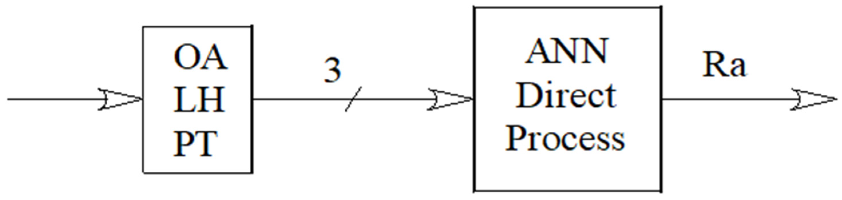
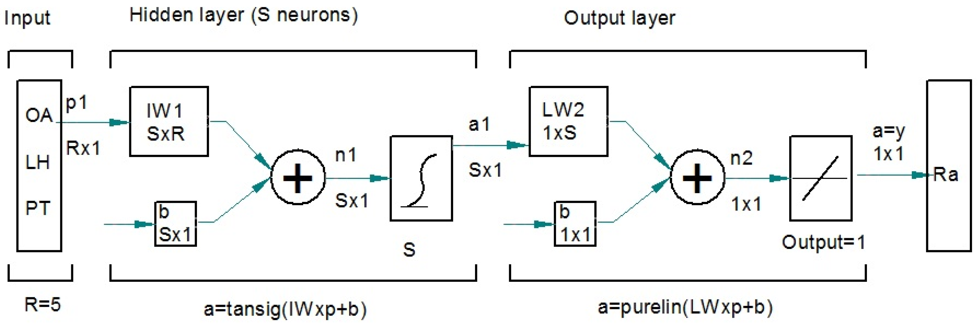
2.3. Neural Networks

Figure 3 shows a schematic diagram of the network employed, in which the direct problem is addressed. It has three inputs, namely print orientation angle (OA), layer height (LH), and printing temperature (PT), and one output, average roughness Ra.
The detailed structure of the network is provided in Figure 4.
The ANN is based on a feed forward multilayer perceptron, with a backpropagation algorithm, having 3 input variables, OA, LH, and PT, one hidden layer with sigmoidal function and one output layer with one neuron and linear function. The network has one output variable, roughness parameter Ra. The multilayer perceptron has been proven to be a universal approximator [27].
A database with 125 datasets was used. It was randomly divided into two groups: a first group of datasets for training and validation of the networks, and a second group of datasets to test the results, in order to assess the goodness of the selected network. In order to compare the behavior of the different networks, the Mean Absolute Error (MAE) of the test data, in µm, was used (Equation (1)).
M A E = | O b j e c t i v e   o u t p u t S i m u l a t e d   o u t p u t | N u m b e r   o f   d a t a s e t s
where,
Objective output is the measured Ra value, in µm,
Simulated output is the Ra value provided by a network, in µm,
Number of datasets is the total number of datasets, in this case 125.
In order to assess the effect of the ANN parameters on MAE, different ANN models were obtained, in which three factors were varied:
  • Number of neurons in the hidden layer (4 levels).
  • Training algorithm used (3 levels).
  • Distribution of the dataset patterns among training, validation and test data (2 levels).
There are 24 sets of networks because this is the result of all combinations of 4 levels for the number of neurons (4, 5, 6 and 7), 3 levels for the training algorithm (LM, RB and SCG), and 2 levels for the distribution of datasets (70% train + 15% validation, 55% train + 30% validation). This is a full factorial design on the created networks (4 × 3 × 2 = 24).
Each factor of the networks is explained in detail in the next subsections.

2.3.1. Number of Neurons in the Hidden Layer

In order to define the range of values for the number of neurons to be tested, the starting point was the work by Lawrence and Peterson [28] and Feng et al. [29], where they optimize the number of neurons in the hidden layer as the summation of the number of inputs and outputs. Thus, with the start point of 4 neurons in the hidden layer, corresponding to 3 inputs and 1 output, different number of neurons were tested (Table 2).

2.3.2. Training Algorithm

A second factor that defines the networks is the training algorithm. Three different algorithms were selected and tested, which are usually employed in models with multilayer perceptron with backpropagation algorithm (Table 3).

2.3.3. Distribution of Datasets

A third factor that configures the training process of the network is the distribution of datasets among the training, validation, and test datasets. According to different studies [30,31], and depending on the number of experiments performed and the degree of complexity of the problem, the following ranges are recommended:
Training data between 50 and 70%.
Validation data between 15 and 25%.
Test data between 15 and 25%.
In this study, the test data are used to compare the different networks. For this reason, the same test data are used in all cases. Thus, the percentage of test datasets is defined as 15%, and the rest of the datasets, 85%, are used to train and validate the networks, according to the following distributions of datasets or datasets splitting ratios (Table 4).

3. Results and Discussion

Table A1 in the Appendix A shows the experimental Ra values for the 125 3D printing experiments that were carried out.

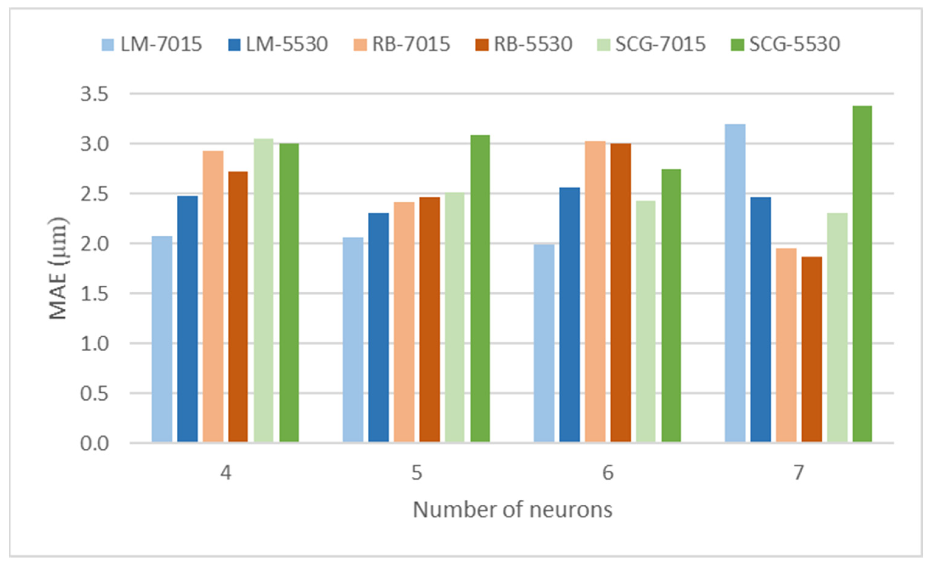
3.1. Study About Different Networks

Using the experimental results for the 125 experiments, 24 different networks were tested, according to the definition in Section 2.3.1. The MAE values of the networks are presented in Table 5. The name of each network consists of the acronym of the training algorithm followed by the number of neurons and the dataset distribution. For instance, LM-4-7015 corresponds to the Levenberg–Marquardt algorithm, with four neurons in the hidden layer, and with 70–15% data splitting ratios.
Figure 5 depicts the MAE values for the different combinations of training algorithm and dataset distribution, as a function of the number of neurons in the hidden layer.
Table 5 and Figure 5 show that, as a general trend, when four, five, or six neurons are considered, LM models provide lower MAE values than RB and SCG models. However, when seven neurons are used, RB models lead to lower values than the other models. Specifically, the best results are obtained with the RB algorithm, seven neurons and a distribution of 55% training data, 30% validation data, and 15% test data, with MAE of 1.874 µm (network 16). A similar number of neurons in the hidden layer, eight, was reported by Sood et al. [32] to model the compressive strength of parts in FFF processes, with a model having five input variables: layer thickness, orientation, raster angle, raster width, and air gap. Similarly, Saad et al. [33] selected eight neurons in each one of the two hidden layers of their model for roughness, with four input variables: layer thickness, print speed, print temperature, and outer shell speed. On the contrary, other authors used models with a higher number of neurons, for example 150, in a model with six input variables [24]. As for the algorithm, different options are available in FFF processes. For example, Mahapatra et al. used the Levenberg–Marquardt one [34], with the advantage of the faster training of ANN. Other authors like Monticeli et al. [35] employed the Resilient Backpropagation algorithm in order to predict the bending properties of FDM printed parts. Hosseini et al. [36] used the Scaled Conjugate Gradient backpropagation algorithm, together with the Levenberg–Marquardt algorithm and the Bayesian regularization in ANN combined with the genetic algorithm, in order to model the behavior of sinusoidal structures under quasi-static loading. They found that the Levenberg–Marquardt algorithm depended less on the number of neurons than the other algorithms did. In this work, LM models with four, five, and six neurons provided similar MAE values, while higher MAE values were obtained when seven neurons and the 7015 distribution were selected (network 7, LM-7-7015). On the other hand, increasing the number of training datasets does not always lead to lower error [36]. Similarly, in this work, in some cases using 70% of training datasets implies a higher error than using 55% of training datasets (for example, network 9, RB-4-7015, leads to higher error than network 10, RB-4-5530).

3.2. Optimization of Simulated Ra Values

In order to optimize roughness, the lowest simulated Ra values were searched among the 125 datasets. In Table 6, the lowest simulated Ra values for network 16 are presented.
The lowest simulated Ra values correspond to the low print orientation angle of 0° and the low layer height of 0.05 mm, with a high printing temperature equal or higher than 200 °C. Thus, in order to minimize surface roughness, a low orientation angle and a low layer height need to be selected, with a relatively high printing temperature.

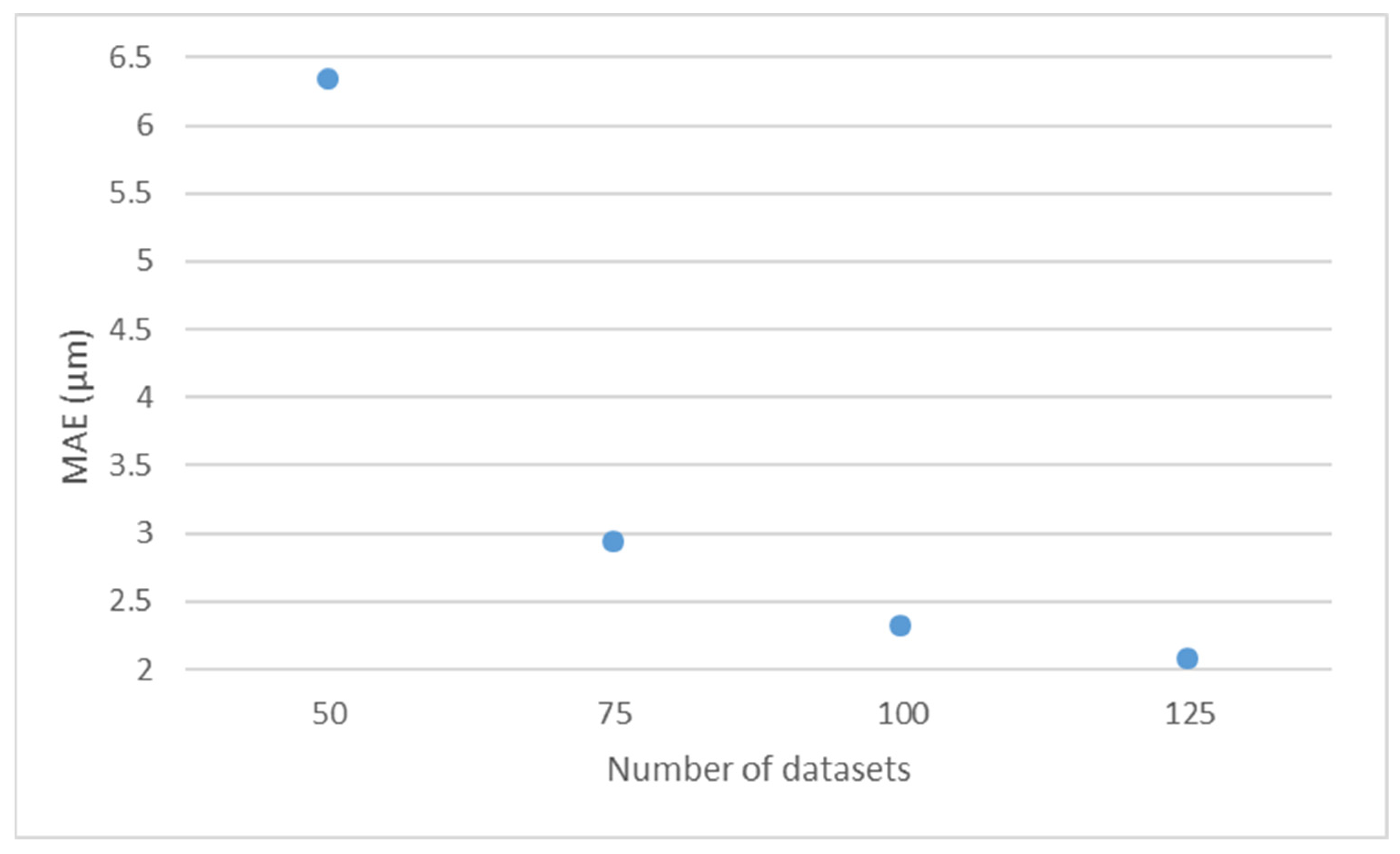
3.3. Study About the Database Size

In the study, network number 3 was selected, LM-5-7015, with the LM learning algorithm, five neurons in the hidden layer and a structure of 70% training datasets, 15% validation datasets, and 15% test datasets. According to Table 5, it provided a MAE value for the test data of 2.068 μm, which is in the middle range for MAE.
The database size or total number of datasets is a key parameter for the configuration of neural networks [37]. In order to evaluate its influence on the performance of the networks, first, the 19 test datasets were separated from the 125 datasets. Then, four different configurations with different total number of datasets were selected, according to Table 7.
A is the original configuration, with 106 training datasets and a total amount of 125 datasets. Configurations B, C, and D correspond to 81, 56, and 31 training datasets, with a total amount of 100, 75, and 50 datasets, respectively.
The selected network was trained with the different number of training datasets that are defined in Table 7. In configurations B, C and D, the training was repeated three times, with a different random selection of the training datasets and the validation datasets.
Finally, the MAE values were calculated for each configuration. The results are presented in Table 8.
It is observed that, the lower the number of total datasets, the higher the average MAE of the networks.
Figure 6 shows MAE as a function of total number of datasets. It is observed that, when the total number of datasets increases from 50 (configuration D) to 75 (configuration C), the average MAE of the network decreases substantially.
Thus, the higher the number of total datasets, the better the simulation is. Moreover, when the number of total datasets decreases to below 50, the network loses its effectivity.

4. Conclusions

Regarding the different neural network configuration studied, the main conclusions are as follows:
When a low number of neurons is selected (either four, or five), the LM algorithm provides better results than the other algorithms. However, lowest error among the networks studied corresponds to seven neurons, RB algorithm and 5530 distribution. According to this network, Ra values are minimized when a low orientation angle of 0°, a low layer height of 0.05 mm, and a relatively high printing temperature above 200 °C are selected.
The RB training algorithm is less sensitive to the relative variation of the train and validation data than the other algorithms tested, with similar results for 70% training datasets and for 55% training datasets. On the contrary, as a general trend, LM and SCG training algorithms behave better when 70% training datasets are selected, except for four neurons with the SCG algorithm and seven neurons with the LM algorithm.
Regarding the size of the total database, the lower the number of datasets, the higher the error of the network, with a sharp increase in MAE when 50 datasets are considered.
This work will help to select appropriate ANN parameters in order to reduce roughness in FFF processes. It will also contribute to the definition of efficient ANN models, which can be used in industry to optimize the 3D printing parameters from the experimental roughness values.
Although the main parameters in the ANN configuration have been considered in this study, future research directions could include other ANN parameters such as the type of functions employed. In addition, the same or similar prediction models could be tested to study other responses such as the dimensional accuracy of porosity of the 3D-printed parts.

Author Contributions

Conceptualization, I.B.-C. and M.S.-A.; methodology, I.B.-C., M.S.-A., L.R.-d.-L. and L.M.-A.; software, M.S.-A. and L.R.-d.-L.; validation, I.B.-C., L.M.-A. and M.S.-A.; formal analysis, I.B.-C.; investigation I.B.-C. and M.S.-A.; resources, I.B.-C.; data curation, I.B.-C., M.S.-A., L.R.-d.-L. and L.M.-A.; writing—original draft preparation, M.S.-A.; writing—review and editing, I.B.-C.; visualization, L.R.-d.-L. and L.M.-A.; supervision, I.B.-C. and L.R.-d.-L.; project administration, I.B.-C.; funding acquisition, I.B.-C. All authors have read and agreed to the published version of the manuscript.

Funding

This research was funded by the Spanish Research Agency, project number PID2020-115647RB-C21.

Institutional Review Board Statement

Not applicable.

Data Availability Statement

The data presented in this study are available on request from the corresponding author.

Acknowledgments

The authors would like to thank Alejandro Domínguez and Ramón Casado for their help with the experimental tests. They also thank the Catalan Government for the quality accreditation given to the research group TECNOFAB (2021 SGR 01034). TECNOFAB belongs to the group DIGIFACT, which is a certified agent TECNIO in the category of technology developers from the Government of Catalonia.

Conflicts of Interest

The authors declare no conflicts of interest.

Appendix A

Table A1 contains the measured Ra values for the different experiments performed.
Table A1. Ra values for the 125 experiments.
ExperimentLayer Height (mm)Temperature (°C)Print Orientation Angle (°)Ra (μm)
10.0519004.770
20.151908018.212
30.102006016.136
40.151954016.468
50.051958012.385
60.20205015.747
70.202054022.477
80.052058010.675
90.151906022.737
100.152008017.327
110.05210609.804
120.202004021.613
130.251908017.120
140.202002015.088
150.20190015.019
160.152056023.517
170.252052019.199
180.101902010.207
190.101958017.068
200.102106018.352
210.152058017.186
220.251904026.255
230.0520505.377
240.051956010.702
250.052008011.011
260.152052013.087
270.252008014.195
280.101906015.856
290.05210205.123
300.05190609.715
310.152102010.966
320.252054028.782
330.25195018.608
340.102004013.320
350.202108013.319
360.201908018.059
370.202006025.140
380.252106032.130
390.20200014.623
400.25190017.659
410.0520003.8395
420.102008015.957
430.15210010.404
440.251954029.163
450.252108017.306
460.20195014.640
470.202102015.477
480.25210017.429
490.102058014.565
500.051908010.966
510.05210409.816
520.251958014.261
530.1019506.968
540.152106024.996
550.201902015.450
560.15205010.067
570.152004018.815
580.252104028.472
590.202058015.486
600.152054018.014
610.152108015.073
620.152104018.563
630.151958015.829
640.201956030.767
650.10205209.166
660.052108011.414
670.05205609.971
680.251902021.956
690.201958021.739
700.1020507.154
710.252102019.904
720.252006030.778
730.201954026.123
740.102104012.475
750.05190408.538
760.10200208.093
770.10210208.470
780.101954012.415
790.151904024.313
800.251952030.005
810.15195010.074
820.052054011.703
830.202056024.597
840.101904016.937
850.05200609.490
860.252058028.090
870.05200207.186
880.251956048.851
890.0521003.880
900.202052021.630
910.252002027.833
920.1019006.609
930.101908021.895
940.202106029.740
950.202008032.232
960.05195409.922
970.151902018.600
980.1021006.792
990.151956033.355
1000.252056045.503
1010.25205018.356
1020.0519504.252
1030.202104036.138
1040.152002016.747
1050.152006025.378
1060.201904033.423
1070.15200011.104
1080.05200407.987
1090.20210014.775
1100.05195206.834
1110.201906040.021
1120.102056024.393
1130.102054018.439
1140.05205207.736
1150.151952011.570
1160.1519009.994
1170.25200017.590
1180.10195208.327
1190.1020006.645
1200.102108013.600
1210.201952014.002
1220.05190207.576
1230.252004030.875
1240.101956016.863
1250.251906055.106

References

  1. Werz, S.M.; Zeichner, S.J.; Berg, B.I.; Zeilhofer, H.F.; Thieringer, F. 3D Printed Surgical Simulation Models as Educational Tool by Maxillofacial Surgeons. Eur. J. Dent. Educ. 2018, 22, e500–e505. [Google Scholar] [CrossRef] [PubMed]
  2. DeStefano, V.; Khan, S.; Tabada, A. Applications of PLA in Modern Medicine. Eng. Regen. 2020, 1, 76–87. [Google Scholar] [CrossRef]
  3. Pawar, R.P.; Tekale, S.U.; Shisodia, S.U.; Totre, J.T.; Domb, A.J. Biomedical Applications of Poly (Lactic Acid). Recent Pat. Regen. Med. 2014, 4, 40–51. [Google Scholar] [CrossRef]
  4. Bergström, J.S.; Hayman, D. An Overview of Mechanical Properties and Material Modeling of Polylactide (PLA) for Medical Applications. Ann. Biomed. Eng. 2016, 44, 330–340. [Google Scholar] [CrossRef] [PubMed]
  5. Gibson, I.; Rosen, D.; Stucker, B. Additive Manufacturing Technologies: 3D Printing, Rapid Prototyping, and Direct Digital Manufacturing, 2nd ed.; Springer: New York, NY, USA, 2015; ISBN 9781493921133. [Google Scholar]
  6. Buj-Corral, I.; Zayas-Figueras, E.E. Comparative Study about Dimensional Accuracy and Form Errors of FFF Printed Spur Gears Using PLA and Nylon. Polym. Test. 2022, 117, 107862. [Google Scholar] [CrossRef]
  7. Vidakis, N.; David, C.; Petousis, M.; Sagris, D.; Mountakis, N.; Moutsopoulou, A. The Effect of Six Key Process Control Parameters on the Surface Roughness, Dimensional Accuracy, and Porosity in Material Extrusion 3D Printing of Polylactic Acid: Prediction Models and Optimization Supported by Robust Design Analysis. Adv. Ind. Manuf. Eng. 2022, 5, 100104. [Google Scholar] [CrossRef]
  8. Kechagias, J.; Chaidas, D.; Vidakis, N.; Salonitis, K.; Vaxevanidis, N.M. Key Parameters Controlling Surface Quality and Dimensional Accuracy: A Critical Review of FFF Process. Mater. Manuf. Process. 2022, 37, 963–984. [Google Scholar] [CrossRef]
  9. Mathew, A.; Kishore, S.R.; Tomy, A.T.; Sugavaneswaran, M.; Scholz, S.G.; Elkaseer, A.; Wilson, V.H.; John Rajan, A. Vapour Polishing of Fused Deposition Modelling (FDM) Parts: A Critical Review of Different Techniques, and Subsequent Surface Finish and Mechanical Properties of the Post-Processed 3D-Printed Parts. Prog. Addit. Manuf. 2023, 8, 1161–1178. [Google Scholar] [CrossRef]
  10. Neff, C.; Trapuzzano, M.; Crane, N.B. Impact of Vapor Polishing on Surface Quality and Mechanical Properties of Extruded ABS. Rapid Prototyp. J. 2018, 24, 501–508. [Google Scholar] [CrossRef]
  11. Chai, Y.; Li, R.W.; Perriman, D.M.; Chen, S.; Qin, Q.H.; Smith, P.N. Laser Polishing of Thermoplastics Fabricated Using Fused Deposition Modelling. Int. J. Adv. Manuf. Technol. 2018, 96, 4295–4302. [Google Scholar] [CrossRef]
  12. Buj-Corral, I.; Domínguez-Fernández, A.; Durán-Llucià, R. Influence of Print Orientation on Surface Roughness in Fused Deposition Modeling (FDM) Processes. Materials 2019, 12, 3834. [Google Scholar] [CrossRef] [PubMed]
  13. Hooshmand, M.J.; Mansour, S.; Dehghanian, A. Optimization of Build Orientation in FFF Using Response Surface Methodology and Posterior-Based Method. Rapid Prototyp. J. 2021, 27, 967–994. [Google Scholar] [CrossRef]
  14. Abas, M.; Habib, T.; Noor, S.; Khan, K.M. Comparative Study of I-Optimal Design and Definitive Screening Design for Developing Prediction Models and Optimization of Average Surface Roughness of PLA Printed Parts Using Fused Deposition Modeling. Int. J. Adv. Manuf. Technol. 2023, 125, 689–700. [Google Scholar] [CrossRef]
  15. Vasudevarao, B.; Natarajan, D.P.; Henderson, M. Sensitivity of Rp Surface Finish to Process. In Proceedings of the International Solid Freeform Fabrication Symposium, Austin, TX, USA, 8–10 August 2000; pp. 251–258. [Google Scholar]
  16. Ding, S.; Zou, B.; Wang, P.; Ding, H. Effects of Nozzle Temperature and Building Orientation on Mechanical Properties and Microstructure of PEEK and PEI Printed by 3D-FDM. Polym. Test. 2019, 78, 105948. [Google Scholar] [CrossRef]
  17. Aslani, K.E.; Chaidas, D.; Kechagias, J.; Kyratsis, P.; Salonitis, K. Quality Performance Evaluation of Thinwalled PLA 3D Printed Parts Using the Taguchi Method and Grey Relational Analysis. J. Manuf. Mater. Process. 2020, 4, 47. [Google Scholar] [CrossRef]
  18. Chowdhury, S.; Mhapsekar, K.; Anand, S. Part Build Orientation Optimization and Neural Network-Based Geometry Compensation for Additive Manufacturing Process. J. Manuf. Sci. Eng. Trans. ASME 2018, 140, 031009. [Google Scholar] [CrossRef]
  19. Zain, A.M.; Haron, H.; Sharif, S. Prediction of Surface Roughness in the End Milling Machining Using Artificial Neural Network. Expert Syst. Appl. 2010, 37, 1755–1768. [Google Scholar] [CrossRef]
  20. Sivatte-Adroer, M.; Llanas-Parra, X.; Buj-Corral, I.; Vivancos-Calvet, J. Indirect Model for Roughness in Rough Honing Processes Based on Artificial Neural Networks. Precis. Eng. 2016, 43, 505–513. [Google Scholar] [CrossRef]
  21. Shirmohammadi, M.; Goushchi, S.J.; Keshtiban, P.M. Optimization of 3D Printing Process Parameters to Minimize Surface Roughness with Hybrid Artificial Neural Network Model and Particle Swarm Algorithm. Prog. Addit. Manuf. 2021, 6, 199–215. [Google Scholar] [CrossRef]
  22. Tripathi, A.; Singla, R. Surface Roughness Prediction of 3D Printed Surface Using Artificial Neural Networks. In Advances in Interdisciplinary Engineering: Select Proceedings of FLAME 2020; Lecture Notes in Mechanical Engineering; Springer: Singapore, 2021; pp. 109–120. [Google Scholar] [CrossRef]
  23. Ke, K.C.; Huang, M.S. Quality Prediction for Injection Molding by Using a Multilayer Perceptron Neural Network. Polymers 2020, 12, 1812. [Google Scholar] [CrossRef] [PubMed]
  24. Chinchanikar, S.; Shinde, S.; Gaikwad, V.; Shaikh, A.; Rondhe, M.; Naik, M. ANN Modelling of Surface Roughness of FDM Parts Considering the Effect of Hidden Layers, Neurons, and Process Parameters. Adv. Mater. Process. Technol. 2024, 10, 22–32. [Google Scholar] [CrossRef]
  25. Lokesh, N.; Praveena, B.A.; Sudheer Reddy, J.; Vasu, V.K.; Vijaykumar, S. Evaluation on Effect of Printing Process Parameter through Taguchi Approach on Mechanical Properties of 3D Printed PLA Specimens Using FDM at Constant Printing Temperature. Mater. Today Proc. 2022, 52, 1288–1293. [Google Scholar] [CrossRef]
  26. Kugunavar, S.; Viralka, M.; Sangwan, K.S. Development of a Hybrid Model to Estimate Surface Roughness of 3D Printed Parts. Addit. Manuf. 2024, 92, 104368. [Google Scholar] [CrossRef]
  27. Hornik, K.; Stinchcombe, M.; White, H. Multilayer Feedforward Networks Are Universal Approximators. Neural Netw. 1989, 2, 359–366. [Google Scholar] [CrossRef]
  28. Lawrence, M.; Petterson, A. Getting Started with Brain Maker: Neural Network Simulation Software User’s Guide and Reference Manual/Introduction to Neural Networks and Disk [Hardcover]; Bks&Disk edition; California Scientific Software: Pleasanton, CA, USA, 1990; ISBN 9991846883. [Google Scholar]
  29. Feng, C.-X.; Wang, X.; Yu, Z. Neural Networks Modeling of Honing Surface Roughness Parameters Defined by ISO 13565. J. Manuf. Syst. 2002, 21, 395–408. [Google Scholar] [CrossRef]
  30. Crowther, P.S.; Cox, R.J. A Method for Optimal Division of Data Sets for Use in Neural Networks. In Knowledge-Based Intelligent Information and Engineering Systems (KES 2005); Lecture Notes in Computer Science; Springer: Berlin/Heidelberg, Germany, 2005; Volume 3684, pp. 1–7. [Google Scholar]
  31. Guyon, I. A Scaling Law for the Validation-Set Training-Set Size Ratio. ATT Bell Lab. 1997, 1. [Google Scholar]
  32. Sood, A.K.; Ohdar, R.K.; Mahapatra, S.S. Experimental Investigation and Empirical Modelling of FDM Process for Compressive Strength Improvement. J. Adv. Res. 2012, 3, 81–90. [Google Scholar] [CrossRef]
  33. Saad, M.S.; Mohd Nor, A.; Abd Rahim, I.; Syahruddin, M.A.; Mat Darus, I.Z. Optimization of FDM Process Parameters to Minimize Surface Roughness with Integrated Artificial Neural Network Model and Symbiotic Organism Search. Neural Comput. Appl. 2022, 34, 17423–17439. [Google Scholar] [CrossRef]
  34. Mahapatra, S.S.; Sood, A.K. Bayesian Regularization-Based Levenberg-Marquardt Neural Model Combined with BFOA for Improving Surface Finish of FDM Processed Part. Int. J. Adv. Manuf. Technol. 2012, 60, 1223–1235. [Google Scholar] [CrossRef]
  35. Monticeli, F.M.; Neves, R.M.; Ornaghi, H.L.; Almeida, J.H.S. Prediction of Bending Properties for 3D-Printed Carbon Fibre/Epoxy Composites with Several Processing Parameters Using ANN and Statistical Methods. Polymers 2022, 14, 3668. [Google Scholar] [CrossRef]
  36. Hosseini, S.; Farrokhabadi, A.; Chronopoulos, D. Experimental and Numerical Analysis of Shape Memory Sinusoidal Lattice Structure: Optimization through Fusing an Artificial Neural Network to a Genetic Algorithm. Compos. Struct. 2023, 323, 117454. [Google Scholar] [CrossRef]
  37. Beresford, R.; Agatonovic-Kustrin, S. Basic Concepts of Artificial Neural Network (ANN) Modeling and Its Application in Pharmaceutical Research. J. Pharm. Biomed. Anal. 2000, 22, 717–727. [Google Scholar]
Figure 1. Sigma R19 3D printer.
Polymers 17 00120 g001
Figure 2. Three-dimensional printed cylinders with print orientation angle 40° (left) and 80° (right).
Polymers 17 00120 g002
Figure 3. Schematic diagram of the ANN employed.
Polymers 17 00120 g003
Figure 4. Structure of the ANN employed.
Polymers 17 00120 g004
Figure 5. MAE values for the different network structures.
Polymers 17 00120 g005
Figure 6. Average MAE values for the different number of datasets.
Polymers 17 00120 g006
Table 1. 3D printing parameters.
ParameterValue
Nozzle diameter (mm)0.4
Infill ratio (%)80
Print speed (mm/s)40
Print orientation angle (°) (OA)0, 20, 40, 60, and 80
Layer height (mm) (LH)0.05, 0.10, 0.15, 0.20, and 0.25
Printing temperature (°C) (PT)190, 195, 200, 205, and 210
Table 2. Number of neurons in the hidden layer.
Number of Neurons in the Hidden Layer
4567
Table 3. Training algorithm.
Training Algorithm
Levenberg–Marquardt
(LM)
Resilient-Backpropagation (RB)Scaled Conjugate Gradient (SCG)
Table 4. Distribution of datasets.
Distribution of Datasets
70% train + 15% validation
(7015)
55% train + 30% validation
(5530)
Table 5. MAE values for the different networks.
Network Nr.Network NameMAE (µm)
1LM-4-70152.075
2LM-4-55302.477
3LM-5-70152.068
4LM-5-55302.309
5LM-6-70151.997
6LM-6-55302.569
7LM-7-70153.203
8LM-7-55302.470
9RB-4-70152.926
10RB-4-55302.718
11RB-5-70152.417
12RB-5-55302.463
13RB-6-70153.024
14RB-6-55303.009
15RB-7-70151.953
16RB-7-55301.874
17SCG-4-70153.048
18SCG-4-55303.006
19SCG-5-70152.514
20SCG-5-55303.088
21SCG-6-70152.425
22SCG-6-55302.749
23SCG-7-70152.315
24SCG-7-55303.381
Table 6. Lowest Ra values among all datasets, simulated with network 16.
ExperimentOA (°)LH (mm)PT (°C)Simulated Ra (µm)
8900.052102.802
2300.052053.040
4100.052003.678
Table 7. Number of datasets for the different configurations.
ConfigurationTotal DatasetsTest DatasetsTraining Datasets
A12519106
B1001981
C751956
D501931
Table 8. MAE values for each configuration.
ConfigurationMAE (µm)Average MAE (µm)
A2.0682.068
B_12.1472.312
B_22.197
B_32.594
C_13.5942.940
C_22.565
C_32.661
D_17.6176.347
D_26.447
D_34.977
Disclaimer/Publisher’s Note: The statements, opinions and data contained in all publications are solely those of the individual author(s) and contributor(s) and not of MDPI and/or the editor(s). MDPI and/or the editor(s) disclaim responsibility for any injury to people or property resulting from any ideas, methods, instructions or products referred to in the content.

