

Cyclic Thermomechanical Loading of Epoxy Polymer: Modeling with Consideration of Stress Accumulation and Experimental Verification


Abstract
1. Introduction
- Determine the mechanical parameters of the epoxy polymer being studied for the viscoelastic structural model Kelvin–Voigt.
- Develop a methodology and conduct experimental studies on the stress state of the investigated polymer under the combined effects of static mechanical load and cyclic changes in temperature.
- Model the effects of cyclic thermomechanical loading on the epoxy polymer, using the proposed structural model, in conditions that correspond to the experiment.
- Compare the results of the stress state modeling with the experimental outcomes.
- It includes experimental data that expose the patterns of epoxy polymer’s stress state formation under cyclic thermomechanical loading.
- It shows the results from modeling the stress condition of epoxy polymers under repeated thermomechanical loading and compares them with experimental data.
2. Materials and Methods
2.1. Materials
- -
- KER 828 epoxy resin: epoxy group content (EGC) 5308 mmol/kg, equivalent epoxy weight (EEW) 188.5 g/eq, viscosity at 25 °C 12.7 Pa × s, HCl 116 mg/kg, total chlorine 1011 mg/kg. Manufacturer: KUMHO P&B Chemicals, Seoul, Korea.
- -
- Isomethyltetrahydrophthalic anhydride (IZOMTGFA) (hardener for epoxy resin): viscosity at 25 °C 63 Pa × s, anhydride content 42.4%, volatile fraction content 0.55%, free acid 0.1%. Manufacturer: ASAMBLY Chemicals Company Ltd., Nanjing, China.
- -
- Alkophen (epoxy curing booster): viscosity at 25 °C 150 Pa × s, molecular formula C15H27N3O, molecular weight 265, amine number 600 mg KOH/g. Manufacturer: JSC “Epital”, Moscow, Russian Federation.
- -
- Epoxy resin (KER 828)—52.5%.
- -
- Hardener (IZOMTGFA)—44.5%.
- -
- Curing booster (Alkophen)—3%.
2.2. Methods
2.2.1. Methods of Experimental Research
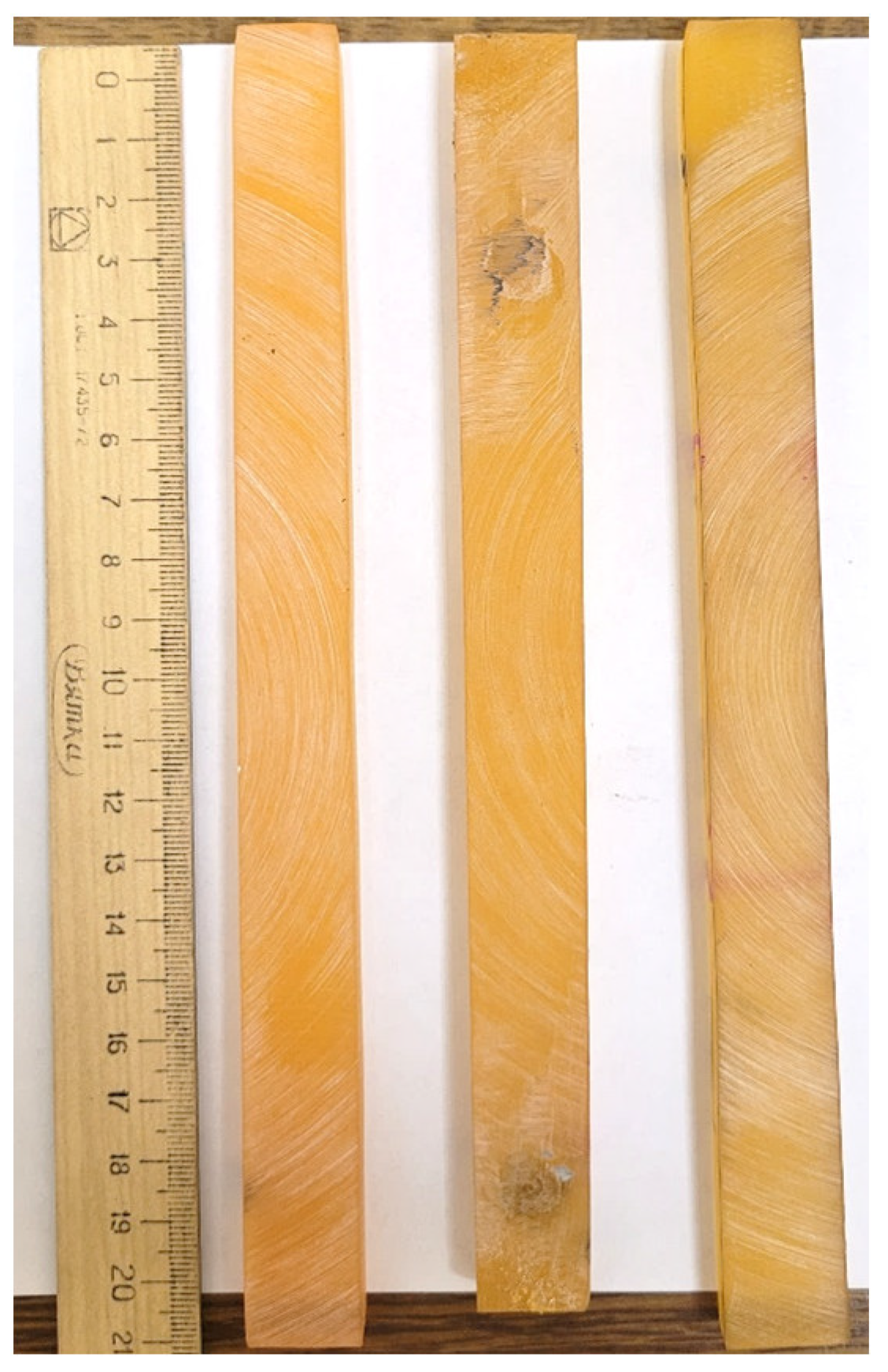
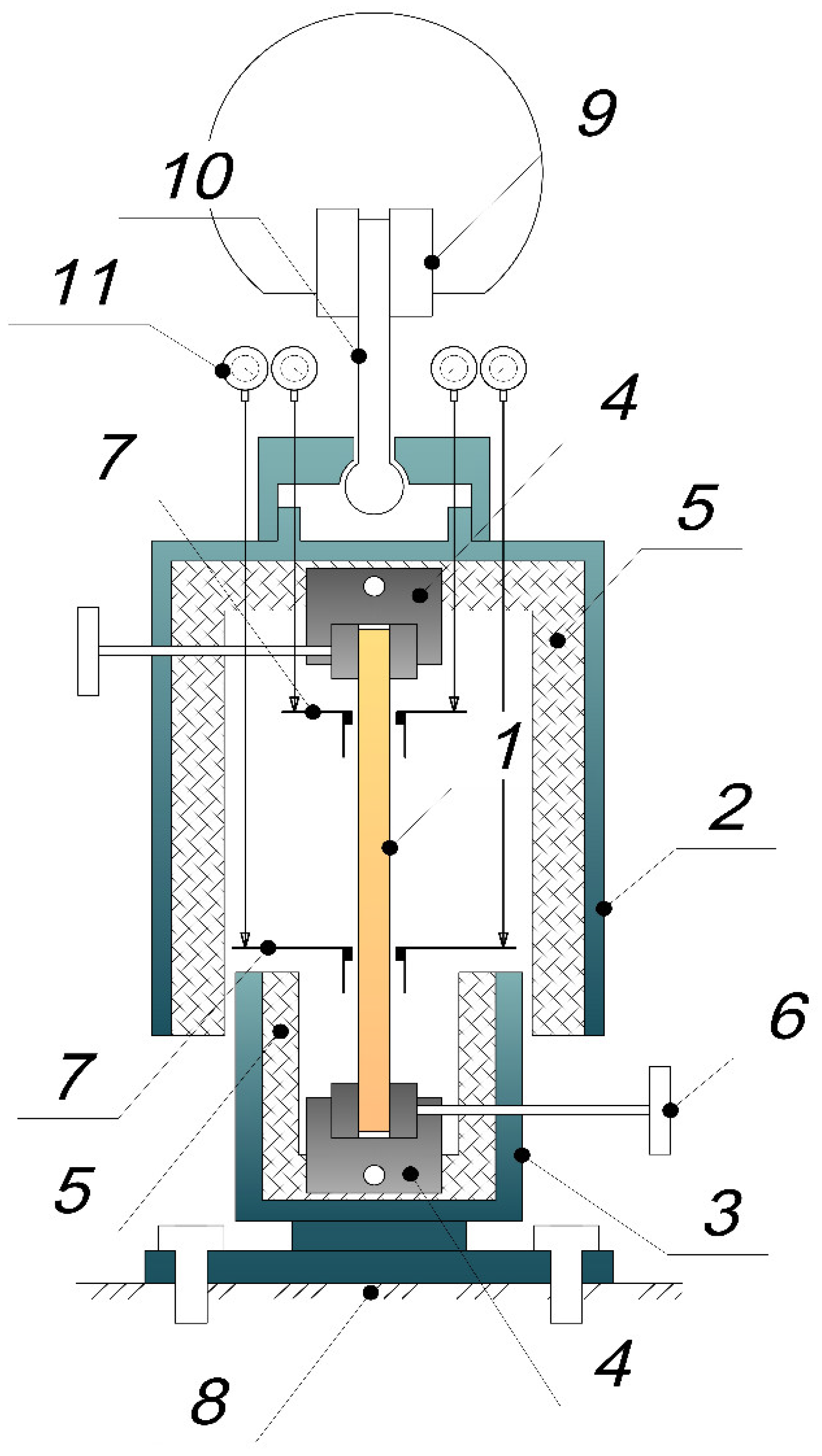
Description of the Experimental Setup
A Description of the Methodology for Determining the Mechanical Characteristics of Samples
A Description of the Methodology of the Experiment on Cyclic Thermomechanical Loading
- 5.
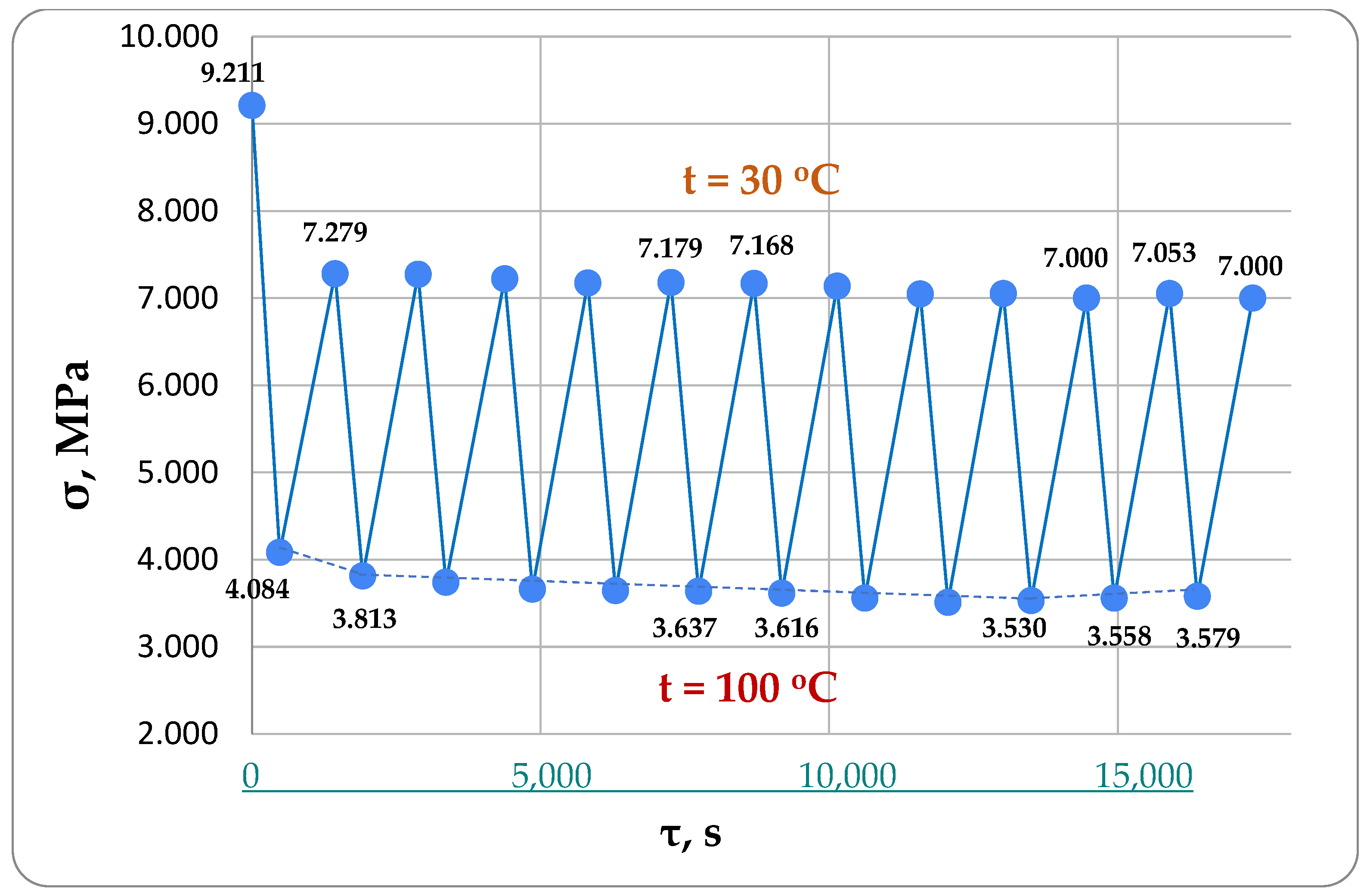
- The epoxy rod, which had angle crimps already attached, was held in place using the internal clamps from the setup described in Section A Description of the Experimental Setup. The thermal chamber and the specimen installed in it were heated to an initial constant temperature of 30 °C.
- 6.
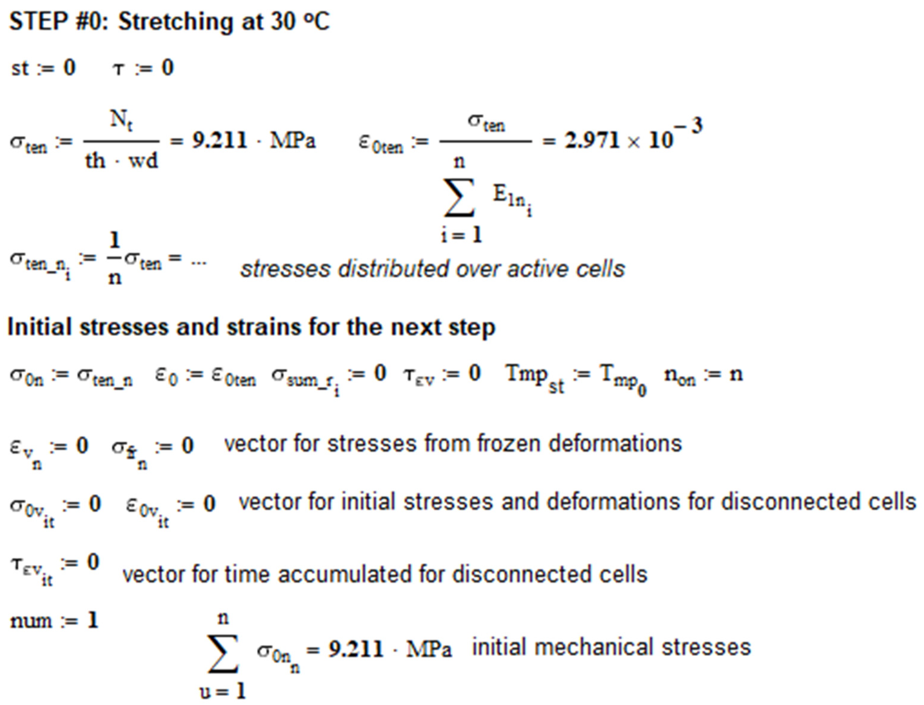
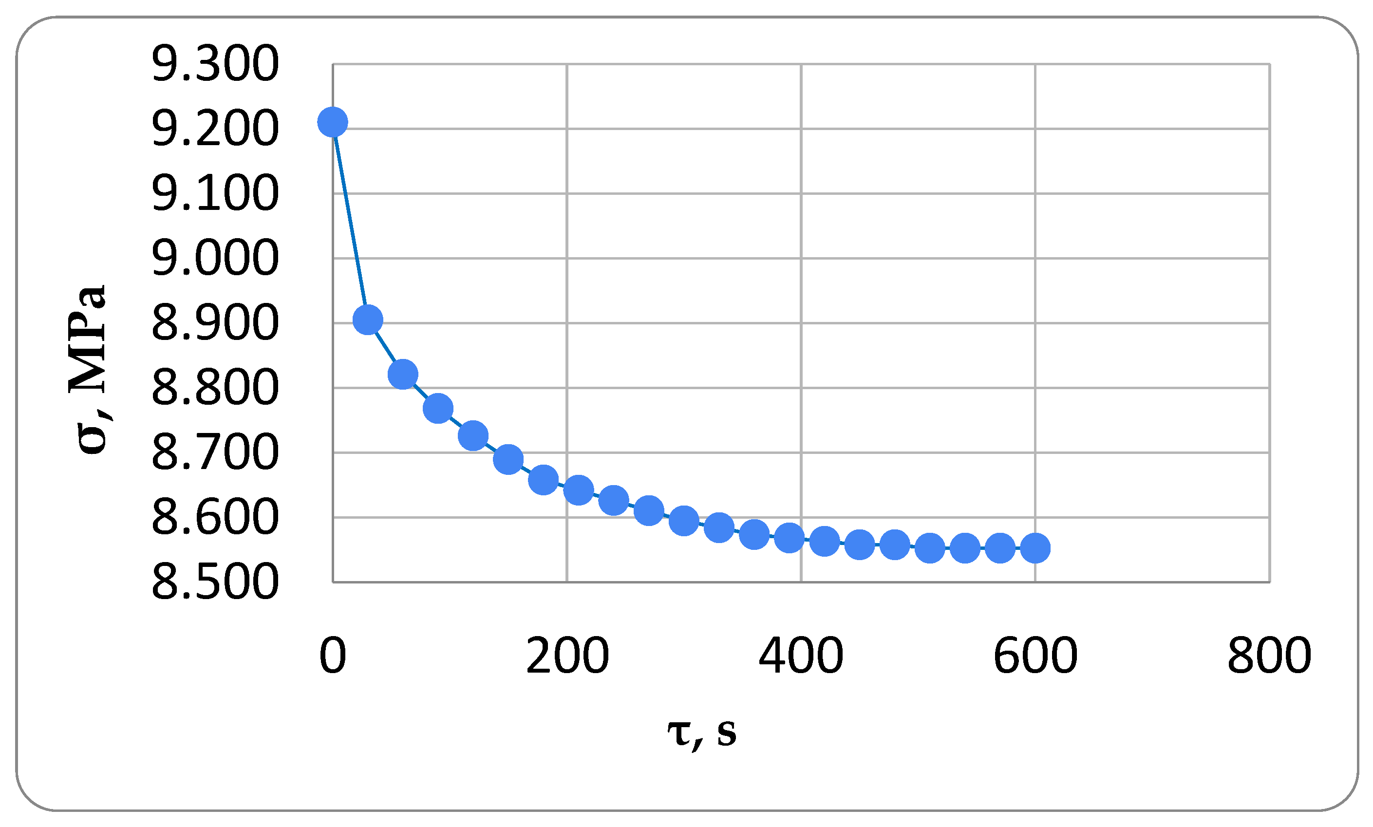
- The specimen was subjected to an initial tensile load of 1800 N (stress 9.211 MPa), and displacements were measured to determine the instantaneous modulus of elasticity E1. During the test, the clamp moved at a speed of 5 mm/min. After the load was reached, the clamps stayed in place while the load decreased due to relaxation, and the specimen’s deformation became stable.
- 7.
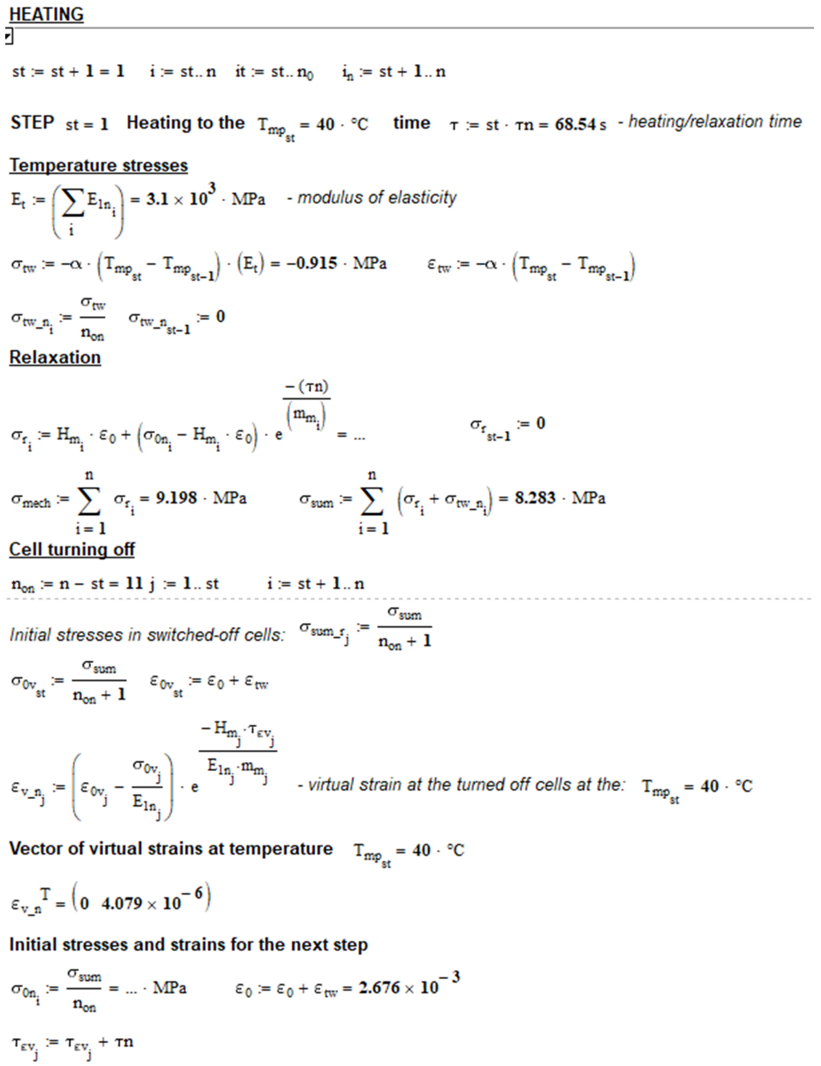
- Once the load of 1800 N was reached, the specimen’s heating mode was activated, raising its temperature to 100 °C in 8 min, achieving a heating rate of 0.1459 °C/s. As the specimen expanded under this heat, the rigid clamping caused compressive thermal stresses to build up, superimposing and reducing the tensile mechanical stresses, as shown by the stress–time curve.
- 8.
- When the temperature on the control thermocouple reached 100 °C, the sample cooling mode was activated. The sample was cooled from 100 °C to 30 °C in 16 min (cooling rate was 0.073 °C/s). Upon cooling, the specimen began to shrink, and the compressive temperature stresses that were generated during heating were reduced in the specimen.
- 9.
- The specimen went through heating and cooling cycles several times as needed. The force gauge on the testing machine recorded the load values at the peak temperature.
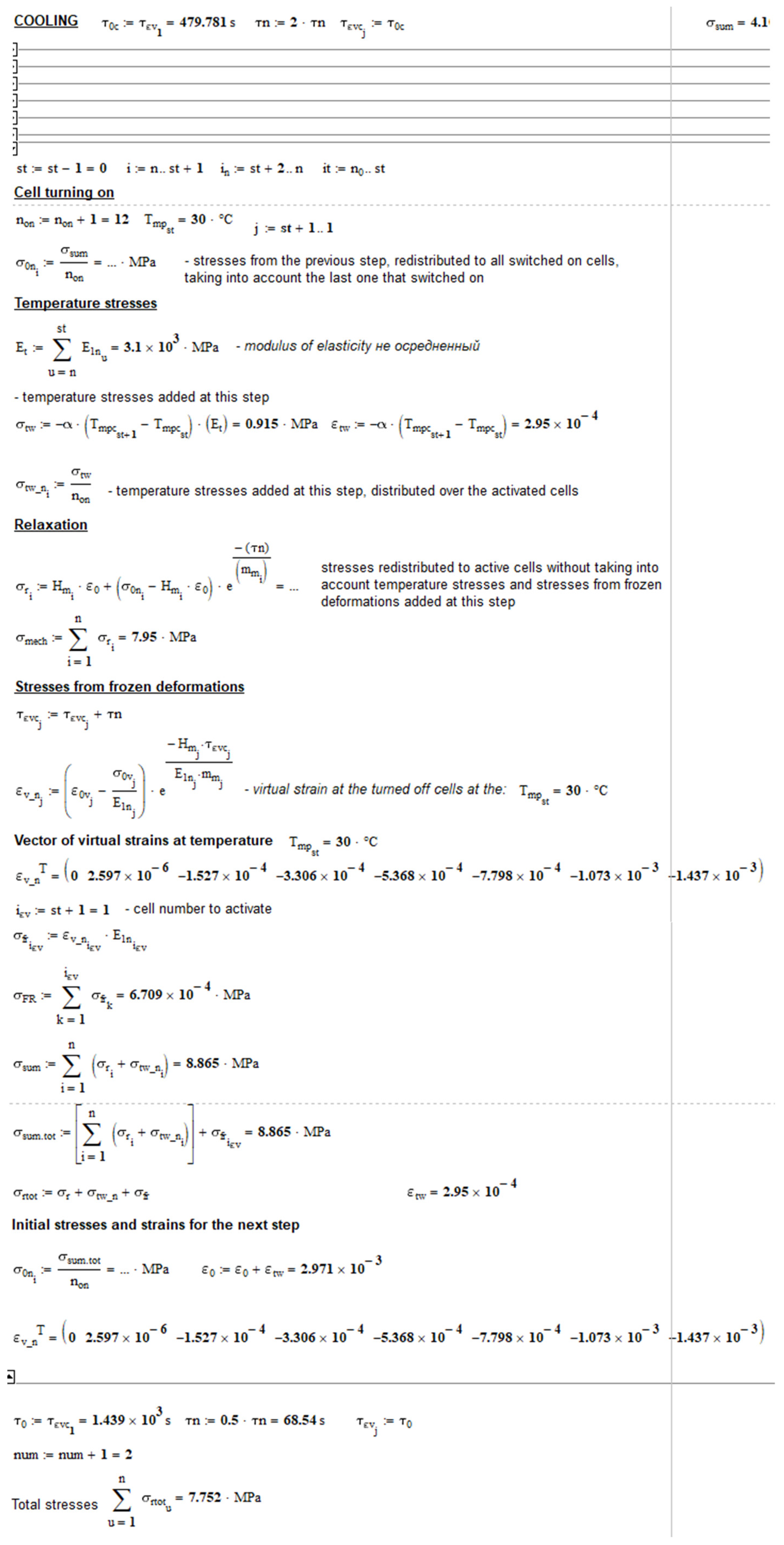
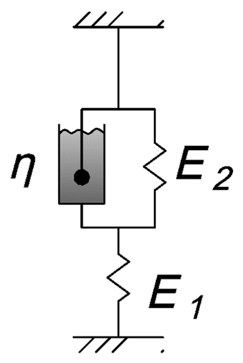
2.2.2. Methods of Theoretical Research
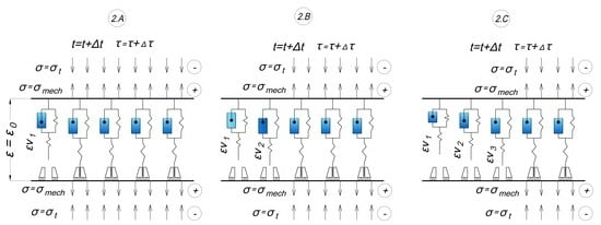
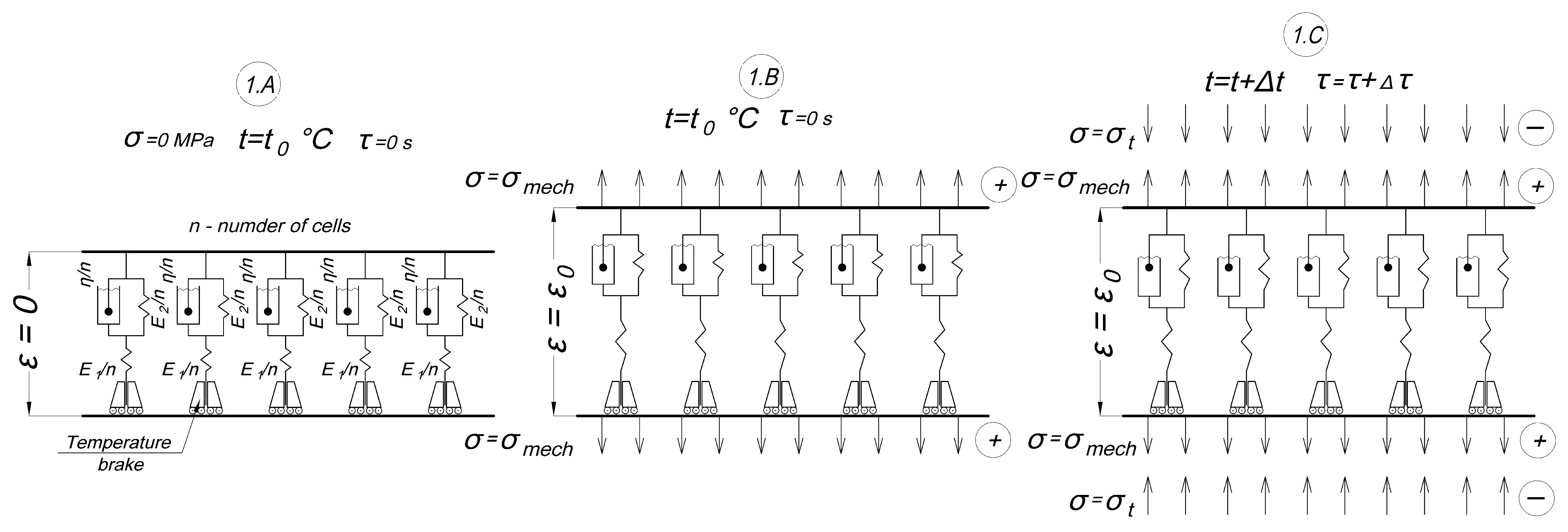
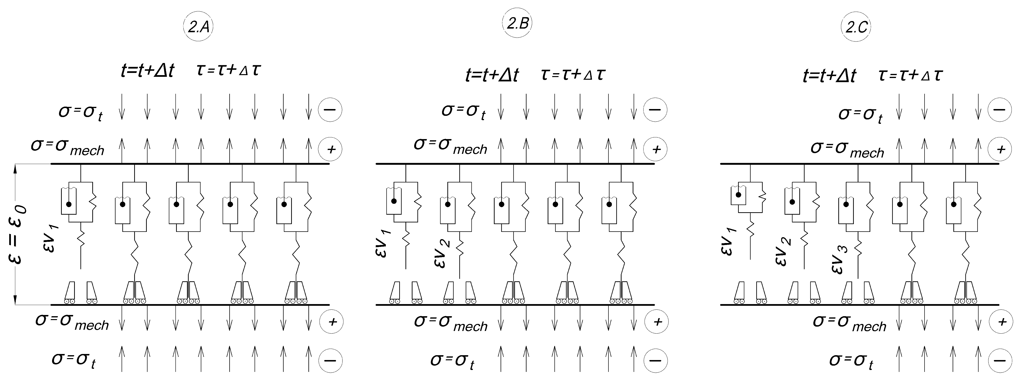
- -
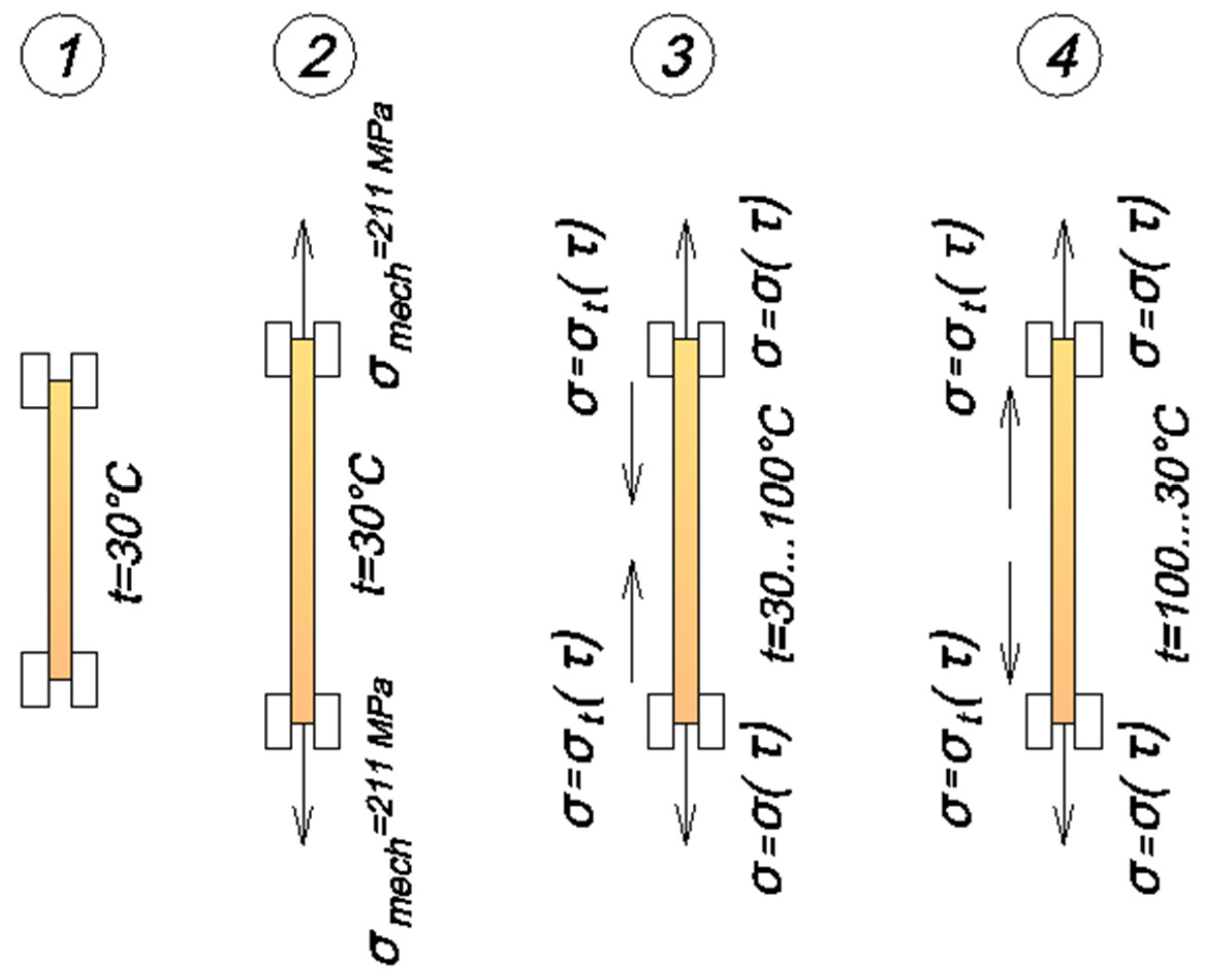
- 1.A: initial stage at zero time at initial temperature and zero stresses.
- -
- 1.B: a mechanical tensile load is applied (the time of load increase is not taken into account), mechanical stresses are evenly distributed among all cells, the strain of the specimen has increased to ε0, and the temperature is also equal to the initial one.
- -
- 1.C: heating starts, compressive thermal stresses appear, all cells are included, mechanical and thermal stresses are evenly distributed among all cells, and thermal stresses reduce mechanical stresses.
- -
- 2.A: the shutdown temperature of the first cell is reached; it is switched off and deforms according to the inverse creep law (3); before shutdown the cell was stretched, and after shutdown virtual compressive deformations grow in it.
- -
- 2.B, 2.C: the same as in 2.A but with subsequent cells; in the end there are several working cells.
- -
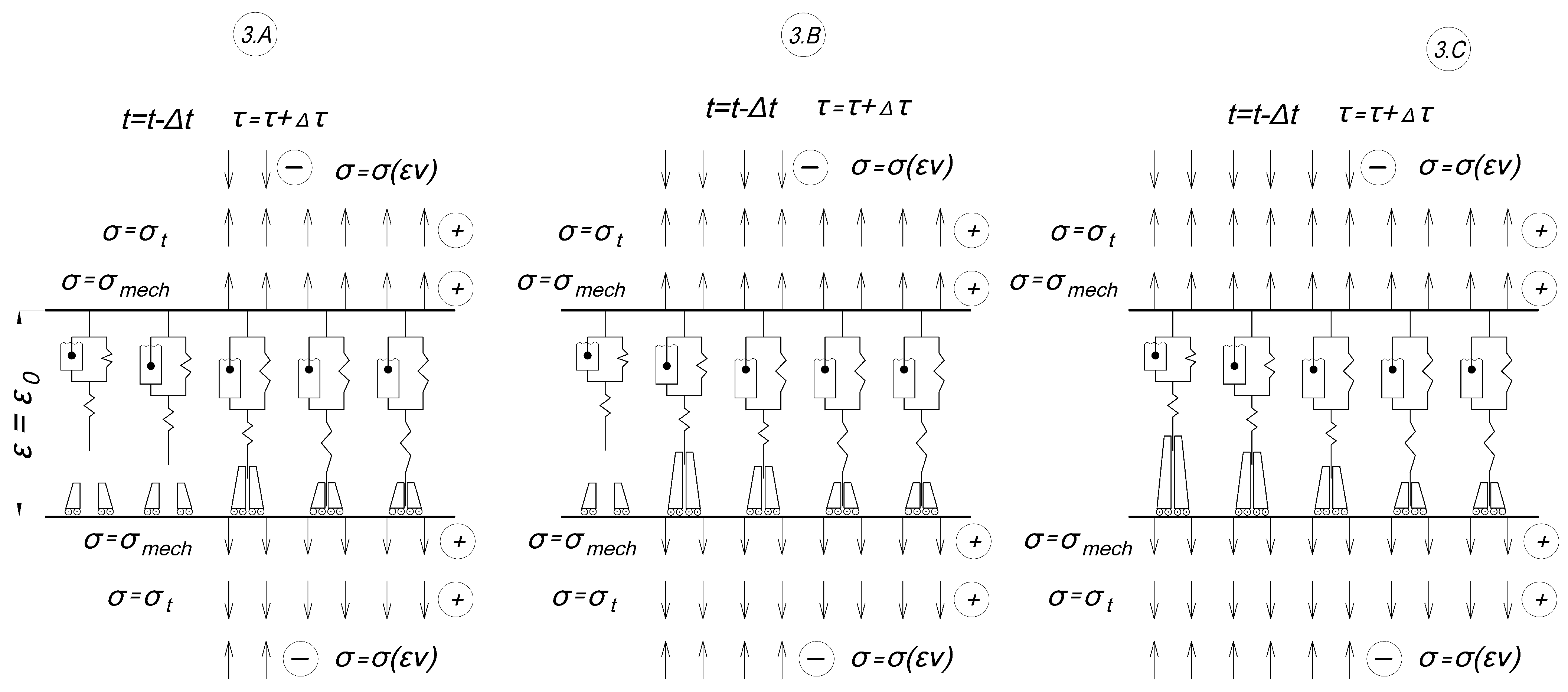
- 3.A: cooling is in progress, temperature stresses have changed sign and coincide in the direction with mechanical tensile stresses, the switching temperature of the cell that was turned off last has been reached, and then it is turned on and the strains in it turn into stresses.
- -
- 3.B, 3.C: the same as in 2.A but with subsequent cells; eventually the initial temperature is reached and all cells are turned on, with each having contributed a different value of the residual stresses at turning on.
3. Results
- -
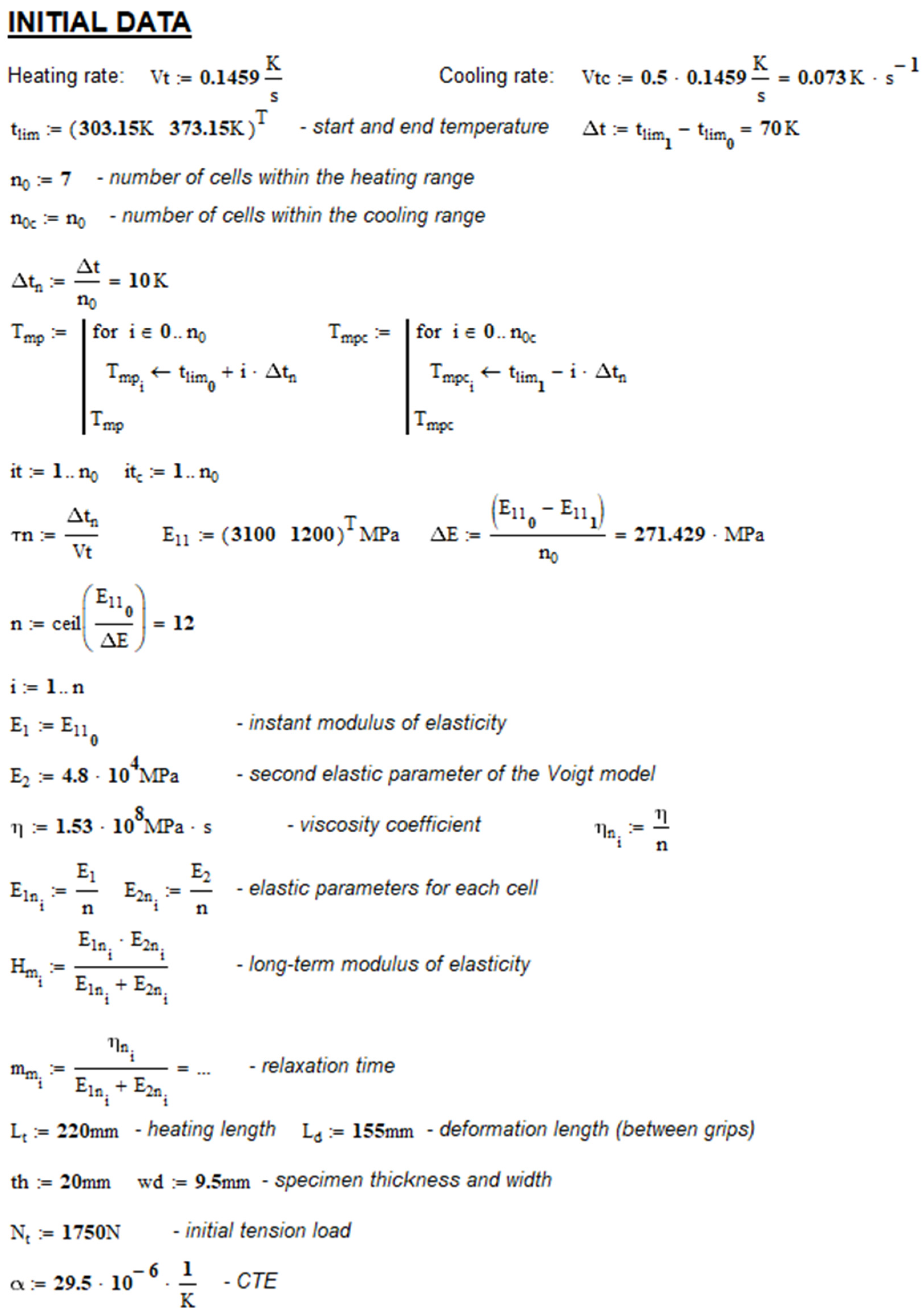
- Viscoelastic parameters at 30 °C E1 = 3100 MPa, E2 = 448,000 MPa, and η = 1.53 * 108 MPa * s.
- -
- -
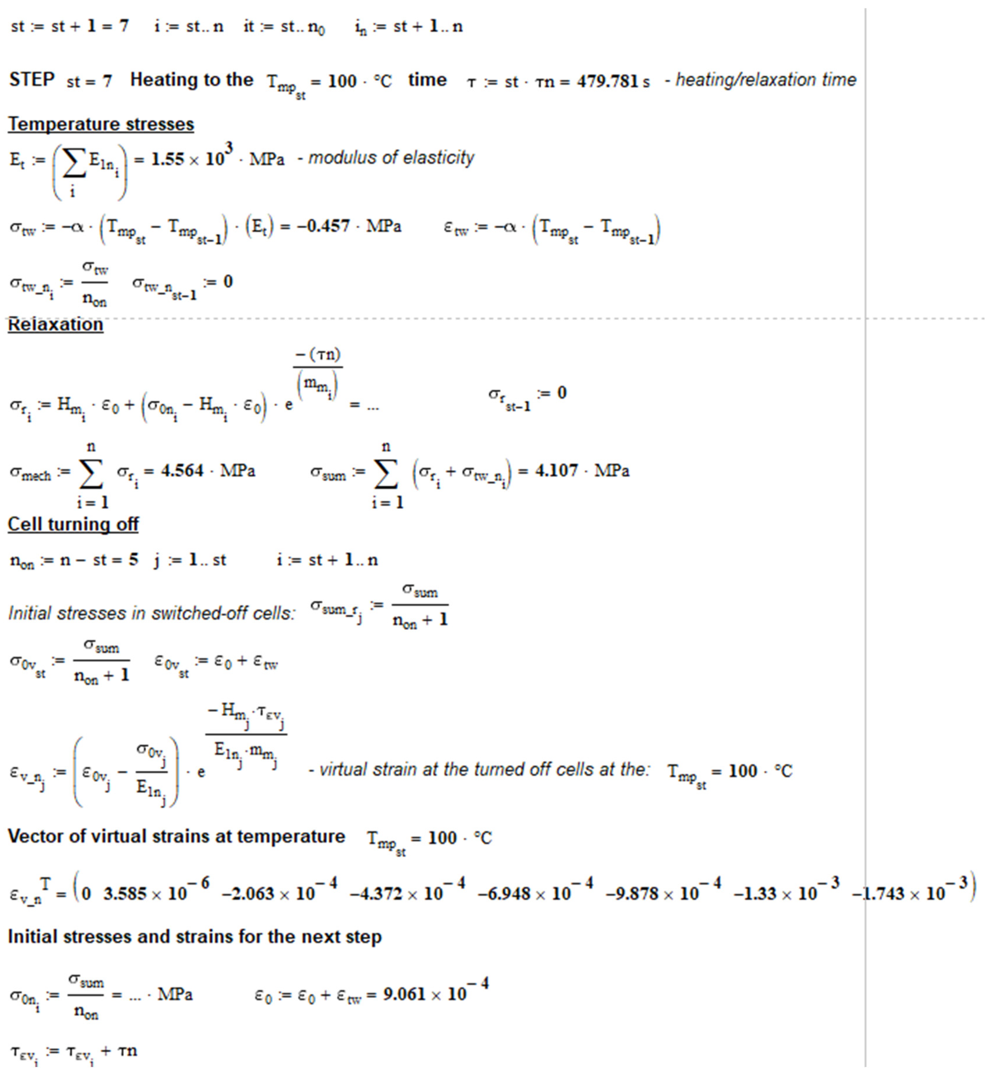
- The temperature step was taken as 10 °C.
- -
- The average coefficient of thermal expansion (CTE) was assumed to be 29.5 * 10−6 K−1 without considering its nonlinear relationship with temperature, based on previous research [45].
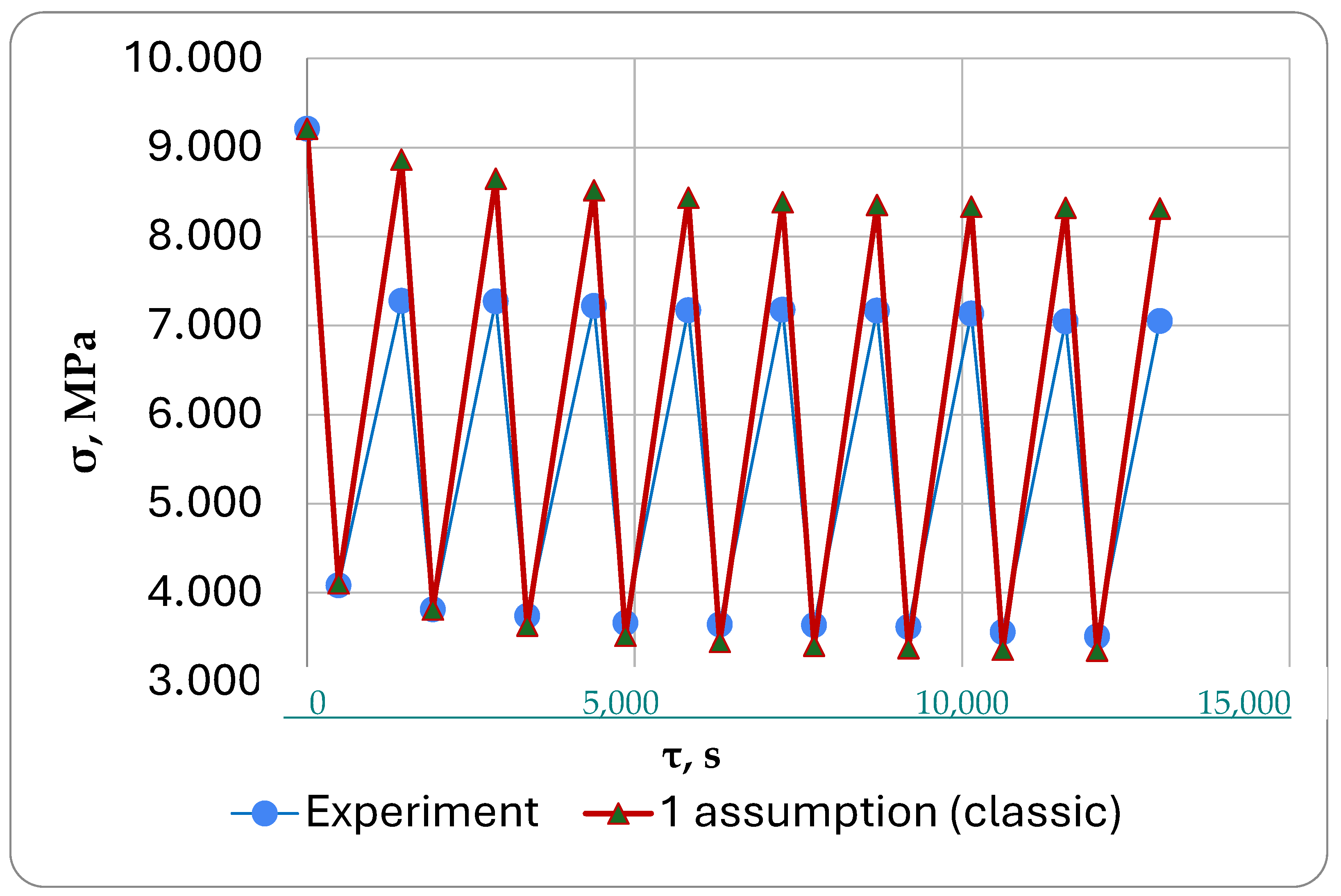
- Without considering the stresses from the cells to be turned-off (classical approach).
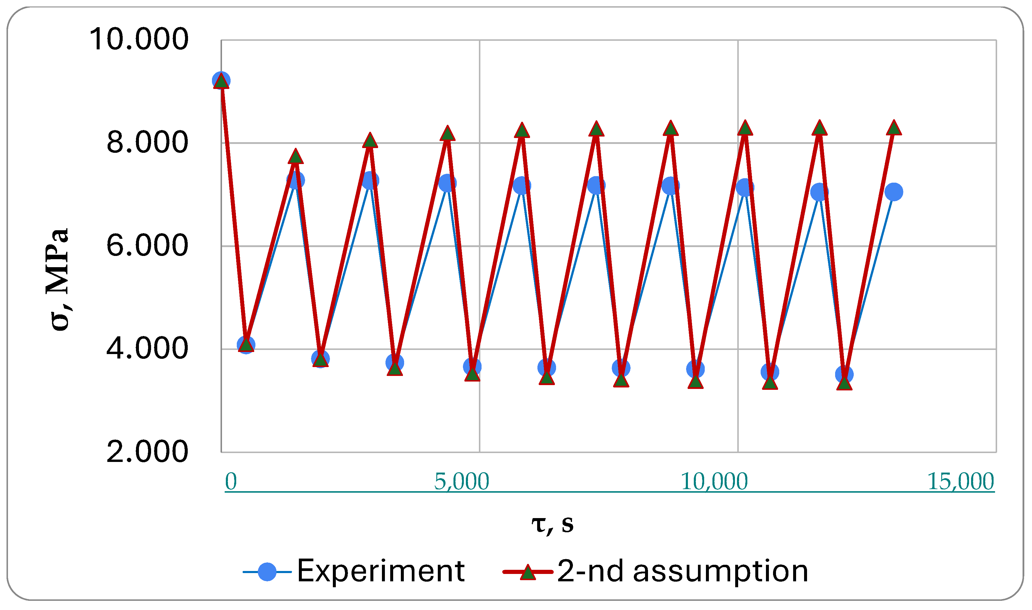
- Using the proposed multi-element model, virtual strains in the disconnected cells developed as described above according to the inverse creep law:
- 3.
- Using the proposed multi-element model, but the virtual deformations in the disconnected cells were developed without considering inverse creep (i.e., fully elastic): .
- -
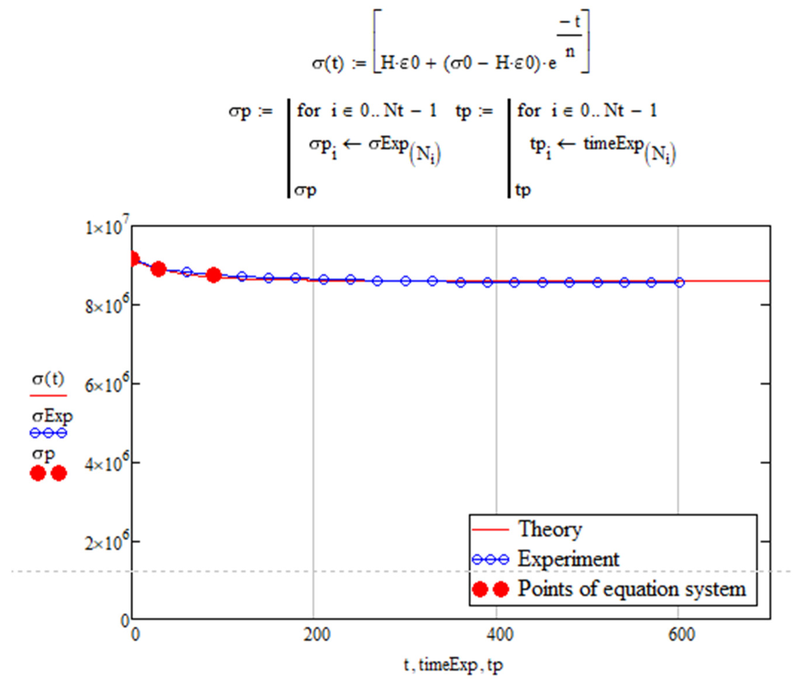
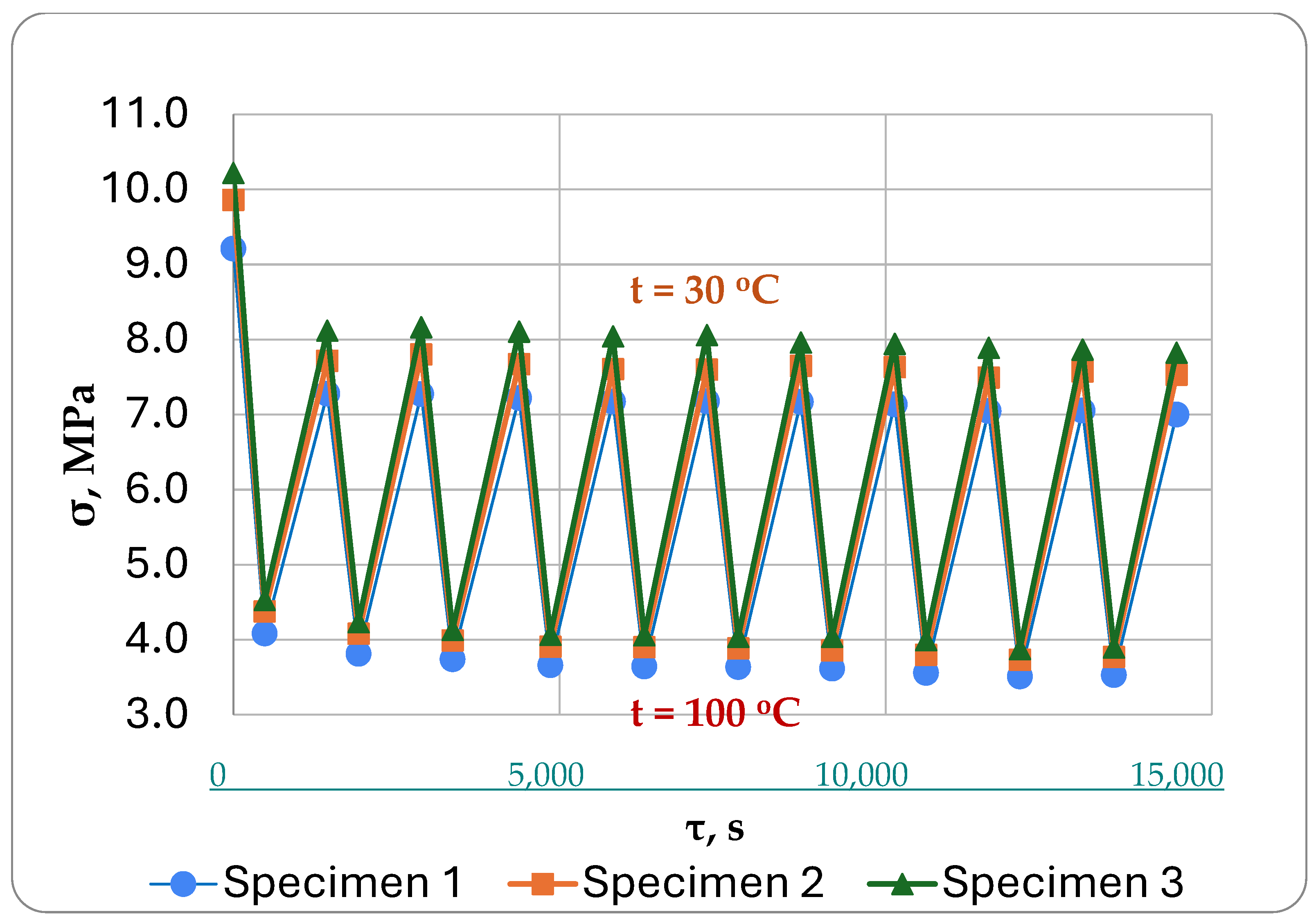
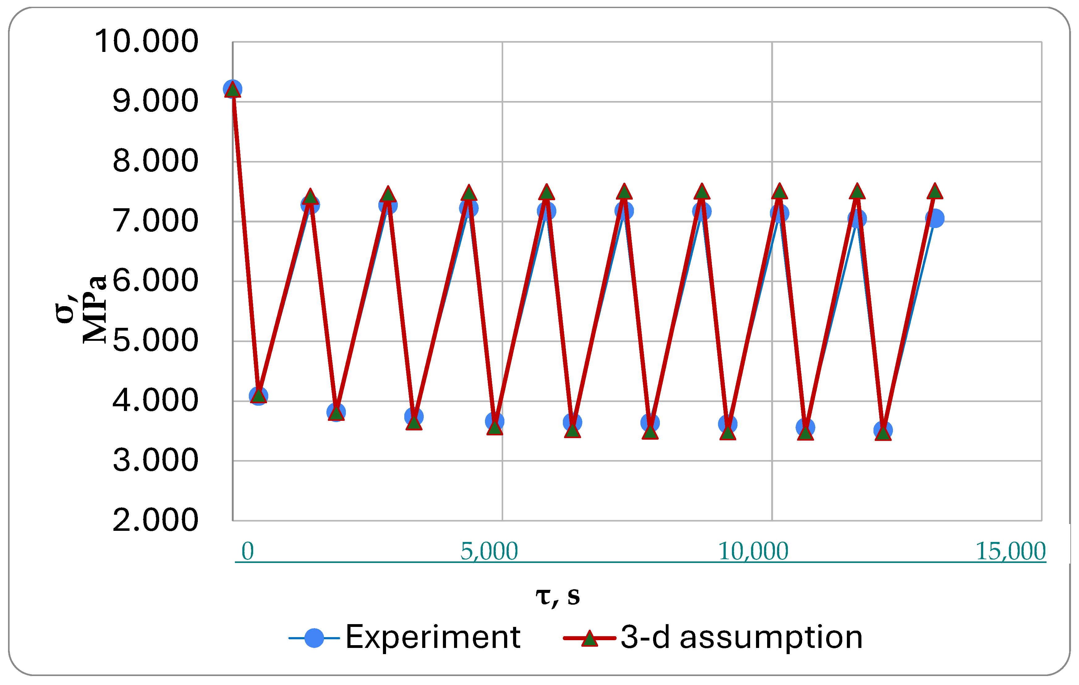
- All tested samples showed similar changes in the stress state during cyclic thermomechanical loading.
- -
- The experiment was modeled based on three different assumptions.
- -
- When comparing the modeling results with the experimental data for one of the specimens, it was observed that the simulation under the third assumption provided the closest match (with a stress difference of no more than 6%). Deformations in the switched-off cells of the model were assumed to be purely elastic, instead of following the law of inverse creep as we had first assumed.
4. Discussion
5. Conclusions
Author Contributions
Funding
Data Availability Statement
Conflicts of Interest
Appendix A

References
- McConnell, V.P. Resurgence in Corrosion-Resistant Composites. Reinf. Plast. 2005, 49, 20–25. [Google Scholar] [CrossRef]
- McConnell, V.P. Getting Ducts in a Row with Corrosion-Resistant FRP. Reinf. Plast. 2011, 55, 20–26. [Google Scholar] [CrossRef]
- Plecnik, J.M.; Gerwein, P.H.; Pham, M.G. Design and Construction of World’s Tallest Free-Standing Fiberglass Stack. Civ. Eng. 1981, 51, 57–59. [Google Scholar]
- Ding, A.X.; Ni, A.Q.; Wang, J.H. Analysis of FRP Chimneys Liners under Wind and Seismic Load. Adv. Mater. Res. 2013, 790, 193–197. [Google Scholar] [CrossRef]
- Ding, A.; Wang, J.; Ni, A. The Selection of Safety Factor of FRP Chimney for Coal-Fired Units. Fuhe Cailiao Xuebao/Acta Mater. Compos. Sin. 2013, 30, 236–239. [Google Scholar]
- Makarov, V.G.; Sinelnikova, R.M. Application of Composites in the Sulfur Acid Production. In Annual Technical Conference—ANTEC, Conference Proceedings; Society of Plastics Engineers (SPE): Mumbai, India, 2007. [Google Scholar]
- Honga, S.J.; Honga, S.H.; Doh, J.M. Materials for Flue Gas Desulfurization Systems Operating in Korea and Their Failures. Mater. High Temp. 2007, 24, 289–293. [Google Scholar] [CrossRef]
- Makarov, V.G.; Sinelnikova, R.M. Sudden Failure of Final GRP Products. In Annual Technical Conference—ANTEC, Conference Proceedings; Society of Plastics Engineers (SPE): Mumbai, India, 2010. [Google Scholar]
- Arshad, Z.; Alharthi, S.S. Enhancing the Thermal Comfort of Woven Fabrics and Mechanical Properties of Fiber-Reinforced Composites Using Multiple Weave Structures. Fibers 2023, 11, 73. [Google Scholar] [CrossRef]
- Shoaib, M.; Latif, Z.; Ali, M.; Al-Ghamdi, A.; Arshad, Z.; Wageh, S. Room Temperature Synthesized TiO2 Nanoparticles for Two-Folds Enhanced Mechanical Properties of Unsaturated Polyester. Polymers 2023, 15, 934. [Google Scholar] [CrossRef]
- Ismail, H.; Sapuan, S.M.; Ilyas, R.A. Mineral-Filled Polymer Composites Handbook, Two-Volume Set; CRC Press: Boca Raton, FL, USA, 2022. [Google Scholar]
- Rajak, D.; Pagar, D.; Menezes, P.; Linul, E. Fiber-Reinforced Polymer Composites: Manufacturing, Properties, and Applications. Polymers 2019, 11, 1667. [Google Scholar] [CrossRef]
- Bajracharya, R.M.; Manalo, A.C.; Karunasena, W.; Lau, K.T. Durability Characteristics and Property Prediction of Glass Fibre Reinforced Mixed Plastics Composites. Compos. B Eng. 2017, 116, 16–29. [Google Scholar] [CrossRef]
- Hajiloo, H.; Green, M.F.; Gales, J. Mechanical Properties of GFRP Reinforcing Bars at High Temperatures. Constr. Build. Mater. 2018, 162, 142–154. [Google Scholar] [CrossRef]
- Rami Hamad, J.A.; Megat Johari, M.A.; Haddad, R.H. Mechanical Properties and Bond Characteristics of Different Fiber Reinforced Polymer Rebars at Elevated Temperatures. Constr. Build. Mater. 2017, 142, 521–535. [Google Scholar] [CrossRef]
- Shokrieh, M.M. Residual Stresses in Composite Materials; Woodhead Publishing: Sawston, UK, 2014; Available online: https://structures.dhu.edu.cn/_upload/article/files/f6/62/f5c6159f4c86ae7a86fbd6b48811/52671c71-4c4e-41b1-a561-a9b523be64d8.pdf (accessed on 20 March 2024).
- Thakkar, B. Influence of Residual Stresses on Mechanical Behavior of Polymers. In Plastics Products Design Handbook; CRC Press: Boca Raton, FL, USA, 2020. [Google Scholar] [CrossRef]
- Shokrieh, M.M.; Safarabadi, M. Understanding Residual Stresses in Polymer Matrix Composites. In Residual Stresses in Composite Materials; Woodhead Publishing: Sawston, UK, 2021. [Google Scholar] [CrossRef]
- Jaeger, R.; Koplin, C. Measuring and Modelling Residual Stresses in Polymer-Based Dental Composites. In Residual Stresses in Composite Materials; Woodhead Publishing: Sawston, UK, 2014. [Google Scholar] [CrossRef]
- Dai, F. Understanding Residual Stresses in Thick Polymer Composite Laminates. In Residual Stresses in Composite Materials; Woodhead Publishing: Sawston, UK, 2014. [Google Scholar] [CrossRef]
- Wang, C.C.; Yue, G.Q.; Zhang, J.Z.; Liu, J.G.; Li, J. Formation and Test Methods of the Thermo-Residual Stresses for Thermoplastic Polymer Matrix Composites. In Civil, Architecture and Environmental Engineering; CRC Press: Boca Raton, FL, USA, 2020. [Google Scholar] [CrossRef]
- Hahn, H.T. Residual Stresses in Polymer Matrix Composite Laminates. J. Compos. Mater. 1976, 10, 266–278. [Google Scholar] [CrossRef]
- Abouhamzeh, M.; Sinke, J.; Benedictus, R. Prediction Models for Distortions and Residual Stresses in Thermoset Polymer Laminates: An Overview. J. Manuf. Mater. Process. 2019, 3, 87. [Google Scholar] [CrossRef]
- Baran, I.; Cinar, K.; Ersoy, N.; Akkerman, R.; Hattel, J.H. A Review on the Mechanical Modeling of Composite Manufacturing Processes. Arch. Comput. Methods Eng. 2017, 24, 365–395. [Google Scholar] [CrossRef] [PubMed]
- Parlevliet, P.P.; Bersee, H.E.N.; Beukers, A. Residual Stresses in Thermoplastic Composites—A Study of the Literature—Part I: Formation of Residual Stresses. Compos. Part A Appl. Sci. Manuf. 2006, 37, 1847–1857. [Google Scholar] [CrossRef]
- Lee, S.M.; Schile, R.D. An Investigation of Material Variables of Epoxy Resins Controlling Transverse Cracking in Composites. J. Mater. Sci. 1982, 17, 2095–2106. [Google Scholar] [CrossRef]
- Struik, L.C.E. Orientation Effects and Cooling Stresses in Amorphous Polymers. Polym. Eng. Sci. 1978, 18, 799–811. [Google Scholar] [CrossRef]
- Di Landro, L.; Pegoraro, M. Evaluation of Residual Stresses and Adhesion in Polymer Composites. Compos. Part A Appl. Sci. Manuf. 1996, 27, 847–853. [Google Scholar] [CrossRef]
- Jain, A.; Yi, A.Y. Numerical Modeling of Viscoelastic Stress Relaxation during Glass Lens Forming Process. J. Am. Ceram. Soc. 2005, 88, 530–535. [Google Scholar] [CrossRef]
- Rzanitsyn, A.R. Theory of Creep; Stroyizdat: Moscow, Russia, 1968. [Google Scholar]
- Zhang, J.T.; Zhang, M.; Li, S.X.; Pavier, M.J.; Smith, D.J. Residual Stresses Created during Curing of a Polymer Matrix Composite Using a Viscoelastic Model. Compos. Sci. Technol. 2016, 130, 20–27. [Google Scholar] [CrossRef]
- Chen, Q.; Chen, X.; Zhai, Z.; Zhu, X.; Yang, Z. Micromechanical Modeling of Viscoplastic Behavior of Laminated Polymer Composites with Thermal Residual Stress Effect. J. Eng. Mater. Technol. Trans. ASME 2016, 138, 031005. [Google Scholar] [CrossRef]
- Yuan, Z.; Wang, Y.; Yang, G.; Tang, A.; Yang, Z.; Li, S.; Li, Y.; Song, D. Evolution of Curing Residual Stresses in Composite Using Multi-Scale Method. Compos. B Eng. 2018, 155, 49–61. [Google Scholar] [CrossRef]
- Xin, X.; Liu, L.; Liu, Y.; Leng, J. Mechanical Models, Structures, and Applications of Shape-Memory Polymers and Their Composites. Acta Mech. Solida Sin. 2019, 32, 535–565. [Google Scholar] [CrossRef]
- Turusov, R.A.; Andreevskaya, G.D. Isothermal Relaxation of Temperature Stresses in Rigid Mesh Polymers. Rep. Acad. Sci. 1979, 247, 1381–1383. [Google Scholar]
- Astashkin, V.M.; Likholetov, V.V. Residual Stress Formation in Plastic Elements of Structures during Heat Changes in Conditions of Constrained Deformation. Izv. Vuzov. Constr. Archit. 1985, 10, 128–131. [Google Scholar]
- Astashkin, V.M.; Zholudov, V.S. Chimneys and Elements of Gas-Escape Paths Made of Polymer Composites; Gusev, B.V., Ed.; GySEV: Chelyabinsk, Russia, 2011. [Google Scholar]
- Karol Argasinski, J.; Loosbergh, M.E. Halar-Lined Chimney Remains Maintenance-Free. Power. 1 December 2009. Available online: https://www.powermag.com/halar-lined-chimney-remains-maintenance-free/ (accessed on 20 March 2024).
- Zarghamee, M.S.; Brainerd, M.L.; Tigue, D.B. On Thermal Blistering of FRP Chimney Liners. J. Struct. Eng. 1986, 112, 677–691. [Google Scholar] [CrossRef]
- Mikhail, A.E.; El Damatty, A.A. Non-Linear Analysis of FRP Chimneys under Thermal and Wind Loads. Thin-Walled Struct. 1999, 35, 289–309. [Google Scholar] [CrossRef]
- Astashkin, V.M.; Tereshchuk, S.V. Methods of Description of Stressed State of Structures from Laminated Plastics under Axisymmetric Alternating Thermal Influence. In Investigations on Building Materials, Constructions and Mechanics: Collection of Scientific Works; Publisher of Chelyabisk Polythechnical University: Chelyabinsk, Russia, 1991; pp. 21–26. [Google Scholar]
- Borisenkova, E.K.; Dreval, V.E.; Vinogradov, G.V.; Kurbanaliev, M.K.; Moiseyev, V.V.; Shalganova, V.G. Transition of Polymers from the Fluid to the Forced High-Elastic and Leathery States at Temperatures above the Glass Transition Temperature. Polymer 1982, 23, 91–99. [Google Scholar] [CrossRef]
- Korolev, A.; Mishnev, M.; Vatin, N.I.; Ignatova, A. Prolonged Thermal Relaxation of the Thermosetting Polymers. Polymers 2021, 13, 4104. [Google Scholar] [CrossRef]
- Korolev, A.; Mishnev, M.; Zherebtsov, D.; Vatin, N.I.; Karelina, M. Polymers under Load and Heating Deformability: Modelling and Predicting. Polymers 2021, 13, 428. [Google Scholar] [CrossRef]
- Korolev, A.; Mishnev, M.; Ulrikh, D.V. Non-Linearity of Thermosetting Polymers’ and GRPs’ Thermal Expanding: Experimental Study and Modeling. Polymers 2022, 14, 4281. [Google Scholar] [CrossRef]


| Specimen Number | Section Width, mm | Section Thickness, mm | Length between Clamps, mm |
|---|---|---|---|
| 1 | 20.0 | 9.5 | 155 |
| 2 | 19.7 | 8.5 | 155 |
| 3 | 19.6 | 9.0 | 155 |
| Designation | Value | Unit of Measurement | Description |
|---|---|---|---|
| E1 | 3100 | MPa | Instantaneous modulus of elasticity at 30 °C |
| E1(100) | 1200 | MPa | Instantaneous modulus of elasticity at 100 °C [43,44] |
| E2 | 4.8 × 10⁴ | MPa | Elastic parameter of Kelvin–Voigt model at 30 °C |
| η | 1.53 × 10⁸ | MPa × s | Viscosity at 30 °C |
| α | 29.5 × 10⁻⁶ | 1/K | Coefficient of thermal expansion [45] |
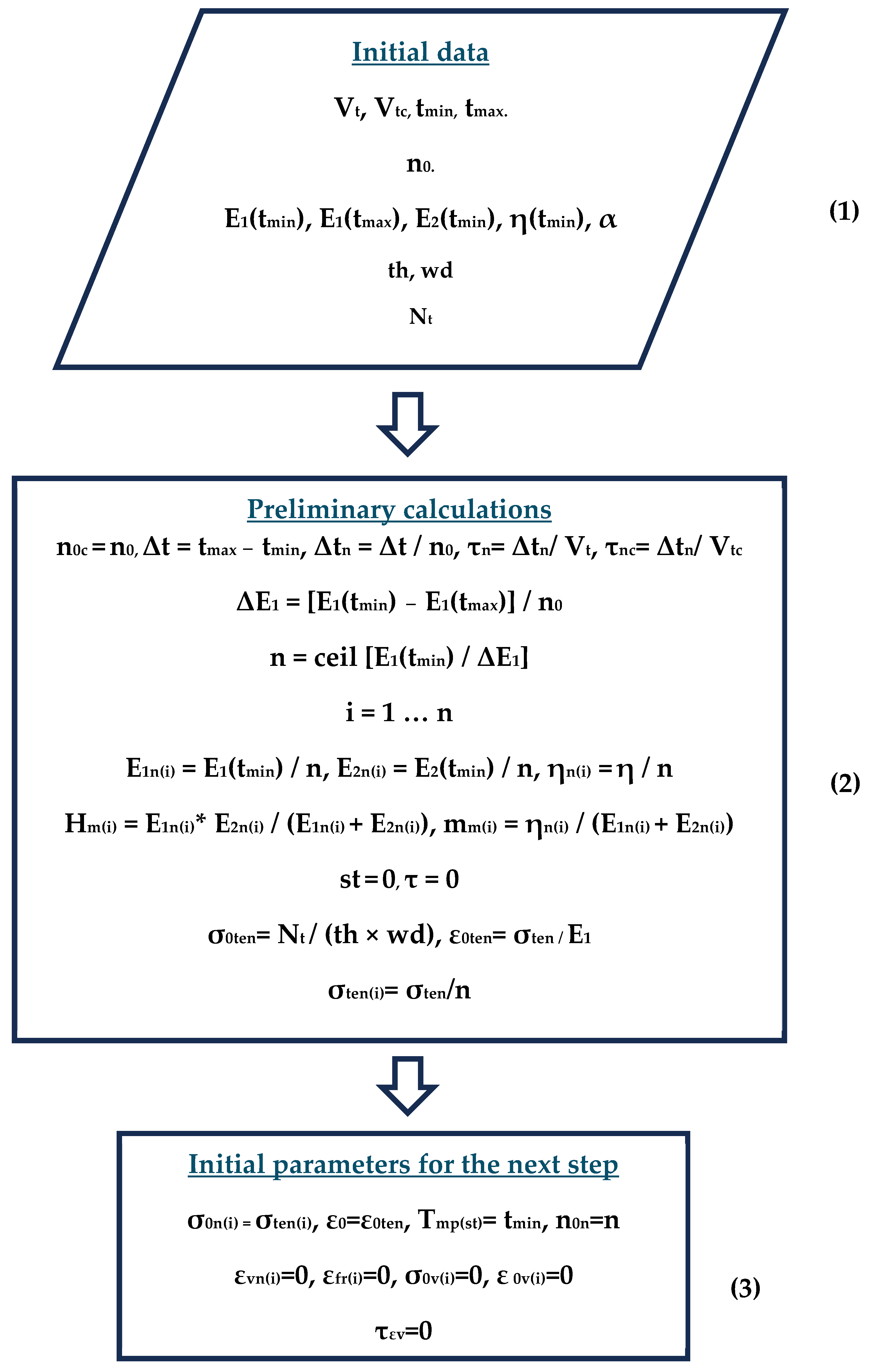
| Number Block | Description | Parameters | Parameter Description |
|---|---|---|---|
| 1 | Input of initial data | Vt, Vtc | Heating, cooling rate |
| tmin, tmax | Min. and max. heating temperatures | ||
| n0 | Number of cells within the heating range | ||
| E1(tmin), E1(tmax), E2(tmin), η(tmin), α | Instantaneous elastic modulus at minimum and maximum temperature, Kelvin–Voigt model elastic parameter and viscosity at minimum temperature, coefficient of thermal expansion | ||
| th, wd | Sample thickness and width | ||
| Nt | Tensile force on the sample | ||
| 2 | Preliminary calculations | ΔE1 | Instantaneous modulus of elasticity corresponding to one cell of the model |
| n | Total number of cells | ||
| E1n(i), E2n(i), ηn(i), Hm(i), mm(i) | Mechanical parameters corresponding to the i-th cell of the model (the entry i = 1 …n means that the counter i varies from 1 to n with step 1). As a result, vectors E1n, E2n, ηn, Hm, and mm containing i elements are formed | ||
| st, τ | Calculation step and its corresponding time | ||
| σ0ten, ε0ten | Initial tensile stress and strain | ||
| σten(i) | Initial tensile stress absorbed by one cell | ||
| 3 | Initial parameters for the next calculation step | Tmp(st) | Temperature corresponding to step st |
| n0n | Total number of included cells | ||
| σ0n(i), ε0, εvn(i), εfr(i), σ0v(i), ε0v(i), τεv | Initial vectors and parameters for the next calculation step |
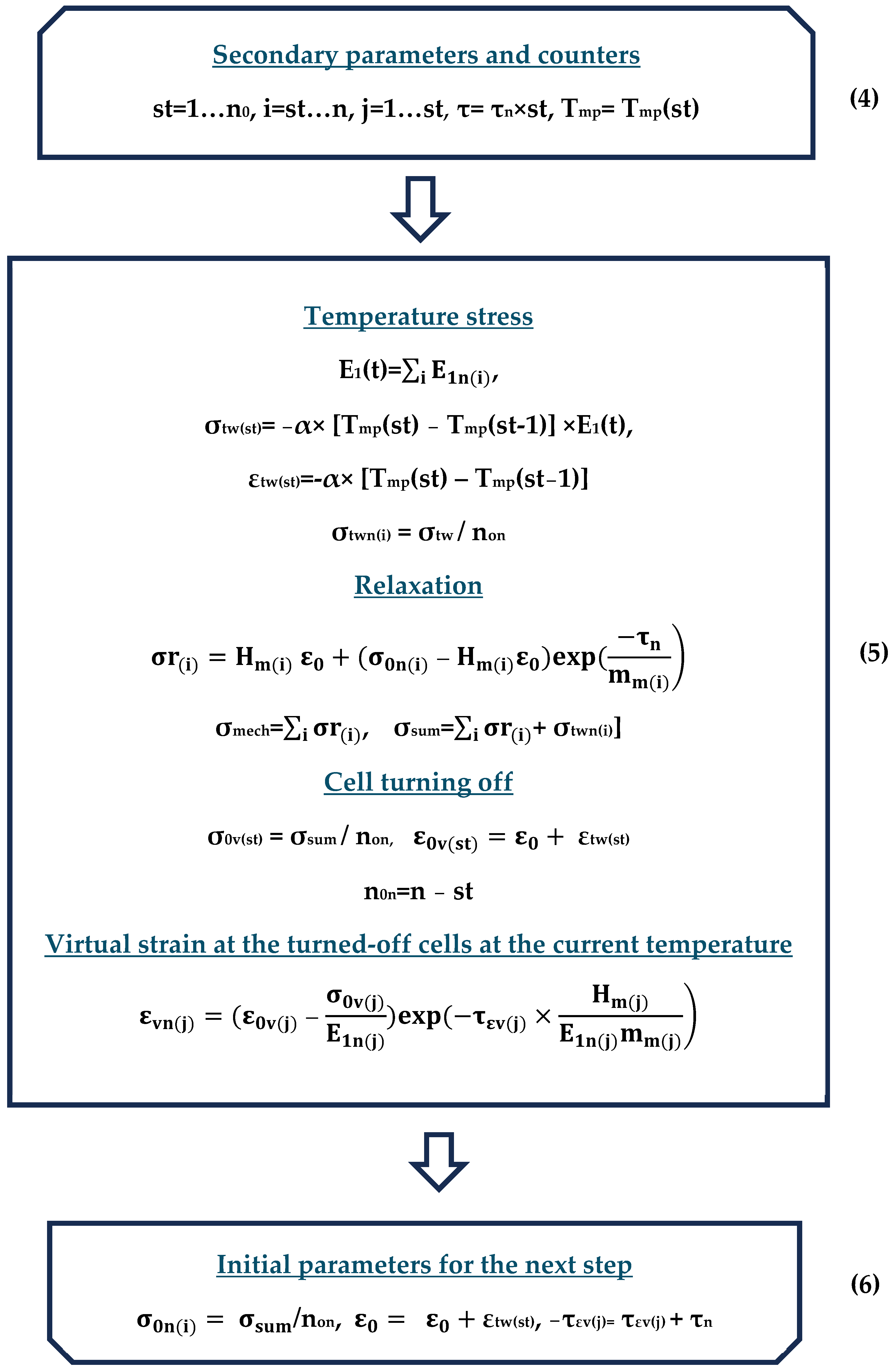
| Number Block | Description | Parameters | Parameter Description |
|---|---|---|---|
| 4 | Start of the heating cycle at the current step | St, i, j, τ, Tmp | Secondary parameters and counters |
| 5 | Basic calculations in the heating cycle | E1(t) | Instantaneous modulus of elasticity corresponding to temperature t |
| σtw(st), εtw(st) | Temperature stresses and strains at step st | ||
| σtwn(i) | Temperature stresses in the i-th switched-on cell | ||
| σr(i) | Stresses in the i-th cell after relaxation for time increment τn | ||
| σ0sum | Total (mechanical + temperature) stresses summed over all working cells | ||
| σ0v(st), ε0v(st) | Initial stresses and strains for calculating virtual strains at step st | ||
| n0n = n − st | Number of enabled cells at step st | ||
| Virtual strains in the j-th disconnected cell at the current step | |||
| 6 | End of heating cycle at current step | σ0n(i), ε0, τεv(j) | Initial parameters for the next calculation step |
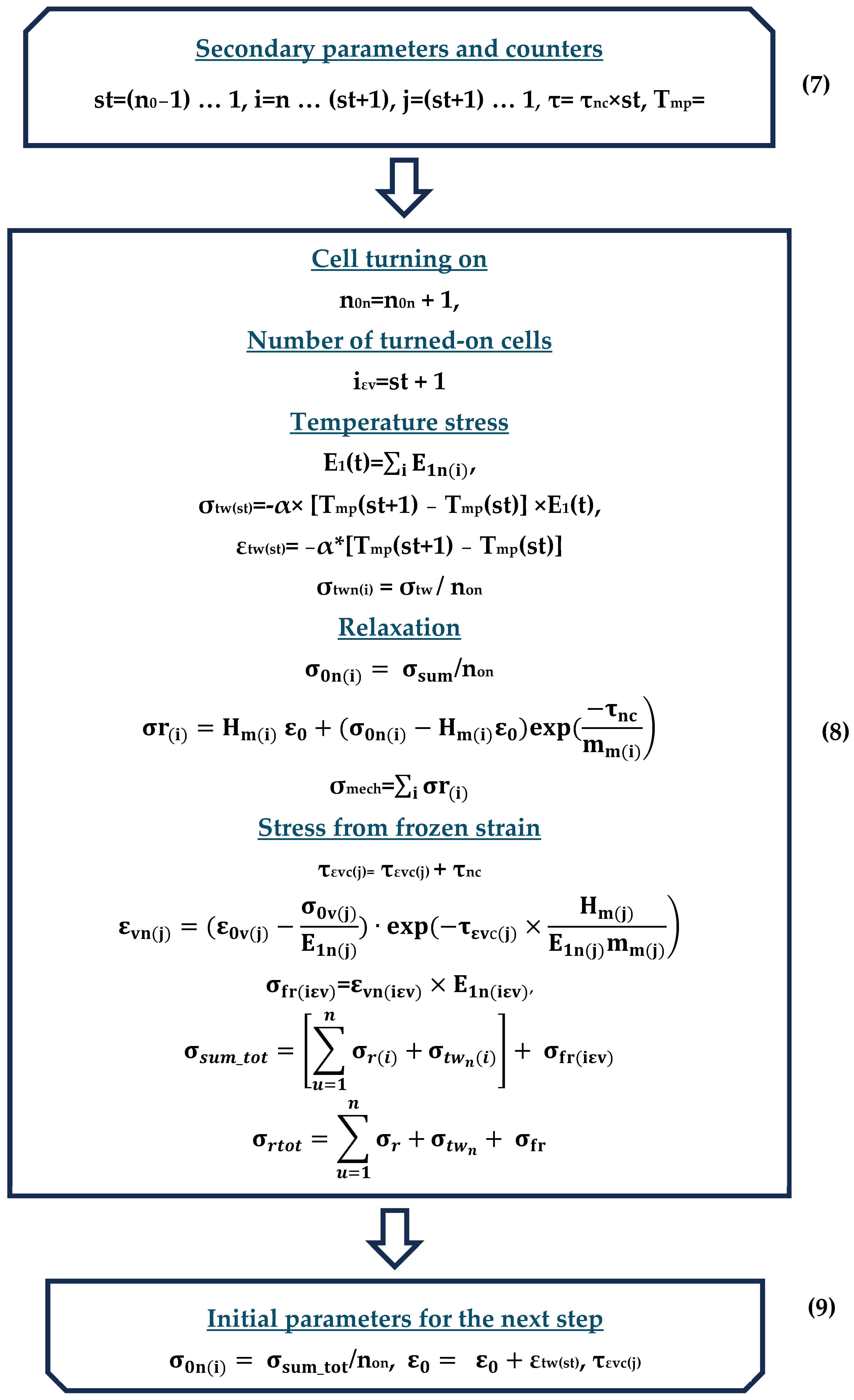
| Number Block | Description | Parameters | Parameter Description |
|---|---|---|---|
| 7 | Start of the cooling cycle in the current step | St, i, j, τ, Tmp | Secondary parameters and counters |
| 8 | Basic calculations in the cooling cycle | n0n | Number of enabled cells in the current step |
| E1(t) | Instantaneous modulus of elasticity corresponding to temperature t | ||
| σtw(st), εtw(st) | Temperature stresses and deformations at step st | ||
| σtwn(i) | Temperature stresses in the i-th switched-on cell | ||
| σr(i) | Stresses in the i-th cell after relaxation for time increment τnc | ||
| σ0mech | Stresses summarized over all working cells | ||
| Virtual deformations in the j-th disconnected cell at the current step | |||
| The stresses resulting from virtual deformations in the cell at the moment of its activation after being cooled to the temperature corresponding to the current calculation step | |||
| Total stresses (including addition of stresses from virtual deformations in the cell keyed at the current step) | |||
| Total stresses in all cells | |||
| 9 | End of the cooling cycle in the current step | σ0n(i), ε0, τεvc(j) | Initial parameters for the next calculation step |
Disclaimer/Publisher’s Note: The statements, opinions and data contained in all publications are solely those of the individual author(s) and contributor(s) and not of MDPI and/or the editor(s). MDPI and/or the editor(s) disclaim responsibility for any injury to people or property resulting from any ideas, methods, instructions or products referred to in the content. |
© 2024 by the authors. Licensee MDPI, Basel, Switzerland. This article is an open access article distributed under the terms and conditions of the Creative Commons Attribution (CC BY) license (https://creativecommons.org/licenses/by/4.0/).
Share and Cite
Mishnev, M.; Korolev, A.; Zadorin, A.; Astashkin, V. Cyclic Thermomechanical Loading of Epoxy Polymer: Modeling with Consideration of Stress Accumulation and Experimental Verification. Polymers 2024, 16, 910. https://doi.org/10.3390/polym16070910
Mishnev M, Korolev A, Zadorin A, Astashkin V. Cyclic Thermomechanical Loading of Epoxy Polymer: Modeling with Consideration of Stress Accumulation and Experimental Verification. Polymers. 2024; 16(7):910. https://doi.org/10.3390/polym16070910
Chicago/Turabian StyleMishnev, Maxim, Alexander Korolev, Alexander Zadorin, and Vladimir Astashkin. 2024. "Cyclic Thermomechanical Loading of Epoxy Polymer: Modeling with Consideration of Stress Accumulation and Experimental Verification" Polymers 16, no. 7: 910. https://doi.org/10.3390/polym16070910
APA StyleMishnev, M., Korolev, A., Zadorin, A., & Astashkin, V. (2024). Cyclic Thermomechanical Loading of Epoxy Polymer: Modeling with Consideration of Stress Accumulation and Experimental Verification. Polymers, 16(7), 910. https://doi.org/10.3390/polym16070910