

Modeling Approach for Reactive Injection Molding of Polydisperse Suspensions with Recycled Thermoset Composites


Abstract
:1. Introduction
2. Experimental Setup
3. Process and Material Modeling
3.1. Governing Equations
3.2. Constitutive Material Models
3.2.1. Extension of the Reactive Viscosity Model for Polydisperse Suspensions
3.2.2. Reaction Kinetics Model
4. Mold-Filling Simulation in OpenFOAM
5. Results and Discussion
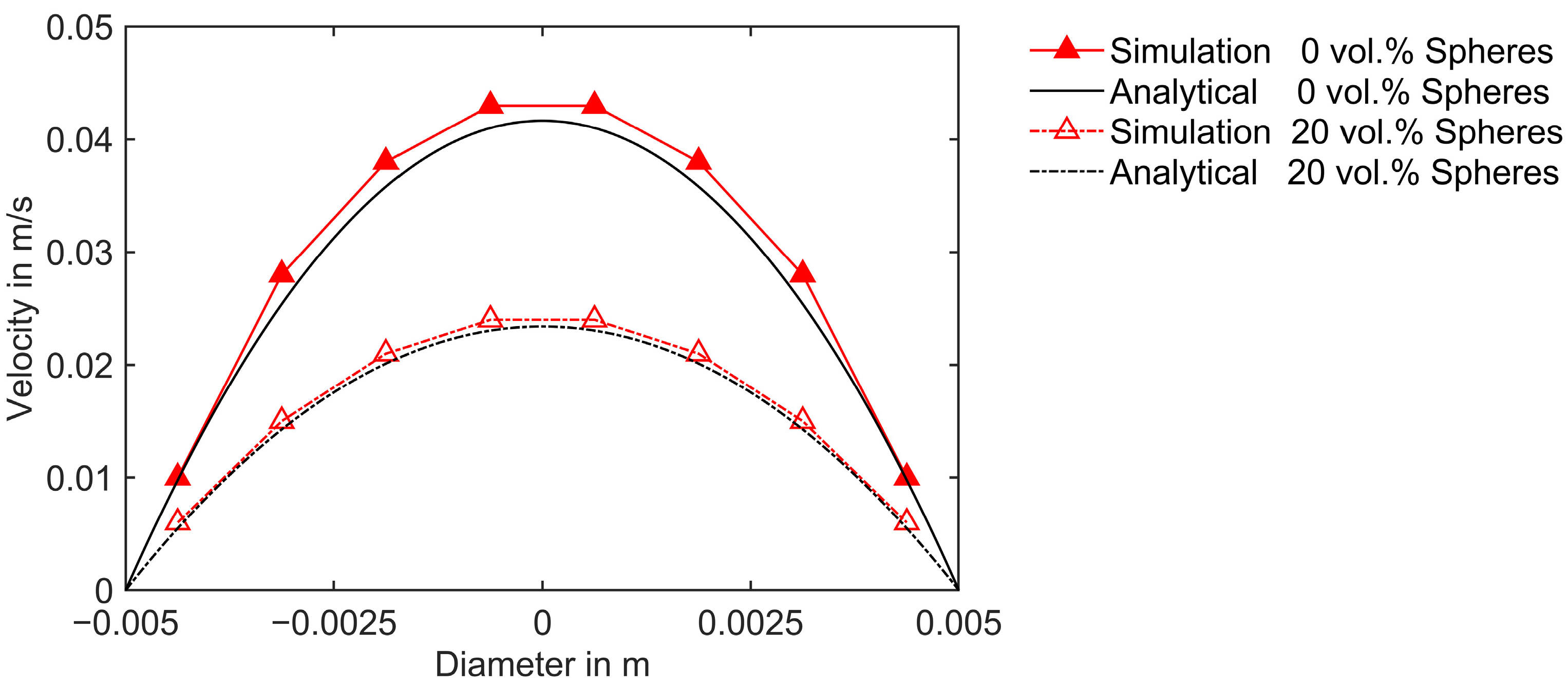
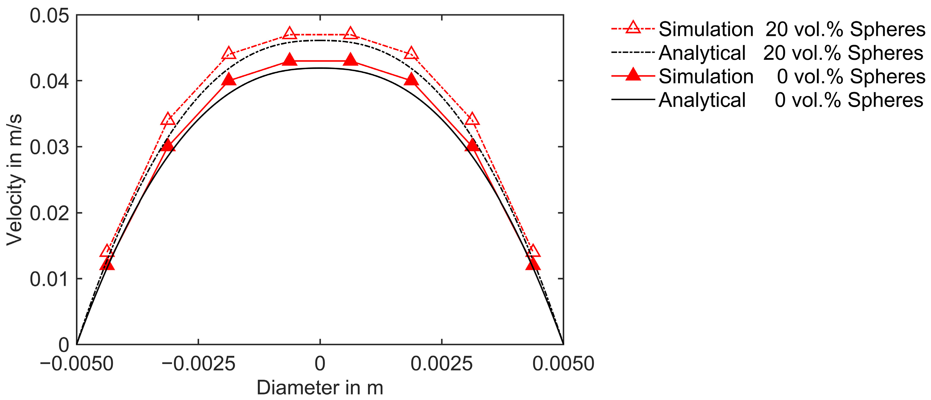
5.1. Numerical Verification
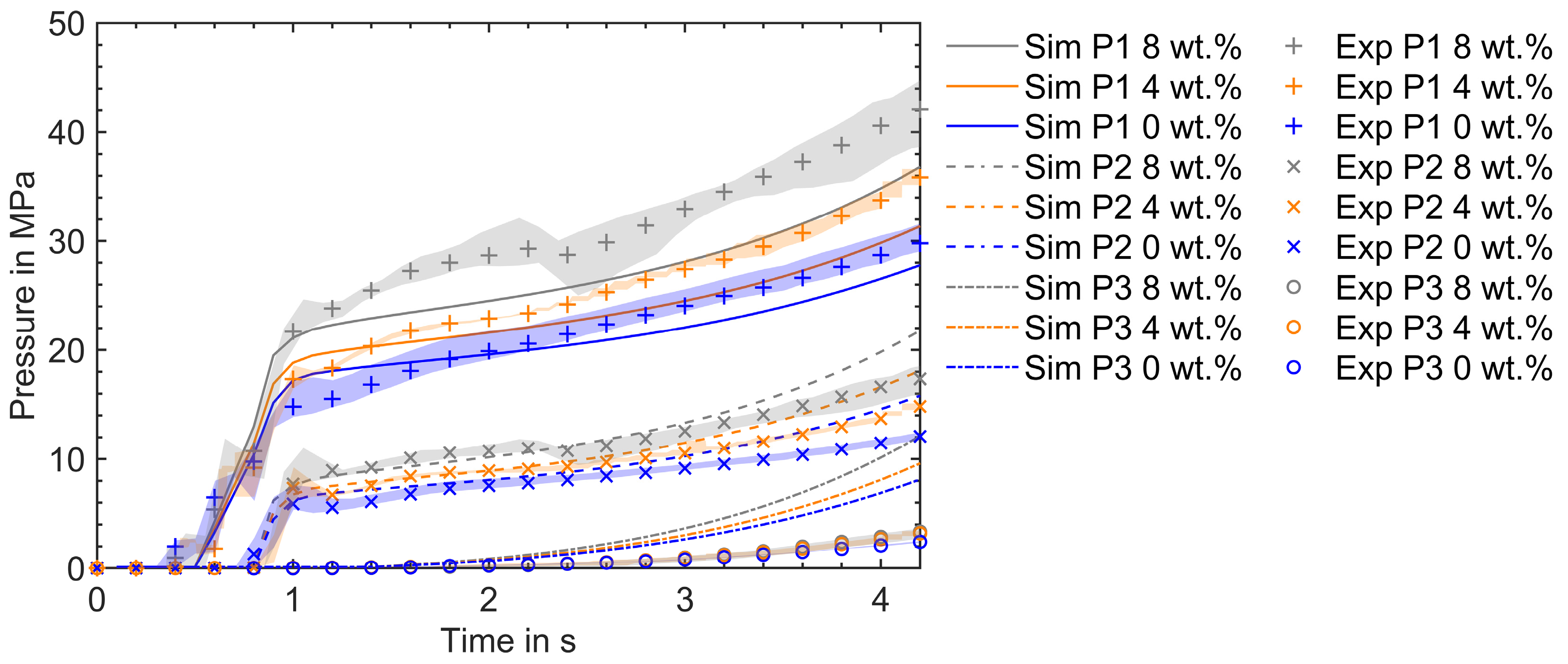
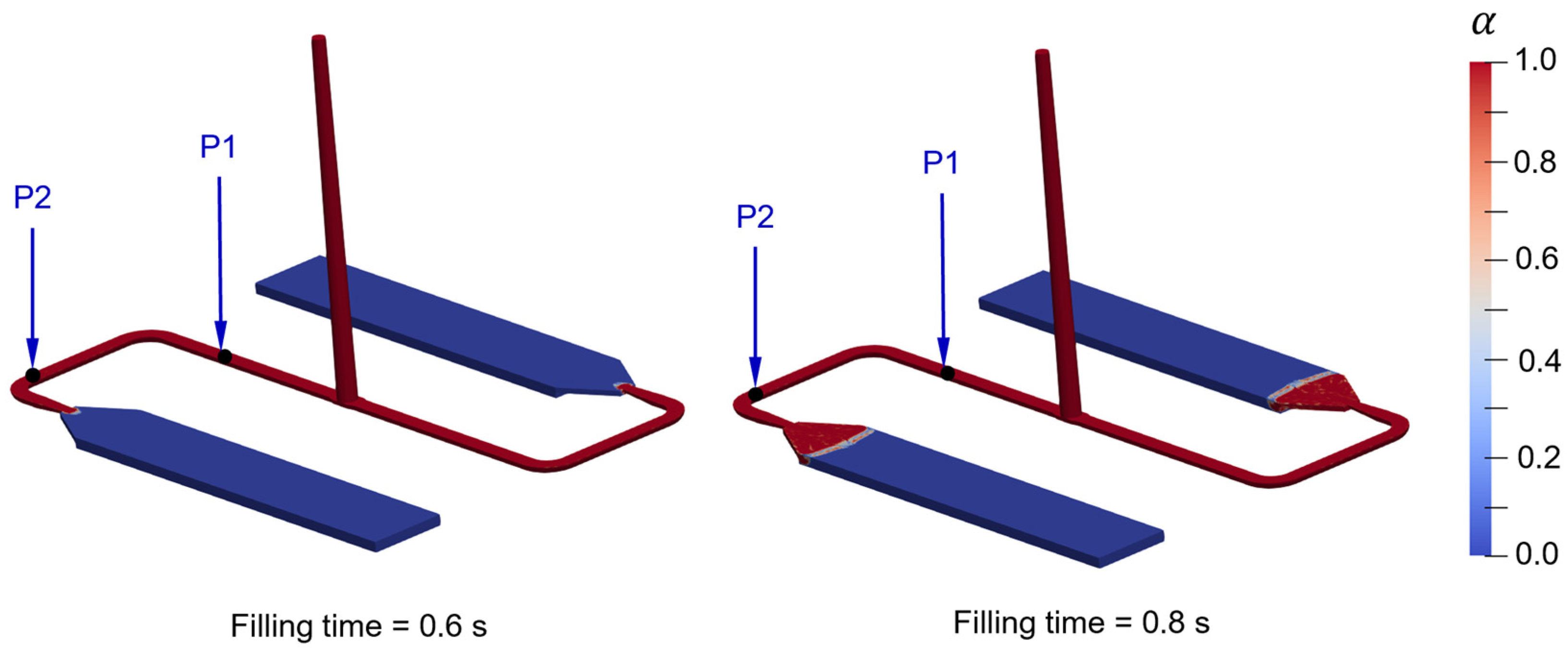
5.2. Validation of the Mold-Filling Simulations
6. Conclusions
Author Contributions
Funding
Data Availability Statement
Acknowledgments
Conflicts of Interest
References
- Gandhi, U.; Osswald, T.A.; Goris, S.; Song, Y.-Y.; Diaz Luque, J. Discontinuous Fiber-Reinforced Composites: Fundamentals and Applications, 1st ed.; Hanser Publications: Cincinnati, OH, USA, 2020; ISBN 978-1-56990-694-1. [Google Scholar]
- Shen, S.-F. Simulation of the Processing of Thermoset Polymers. Int. J. Numer. Methods Eng. 1990, 30, 1633–1647. [Google Scholar] [CrossRef]
- Osswald, T.A.; Turng, L.S.; Gramann, P.J. Injection Molding Handbook; Carl Hanser Publishers: Munich, Germany, 2008; ISBN 978-3-446-40781-7. [Google Scholar]
- Pickering, S.J. Recycling Thermoset Composite Materials. In Wiley Encyclopedia of Composites; John Wiley & Sons, Ltd.: Hoboken, NJ, USA, 2012; pp. 1–17. ISBN 978-1-118-09729-8. [Google Scholar]
- Olson, B.A.; De Keyser, H. Recycling Cured Phenolic Material. J. Thermoplast. Compos. Mater. 1994, 7, 30–41. [Google Scholar] [CrossRef]
- Torres, A.; de Marco, I.; Caballero, B.M.; Laresgoiti, M.F.; Legarreta, J.A.; Cabrero, M.A.; González, A.; Chomón, M.J.; Gondra, K. Recycling by Pyrolysis of Thermoset Composites: Characteristics of the Liquid and Gaseous Fuels Obtained. Fuel 2000, 79, 897–902. [Google Scholar] [CrossRef]
- Okajima, I.; Hiramatsu, M.; Shimamura, Y.; Awaya, T.; Sako, T. Chemical Recycling of Carbon Fiber Reinforced Plastic Using Supercritical Methanol. J. Supercrit. Fluids 2014, 91, 68–76. [Google Scholar] [CrossRef]
- Dorigato, A. Recycling of Thermosetting Composites for Wind Blade Application. Adv. Ind. Eng. Polym. Res. 2021, 4, 116–132. [Google Scholar] [CrossRef]
- Zhang, Y.; Pontikes, Y.; Lessard, L.; van Vuure, A.W. Recycling and Valorization of Glass Fibre Thermoset Composite Waste by Cold Incorporation into a Sustainable Inorganic Polymer Matrix. Compos. Part B Eng. 2021, 223, 109120. [Google Scholar] [CrossRef]
- Morici, E.; Dintcheva, N.T. Recycling of Thermoset Materials and Thermoset-Based Composites: Challenge and Opportunity. Polymers 2022, 14, 4153. [Google Scholar] [CrossRef] [PubMed]
- Domurath, J.; Saphiannikova, M.; Ausias, G.; Heinrich, G. Modelling of Stress and Strain Amplification Effects in Filled Polymer Melts. J. Non-Newton. Fluid Mech. 2012, 171–172, 8–16. [Google Scholar] [CrossRef]
- Wittemann, F.; Maertens, R.; Bernath, A.; Hohberg, M.; Kärger, L.; Henning, F. Simulation of Reinforced Reactive Injection Molding with the Finite Volume Method. J. Compos. Sci. 2018, 2, 5. [Google Scholar] [CrossRef]
- Tran, N.T.; Gehde, M. Creating Material Data for Thermoset Injection Molding Simulation Process. Polym. Test. 2019, 73, 284–292. [Google Scholar] [CrossRef]
- Wittemann, F.; Maertens, R.; Kärger, L.; Henning, F. Injection Molding Simulation of Short Fiber Reinforced Thermosets with Anisotropic and Non-Newtonian Flow Behavior. Compos. Part Appl. Sci. Manuf. 2019, 124, 105476. [Google Scholar] [CrossRef]
- Tran, N.T. Creating Material Properties for Thermoset Injection Molding Simulation Process. Ph.D. Thesis, Technische Universität Chemnitz, Chemnitz, Germany, 2020. [Google Scholar]
- Wittemann, F. Fiber-Dependent Injection Molding Simulation of Discontinuous Reinforced Polymers. Ph.D. Thesis, Karlsruher Institut für Technologie (KIT), Karlsruhe, Germany, 2022. [Google Scholar]
- Tran, N.T.; Gehde, M. Modelling of Rheological and Thermal Properties for Thermoset Injection Molding Simulation Process. In Proceedings of the 37th International Conference of The Polymer Processing Society (PPS-37), Fukuoka City, Japan, 11–15 April 2022; p. 110001. [Google Scholar]
- Tran, N.T.; Seefried, A.; Gehde, M. Investigation of the Influence of Fiber Content, Processing Conditions and Surface Roughness on the Polymer Filling Behavior in Thermoset Injection Molding. Polymers 2023, 15, 1244. [Google Scholar] [CrossRef]
- Domurath, J. Stress and Strain Amplification in Non-Newtonian Fluids Filled with Spherical and Anisometric Particles. Ph.D. Thesis, Technische Universität Dresden, Dresden, Germany, 2018. [Google Scholar]
- Favaloro, A.J.; Tseng, H.-C.; Pipes, R.B. A New Anisotropic Viscous Constitutive Model for Composites Molding Simulation. Compos. Part Appl. Sci. Manuf. 2018, 115, 112–122. [Google Scholar] [CrossRef]
- Karl, T.; Zartmann, J.; Dalpke, S.; Gatti, D.; Frohnapfel, B.; Böhlke, T. Influence of Flow–Fiber Coupling during Mold-Filling on the Stress Field in Short-Fiber Reinforced Composites. Comput. Mech. 2023, 71, 991–1013. [Google Scholar] [CrossRef]
- Farris, R.J. Prediction of the Viscosity of Multimodal Suspensions from Unimodal Viscosity Data. Trans. Soc. Rheol. 1968, 12, 281–301. [Google Scholar] [CrossRef]
- Sudduth, R.D. A Generalized Model to Predict the Viscosity of Solutions with Suspended Particles. I. J. Appl. Polym. Sci. 1993, 48, 25–36. [Google Scholar] [CrossRef]
- Wagner, N.J.; Woutersen, A.T.J.M. The Viscosity of Bimodal and Polydisperse Suspensions of Hard Spheres in the Dilute Limit. J. Fluid Mech. 1994, 278, 267–287. [Google Scholar] [CrossRef]
- Qi, F.; Tanner, R.I. Random Close Packing and Relative Viscosity of Multimodal Suspensions. Rheol. Acta 2012, 51, 289–302. [Google Scholar] [CrossRef]
- Dörr, A.; Sadiki, A.; Mehdizadeh, A. A Discrete Model for the Apparent Viscosity of Polydisperse Suspensions Including Maximum Packing Fraction. J. Rheol. 2013, 57, 743–765. [Google Scholar] [CrossRef]
- Farr, R.S. Simple Heuristic for the Viscosity of Polydisperse Hard Spheres. J. Chem. Phys. 2014, 141, 214503. [Google Scholar] [CrossRef]
- Mwasame, P.M.; Wagner, N.J.; Beris, A.N. Modeling the Effects of Polydispersity on the Viscosity of Noncolloidal Hard Sphere Suspensions. J. Rheol. 2016, 60, 225–240. [Google Scholar] [CrossRef]
- Roquier, G. Viscosity of Multimodal Concentrated Suspensions in a Newtonian Fluid. Acad. J. Civ. Eng. 2016, 34, 823–831. [Google Scholar]
- Mendoza, C.I. A Simple Semiempirical Model for the Effective Viscosity of Multicomponent Suspensions. Rheol. Acta 2017, 56, 487–499. [Google Scholar] [CrossRef]
- Mor Moshe Gottlieb, R.; Graham, A.; Mondy, L. Viscosity of Concentrated Suspensions of Sphere/Rod Mixtures. Chem. Eng. Commun. 1996, 148–150, 421–430. [Google Scholar] [CrossRef]
- Marti, I.; Höfler, O.; Fischer, P.; Windhab, E.J. Rheology of Concentrated Suspensions Containing Mixtures of Spheres and Fibres. Rheol. Acta 2005, 44, 502–512. [Google Scholar] [CrossRef]
- Domurath, J.; Saphiannikova, M.; Heinrich, G. Non-Linear Viscoelasticity of Filled Polymer Melts: Stress and Strain Amplification Approach. Macromol. Symp. 2014, 338, 54–61. [Google Scholar] [CrossRef]
- Domurath, J.; Saphiannikova, M.; Férec, J.; Ausias, G.; Heinrich, G. Stress and Strain Amplification in a Dilute Suspension of Spherical Particles Based on a Bird–Carreau Model. J. Non-Newton. Fluid Mech. 2015, 221, 95–102. [Google Scholar] [CrossRef]
- Ivaneyko, D.; Domurath, J.; Heinrich, G.; Saphiannikova, M. Intrinsic Modulus and Strain Coefficients in Dilute Composites with a Neo-Hookean Elastic Matrix. Appl. Eng. Sci. 2022, 10, 100100. [Google Scholar] [CrossRef]
- Westermaier, S.; Kowalczyk, W. Implementation of Non-Newtonian Fluid Properties for Compressible Multiphase Flows in OpenFOAM. Open J. Fluid Dyn. 2020, 10, 135–150. [Google Scholar] [CrossRef]
- Wittemann, F.; Kärger, L.; Henning, F. Influence of Fiber Breakage on Flow Behavior in Fiber Length- and Orientation-Dependent Injection Molding Simulations. J. Non-Newton. Fluid Mech. 2022, 310, 104950. [Google Scholar] [CrossRef]
- Castro, J.M.; Macosko, C.W. Studies of Mold Filling and Curing in the Reaction Injection Molding Process. AIChE J. 1982, 28, 250–260. [Google Scholar] [CrossRef]
- Einstein, A. Eine Neue Bestimmung Der Moleküldimensionen. Ann. Phys. 1906, 324, 289–306. [Google Scholar] [CrossRef]
- Batchelor, G.K.; Green, J.T. The Determination of the Bulk Stress in a Suspension of Spherical Particles to Order c 2. J. Fluid Mech. 1972, 56, 401–427. [Google Scholar] [CrossRef]
- Chhabra, R.P. Rheology: From Simple Fluids to Complex Suspensions. In Lignocellulosic Fibers and Wood Handbook; John Wiley & Sons, Ltd.: Hoboken, NJ, USA, 2016; pp. 405–438. ISBN 978-1-118-77372-7. [Google Scholar]
- Peker, S.M.; Helvacı, Ş.Ş. Solid-Liquid Two Phase Flow, 1st ed.; Elsevier: Amsterdam, The Netherlands; Oxford, UK, 2008; ISBN 978-0-444-52237-5. [Google Scholar]
- Krieger, I.M.; Dougherty, T.J. A Mechanism for Non-Newtonian Flow in Suspensions of Rigid Spheres. Trans. Soc. Rheol. 1959, 3, 137–152. [Google Scholar] [CrossRef]
- Ismail, I.; Vandenberg, J.; Abdala, A.; Macosko, C. Modeling the Intrinsic Viscosity of Polydisperse Disks. J. Rheol. 2017, 61, 997–1006. [Google Scholar] [CrossRef]
- Sudduth, R.D. Influence of Nanoscale Fibres and Discs on Intrinsic Modulus and Packing Fraction of Polymeric Particulate Composites and Suspensions. Mater. Sci. Technol. 2003, 19, 1181–1190. [Google Scholar] [CrossRef]
- Sudduth, R.D. A New Method to Predict the Maximum Packing Fraction and the Viscosity of Solutions with a Size Distribution of Suspended Particles. II. J. Appl. Polym. Sci. 1993, 48, 37–55. [Google Scholar] [CrossRef]
- Furnas, C.C. Grading Aggregates—I.—Mathematical Relations for Beds of Broken Solids of Maximum Density. Ind. Eng. Chem. 1931, 23, 1052–1058. [Google Scholar] [CrossRef]
- Kamal, M.R.; Sourour, S. Kinetics and Thermal Characterization of Thermoset Cure. Polym. Eng. Sci. 1973, 13, 59–64. [Google Scholar] [CrossRef]
- Wilczyński, K. Rheology in Polymer Processing: Modeling and Simulation; Hanser Publishers: Munich, Germany, 2021; ISBN 978-1-56990-660-6. [Google Scholar]
- Ostwald, W. Ueber die Geschwindigkeitsfunktion der Viskosität disperser Systeme. IV. Kolloid-Z. 1925, 36, 248–250. [Google Scholar] [CrossRef]


| Filler | Mean Diameter in m | Fillers’ Volume Fractions | |||
|---|---|---|---|---|---|
| Composition 1 | Composition 2 | Composition 3 | |||
| Glass fibers | 15.38 | 13 | 0.140 | 0.134 | 0.128 |
| Wollastonite | 45 | 12.5 | 0.328 | 0.313 | 0.298 |
| Silicon dioxide | 1 | 40 | 0.225 | 0.214 | 0.204 |
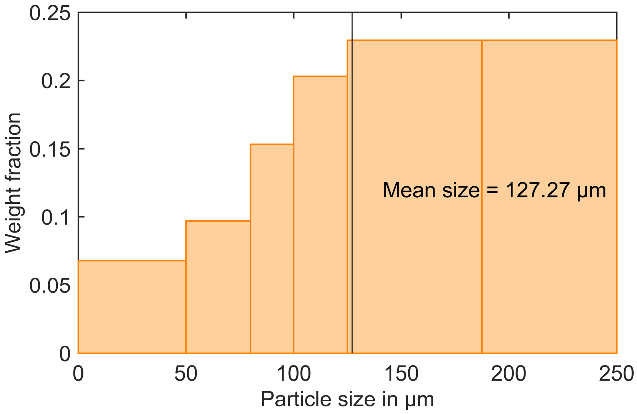
| RTC | 1 | 127.27 | 0 | 0.046 | 0.092 |
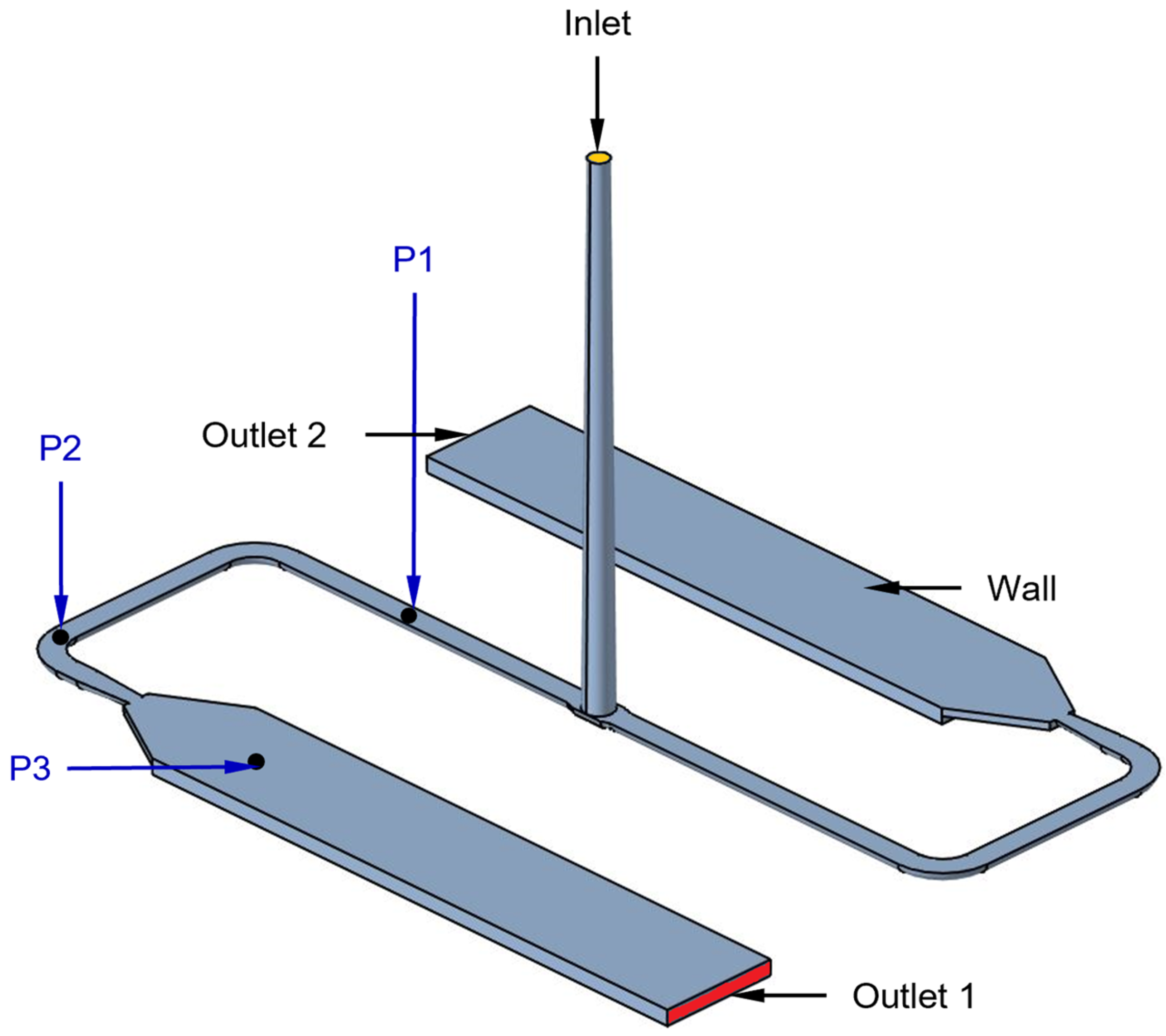
| Variable | Unit | Initial Internal Field | Inlet | Wall | Outlets 1 and 2 |
|---|---|---|---|---|---|
| - | 0 | fixedValue 1 | zeroGradient | zeroGradient | |
| 448.15 | fixedValue 378.15 | fixedValue 448.15 | zeroGradient | ||
| (0 0 0) | flowRateInletVelocity 10−5 or 1.5 × 10⁻⁵ | zeroGradient | zeroGradient | ||
| 105 | fixedfluxPressure 105 | fixedfluxPressure 105 | fixedfluxPressure 105 | ||
| 105 | fixedfluxPressure 105 | fixedfluxPressure 105 | fixedfluxPressure 105 | ||
| - | 0.001 | zeroGradient | zeroGradient | zeroGradient | |
| 0 | zeroGradient | zeroGradient | zeroGradient |
| Parameter | Value | Unit |
|---|---|---|
| 0.477 | ||
| 1.0595 | ||
| 1.5 × 10⁻⁸ | ||
| 15,500 | ||
| 4 | ||
| 44 | ||
| 0.4 |
| Parameter | Value | Unit |
|---|---|---|
| 8.314 | ||
| 9.55 × 10¹² | ||
| 0.0063 | ||
| 122,000 | ||
| 18,872.9 | ||
| 0.001 | ||
| 2.2 |
Disclaimer/Publisher’s Note: The statements, opinions and data contained in all publications are solely those of the individual author(s) and contributor(s) and not of MDPI and/or the editor(s). MDPI and/or the editor(s) disclaim responsibility for any injury to people or property resulting from any ideas, methods, instructions or products referred to in the content. |
© 2024 by the authors. Licensee MDPI, Basel, Switzerland. This article is an open access article distributed under the terms and conditions of the Creative Commons Attribution (CC BY) license (https://creativecommons.org/licenses/by/4.0/).
Share and Cite
Jetty, B.; Wittemann, F.; Kärger, L. Modeling Approach for Reactive Injection Molding of Polydisperse Suspensions with Recycled Thermoset Composites. Polymers 2024, 16, 2245. https://doi.org/10.3390/polym16162245
Jetty B, Wittemann F, Kärger L. Modeling Approach for Reactive Injection Molding of Polydisperse Suspensions with Recycled Thermoset Composites. Polymers. 2024; 16(16):2245. https://doi.org/10.3390/polym16162245
Chicago/Turabian StyleJetty, Bhimesh, Florian Wittemann, and Luise Kärger. 2024. "Modeling Approach for Reactive Injection Molding of Polydisperse Suspensions with Recycled Thermoset Composites" Polymers 16, no. 16: 2245. https://doi.org/10.3390/polym16162245
APA StyleJetty, B., Wittemann, F., & Kärger, L. (2024). Modeling Approach for Reactive Injection Molding of Polydisperse Suspensions with Recycled Thermoset Composites. Polymers, 16(16), 2245. https://doi.org/10.3390/polym16162245