Raising Two More Fundamental Questions Regarding the Classical Views on the Rheology of Polymer Melts

Abstract

The current paradigm of polymer flow assumes that (i) the effect of the molecular weight of the macromolecules, M, and of the temperature, T, on the expression of the viscosity of polymer melts separate; (ii) the molecular weight for entanglement, M_c, is independent of T; and (iii) the determination of M_c by the break in the log viscosity curve against log M unequivocally differentiates un-entangled melts from entangled melts. We use reliable rheological data on monodispersed polystyrene samples from very low molecular weight (M/M_c = 0.015) to relatively high molecular weight (M/M_c = 34) to test the separation of M and T in the expression of the viscosity; we reveal that an overall illusion of the validity of the separation of T and M is mathematically comprehensible, especially at high temperature and for M > 2M_c, but that, strictly speaking, the separation of M and T is not valid, except for certain periodic values of M equal to M_c, 2M_c, 4M_c, 8M_c, 16M_c, etc. (period doubling) organized around a “pole reference” value M_R = 4M_c. We also reveal, for M < M_c, the existence of a lower molecular weight limit, M’_c = M_c/8 for the onset of the macromolecular behavior (macro-coil). The discrete and periodic values of M that validate the separation of the effect of M and T on the viscosity generate the fragmentation of the molecular range into three rheological ranges. Likewise, we show that the effect of temperature is also fragmented into three rheological ranges for T > T_g: T_g < T< (T_g + 23°), (T_g + 23°) < T < T_LL and T > T_LL’ where T_LL is the liquid-liquid temperature. Our conclusion is that the classical formulation of the viscosity of polymer melts is so overly simplified that it is missing important experimental facts, such as period doubling for the separation of T and M, T_LL, M’_c, and M_c, resulting in its inability to understand the true nature of entanglements. We present in the discussion of the paper the alternative approach to the viscoelastic behavior, “the duality and cross-duality” of the Dual-conformers, showing how this model formalism was used to test mathematically and invalidate the separation of T and M in the classical formulation of viscosity.

1. Introduction

Polymers are made up of long-chain molecules, which have been studied for more than 70 years, leading to our current understanding of how they flow under stress at high molding temperatures [1]. Viscosity, the stress divided by the strain rate, is the physical variable to follow to describe the effect of the molecular weight of the macromolecules, M, and of the temperature, T, on the ability of the polymer melts to flow in molds, extruders and injection molding machines. Fundamentally, the current paradigm of polymer flow [1] relies on assumptions made at the beginning of the investigations in polymer science that have rarely been questioned, if they ever were:

• Is the separation of the M and T variables in the expression of the viscosity truly validated?
• Is the molecular weight for entanglement, M_c, truly independent of T, and is the determination of M_c by the break in the log viscosity curve against log M, unequivocally assigned to characterize “entanglements”?

The objective of this communication is to provide qualified experimental and mathematical evidence to be able to answer both questions. We analyze reliable rheological data [2,3] on a series of monodispersed polystyrene samples from very low molecular weight (M/M_c = 0.015) to relatively high molecular weight (M/M_c = 34). The qualification of these data is critically examined. Our tentative conclusions lead to answer no to both questions, yet their generalization will require that the experiments be repeated and extended to include more molecular weight samples. This new tentative invalidation of the currently accepted views in the rheology of polymer melts comes after the publication [4] of inconsistencies found in the two most popular dynamic models of the rheology of melts, the Rouse model [5] and the reptation model [6].

In the Development section, we show that our viscosity equation explains the appearance of validity of the separation of T and M, especially at high temperature and for M > 2M_c, but invalidates, strictly speaking, the separation of M and T except for certain periodic values of M equal to M_c, 2M_c, 4M_c, 8M_c, etc. (period doubling) organized around a “pole reference” value M_R = 4M_c. This paper also suggests, for M < M_c, the existence of a lower molecular weight limit, M’_c = M_c/8 that we assign to the onset of the macromolecular behavior (the formation of stable macro-coils). The discrete and periodic values of M that validate the separation of the effect of M and T on the viscosity generate the fragmentation of the molecular range into three rheological ranges for M > M’_c and/or M > M_c as well as the fragmentation of the temperature range above T_g into three rheological ranges: T_g < T < (T_g + 23°), (T_g + 23°) < T < T_LL, and T > T_LL, where T_LL is the liquid-liquid temperature [4,7,8,9,10,11,12]. This fragmentation of the rheological data range challenges the classical claims that molecular motions involving the macromolecules occur identically over the full temperature and that the molecular range is only fragmented into two ranges by M_c. We introduce in the Discussion section the reasons that led to the formulation of the empirical viscosity equation used to test the separation of M and T and explain how their conception was inspired by the dual-split general concepts and the simulation work specifically done to simulate viscosity [7,8,9].

Figure 1 schematically summarizes the classical description of the rheology of polymer melts. Our disruptive new perspective of the effect of M and T to characterize the changes of viscosity presented in this paper reinforces what we already suggested somewhere else [4,10] that the current rheology paradigm has overly simplified the presentation of the experimental facts, perhaps to be able to understand them within the current paradigm framework, and has defensively declared artifacts any experimental deviation from their expectations when there was no possible explanation for those facts by the current paradigm. In our discussion, we briefly present “the duality and cross-duality” of the Dual-conformers, an alternative approach to the viscoelastic behavior of polymer macromolecules. In this new physics of polymer interactions, the Dual-conformers belong to the same macromolecule or different ones and assemble as dissipative open statistical systems of interactions [4,7,8,9]; we conclude that this model explains, at least qualitatively, all the new and provocative results regarding the effect of M and T on the viscosity introduced and analyzed in this paper.

2. Development

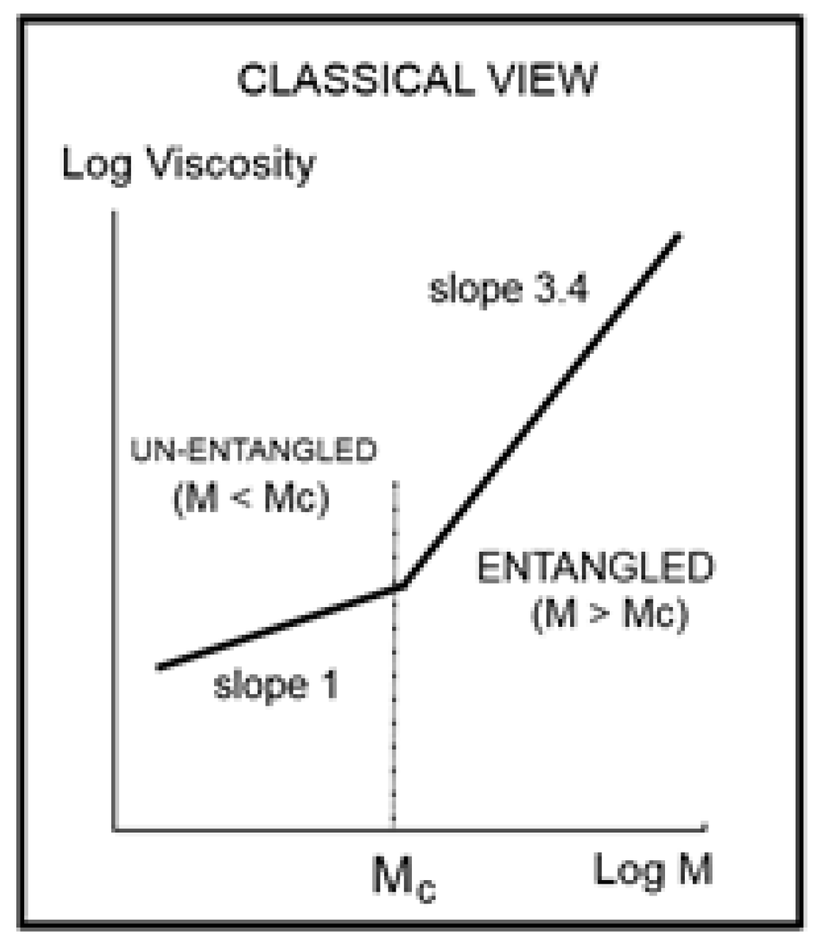
The fundamental classical understanding of polymers’ rheology can be summarized in one graph, shown in Figure 1. This plot of the log of the “Newtonian” viscosity (viscosity extrapolated at an infinitely small shear rate) against the log of the molecular weight of the macromolecule, log M, is done at constant temperature or at constant free volume, proportional to T − T_g, to account for the molecular weight dependence of T_g (only affecting the M < M_c data since T_g is quasi-constant above M_c). Such a plot is shown, for instance, on p. 50 (Figure 5.4) of Graessley [1]. Figure 1 separates two distinct regions, an “ENTANGLED” region, with a slope of 3.4 for the log μ_o vs. log M and an “UN-ENTANGLED” region with a slope of 1. The two regions are separated by M_c, the molecular weight for entanglements. The large increase in the effect of the molecular weight on the viscosity is remarkably stated by the increase of the slope from 1 to 3.4, which occurs for M > M_c. The concept of “entanglement” in polymers was derived from figuring out why a sharp break in the viscosity occurred at M_c in Figure 1, separating the shorter molecular weights from the longer molecular weights. When the temperature is changed to a different value, Figure 1 remains basically unchanged, except for a vertical shift of the lines, their slopes remaining constant to their respective values across M_c, and their intersection’s x-coordinate also remaining constant at M_c’. As a consequence, the Newtonian viscosity μ_o is the product of two independent terms, one varying with temperature only, T, and the other one with molecular weight only, M. This is what is designated by “the separation of M and T in the expression of viscosity”. Generally speaking, the experimental evidence backing up the veracity of the features in Figure 1 is overwhelming and has been verified and agreed to by a multitude of qualified peers throughout the literature [1]. The authors of the data that we re-analyze in this paper, Dr. Pierson and Dr. Susuki [2,3] verified and explicitly claimed that their data validated the classical formula, thus the separation of M and T; they compared their data to other researchers’ data, again claiming a complete compatibility. Using a different perspective than classical, this author also examined closely the experimental results in [2,3] and reported in [10] and Chapter 3 of [7], the impact of the measurement uncertainties on the slopes, intercepts, and the determination of M_c at their intersection in Figure 1 for the data of Pierson and Susuki. It was reported in [7,10] that what is shown here as Figure 1 was, indeed, “visually observed”, providing the apparent validation of the classical approach. Furthermore, several researchers of the University of Pau and Pays de l’Adour (UPPA) [13,14,15,16] worked on the rheology of monodispersed Polystyrene polymers to study their blends [13,15,16] or validate rheological models based on tube dynamics [15], and compared their results with those done previously by other scientists, explicitly validating their results with those of Pierson and Susuki. In summary, the data of Susuki and Pierson, reanalyzed in the present paper from another angle than the classical rheological approach, are reliable results: they have been verified by us and by several authors who have all claimed the validation of the classical view. The only difference between our own conclusion and these authors’ conclusions was the presence of the word “apparent” before validation in our conclusion.

This paper is divided into three sections: in the first section (A), illustrated by Figure 2, Figure 3, Figure 4, Figure 5, Figure 6, Figure 7 and Figure 8, we analyze Newtonian viscosity data plotted like in Figure 1 at various temperatures, showing that the classical picture of the effect of T and M on the viscosity and on the definition of M_c depicted by Figure 1 may be incomplete and too simplistic to be practically useful and leads to the wrong conclusions regarding the nature of entanglements. In the second section (B), illustrated in Figures 9–21, we introduce a new empirical formulation of the viscosity (inspired by the Cross-Duality concept) to address the testing of the separation of M and T. This mathematical formula quantitatively describes the viscosity data “perfectly” (r² = 1.0) when M and T vary and can be plotted like in Figure 1 to determine the slopes projected by the classical formulation of viscosity (Figure 1). This mathematical fitting exercise reveals the invalidation of the separation of M and T except at values of M corresponding to period doubling multiples of M_c. We also conclude in section (B) on the futility of finding a theoretical explanation for the value of the slopes, 1 and 3.4, respectively, for M < M_c and M > M_c in Figure 1. Finally, in the last section (Discussion), we point to the main differences between the admitted polymer dynamic models’ approach to mechanical flow and our disruptive model of polymer interactions that is manifested by a new interpretation of the viscoelastic effects and entanglements.

A.

The Effect of Molecular weight on the Newtonian Viscosity at various constant T.

Figure 2, Figure 3, Figure 4, Figure 5, Figure 6 and Figure 7 plot Log (μ_o) vs. Log (M/M_e) data obtained at various temperatures for a series of monodispersed Polystyrene (PS) samples. μ_o is the Newtonian viscosity (in Poises), and M_e is the molecular weight between entanglements, known to correspond to ~M_c/2 where M_c demarks the break between the un-entangled and entangled data in Figure 1. The data were first generated and analyzed by Pierson in his PhD thesis at the University of Strasbourg [2]. The same monodispersed PS samples were part of an extended study and retested by Susuki [3], also at the University of Strasbourg, revealing an excellent repeatability of the results of Pierson and a concurring analysis using the classical formula of rheology. As already mentioned, Pierson and Susuki’s viscosity results on monodispersed PS were tested and validated over the years by several scientists at the university of Pau and Pays de l’Adour (UPPA), for instance, by Majeste [16], Montfort [13], Marin [14], and Cassagnau [15]. The Susuki’s data will be used in section B of the paper because it involves more samples with M > M_c. Theses authors adhered to the established practice of the separation of the effect of T and M during their analysis. This provides an excellent example of rheological data that can be analyzed with an “apparent great satisfaction” according to the classical views, yet with great concerns when our approach analyzes the same data from a different angle. For instance, Pierson and Susuki use the Vogel-Fulcher equation and the WLF equations (Equations (1) and (2)) to express the temperature dependence of the friction factor of the Newtonian viscosity at constant M.

Logμ_o = A + B/(T − T2)

(1)

where A, B, and T₂ are fitting parameters that vary with M [1,17]. This equation can be rewritten with respect to a temperature reference, for instance, T_g at which the viscosity is μ_og:

log (μ_o/(μ_og) = −C_1g(T − T_g)/(C_2g + (T − T_g)

(2)

with

C_1g = B/(T_g– T₂) and C_2g = (T_g − T₂)

(3)

where the fitting constants, C_1g and C_2g are often called the WLF constants [1,17]. The viscosity is now expressed as a function of the free volume, proportional to (T − T_g). The validity of the Vogel-Fulcher and the WLF equations over the temperature range is restricted by the classical models to hold between T_g to (T_g + 100°); beyond that, Equation (1) is often replaced by a thermally activated expression providing an Arrhenius description of the temperature dependence of the Newtonian viscosity Chapter 11 of [17]. The fragmentation of the rheological data into two ranges has been critically reviewed by this author in several publications [10,11,12], Chapter 3 of [6]; it is also an important issue raised in the present communication.

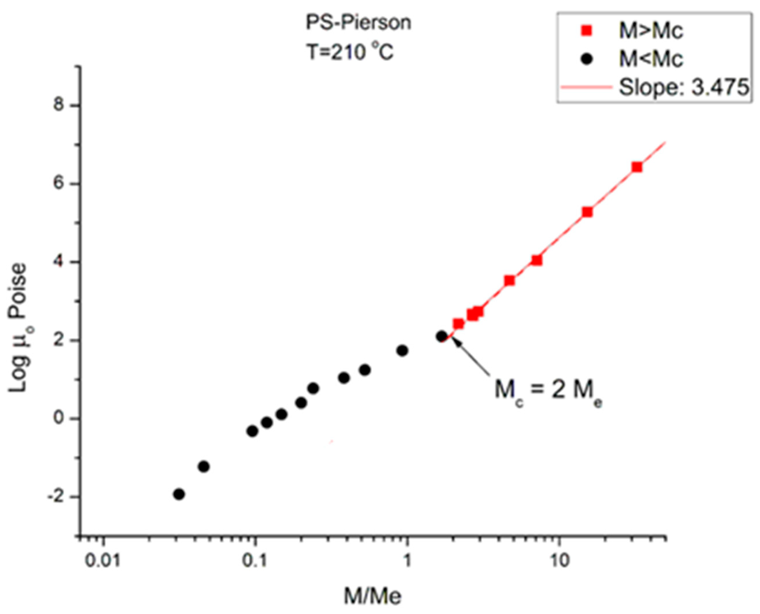
Figure 2 corresponds to the data of Pierson [2] at T = 210 °C plotted pursuant to Figure 1. The unit for viscosity is Poise (i.e., 0.1 Pa-s). The x axis is log (M/M_e) where M_e ~ M_c/2. The value of M_e is equal to ρRT/G_N pursuant to the theory of rubber elasticity where ρ is the melt density; R is the gas constant; T is the absolute temperature; and G_N is the plateau elastic modulus of an entangled melt [1,4]. We use red square symbols for M > M_c and dark dots for M < M_c. Above M_c, the data conform with what is classically expected: the log-log plot is a straight line with slope = 3.475 and intercept 1.164.

Figure 2. logμ_o(M) versus M/Meplotted pursuant to Figure 1. Data of Pierson [2] at T = 210 °C.

Figure 2. logμ_o(M) versus M/Meplotted pursuant to Figure 1. Data of Pierson [2] at T = 210 °C.

Below M_c, the log-log plot of the data should be a straight line with slope 1 according to classical predictions; instead, the dark dots align according to a curve more or less smoothly. This curvature, apparently contradicting the prediction of the Rouse model of the Newtonian viscosity proportionality to M for un-entangled polymers (M < M_c), has been reported and explained by several authors [1,10,16,17], chapter 3 of [6]. In particular, it was pointed out, as an explanation, that working at constant free volume instead of constant temperature would re-establish the proportionality between μ_o and M [1,10,17]. It is clear in Figure 2 that the general understanding of the effect of increasing the molecular weight conforms to what is predicted by the molecular dynamic models: 1. the longer the chains, the more difficult it is to shear them; 2. “entanglement” results in a significant increase in the difficulty to process polymer melts because of the increase of the viscosity by a ratio at least equal to M^2.4 (i.e., M^3.4/M), which is the ratio of the viscosity of an entangled melt to the viscosity of the same melt without entanglements present (a so-called disentangled melt) at the same temperature and for the same molecular weight M.

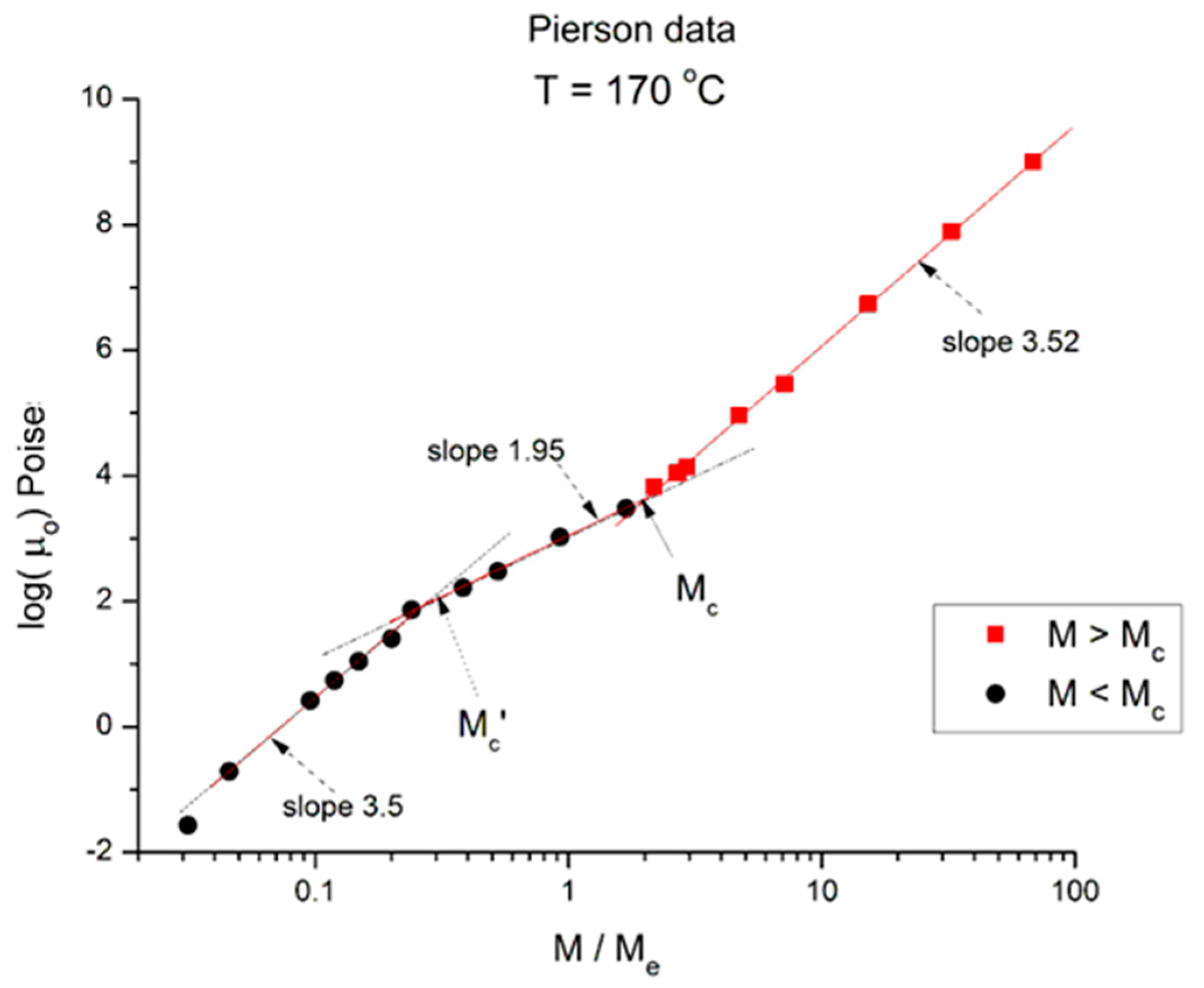
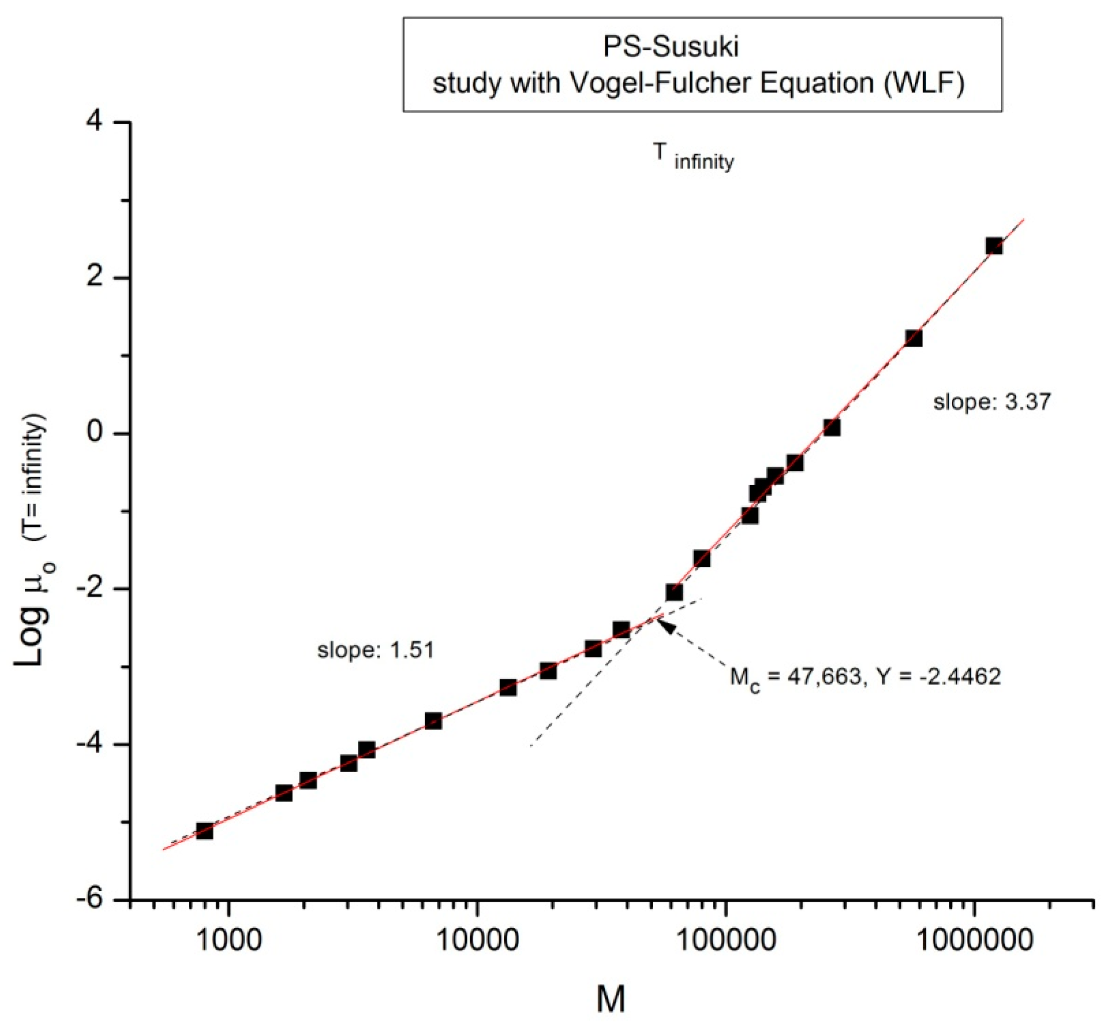
We now examine the same data but plotted at other temperatures T = 170 °C in Figure 3, T = 145 °C, 125 °C, 115 °C in Figure 4, Figure 5 and Figure 6, respectively. Finally, Figure 7 provides the value of the Newtonian viscosity versus M when T becomes infinity in the Vogel-Fulcher equation: T = ∞ → Logμ_o = A.

Figure 3. Logμ_o (M) at T = 170 °C plotted pursuant to Figure 1. Data of Pierson [2].

Figure 3. Logμ_o (M) at T = 170 °C plotted pursuant to Figure 1. Data of Pierson [2].

Essentially, Figure 3 can be compared to Figure 2 by saying that it is the same figure with a new look at considering the M < M_c data, in particular in the way the un-entangled range is broken down into two log-log lines instead of assuming it was a smooth curve in Figure 2. In fact, in the other Figure 4, Figure 5 and Figure 6, we follow this attempt to break down the low molecular weight region and compare the changes occurring to the slopes of the log-log straight lines thus defined.

In Figure 3 we have three straight line “sections” with slope, from left to right: 3.5, 1.95, and 3.52. The molecular weight delimitating the sections are M’_c, between range 1 and 2, and M_c between range 2 and 3, respectively. We see that (M’_c/M_e) ~ 0.25 and (M_c/M_e) ~ 2. The slope for the entangled data (the red squares) is not very different at T = 170 °C and at T = 210 °C, and the difference may look insignificant, proving that the separation of the effect of M and T would hold in this region. However, a fine study of this effect shows that the slope not only does not remain constant but systematically varies with T in a small yet continuous way (see Figure 8). The slope of 3.5 found for the first seven lower molecular weights is as big as that found in the entangled region. Why would the viscosity of low molecular weight “un-entangled” PS samples increase with M like M^3.5, an exponent thought to be characteristic, precisely, to the presence of entanglements?

Figure 4. Logμ_o (M) data of Pierson [2] at T = 145 °C plotted pursuant to Figure 1.

Figure 4. Logμ_o (M) data of Pierson [2] at T = 145 °C plotted pursuant to Figure 1.

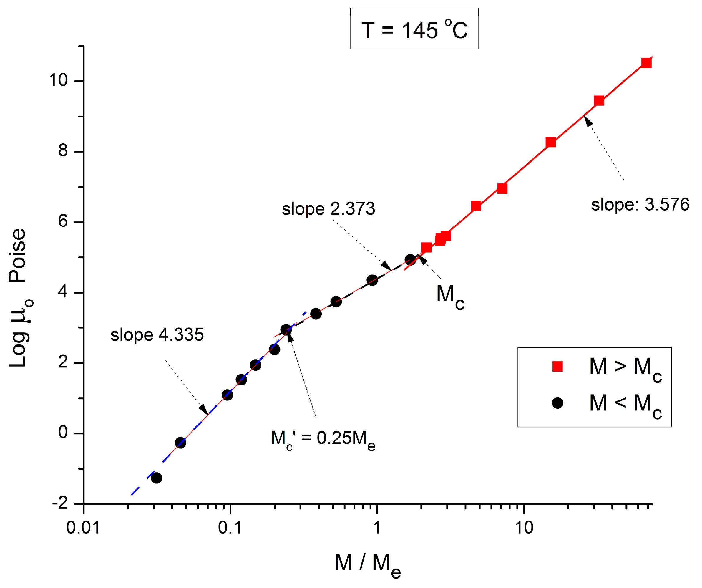
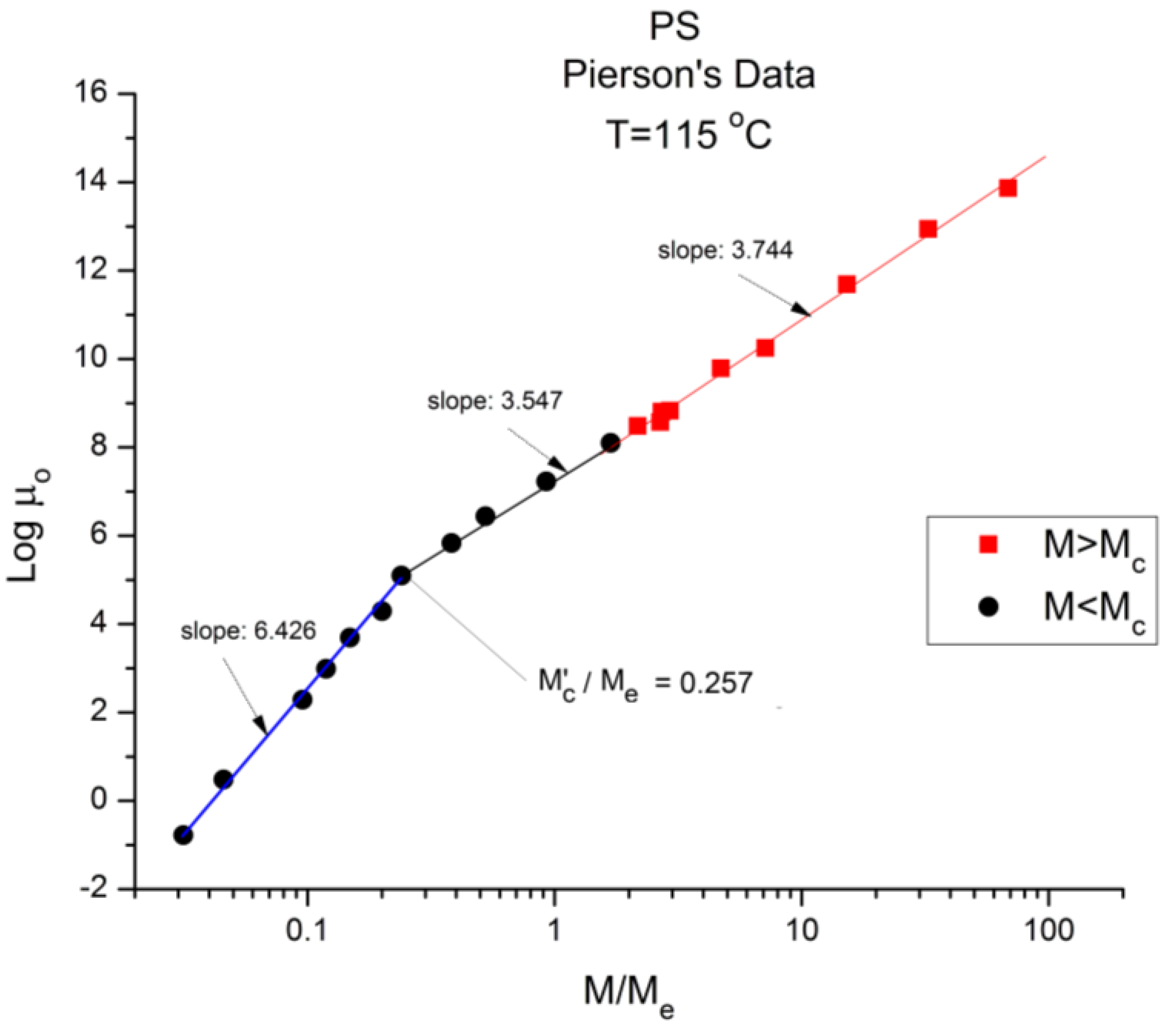
Figure 4 applies to T = 145 °C, showing the three regions and their respective slopes, from left to right: 4.335, 2.373, and 3.576, respectively. The breaks occur at M’_c = 0.25 M_e and M_c = 2 M_e. Figure 5 and Figure 6, for T = 125 °C and 115 °C, respectively, are different because they only reveal two log-log straight lines, not 3. The originality is the absence of the break at M = M_c! The slope in region 1, for M < 0.25 M_e, continues to sharply increase as T decreases, 6.0 for 125 °C, 6.38 for 115 °C. The slope in region 3, for M > M_c, continues to increase slightly as T decreases: 3.61 for T = 125 °C, and 3.63 for T = 115 °C. As already mentioned, this slope is not independent of T, as it should be to validate the separation of M and T in the formulation of the Newtonian viscosity. It is remarkable that Figure 5 and Figure 6 show no entanglement break from M = 0.25 M_e to 100 M_e, raising legitimate concerns regarding the concept of entanglement and its origin.

Additionally, the meaning of the slopes of Logμ_o vs. Log M themselves raise questions, including in the entanglement section of M. The traditional approach considers the change of the value of the exponent, typically from 1 to 3.4, to be important, even essential, to characterize the molecular weight dependence of viscosity. What about if this exponent turns out to be the wrong variable to tell what happens to the statistical properties of a set of macromolecules when their molecular weight increases?

Figure 5. Logμ_o (M) data of Pierson [2] at T = 125 °C plotted pursuant to Figure 1.

Figure 5. Logμ_o (M) data of Pierson [2] at T = 125 °C plotted pursuant to Figure 1.

Figure 6. Logμ_o (M) data of Pierson [2] at T = 115 °C plotted pursuant to Figure 1. The regressions consider the 2 ranges across M_c separate. If we fit one single range starting from M’_c the slope is 3.604 (r² = 0.998).

Figure 6. Logμ_o (M) data of Pierson [2] at T = 115 °C plotted pursuant to Figure 1. The regressions consider the 2 ranges across M_c separate. If we fit one single range starting from M’_c the slope is 3.604 (r² = 0.998).

Figure 7. Log μ_o (M) data of Pierson [2] at T extrapolated to ∞ and plotted pursuant to Figure 1.

Figure 7. Log μ_o (M) data of Pierson [2] at T extrapolated to ∞ and plotted pursuant to Figure 1.

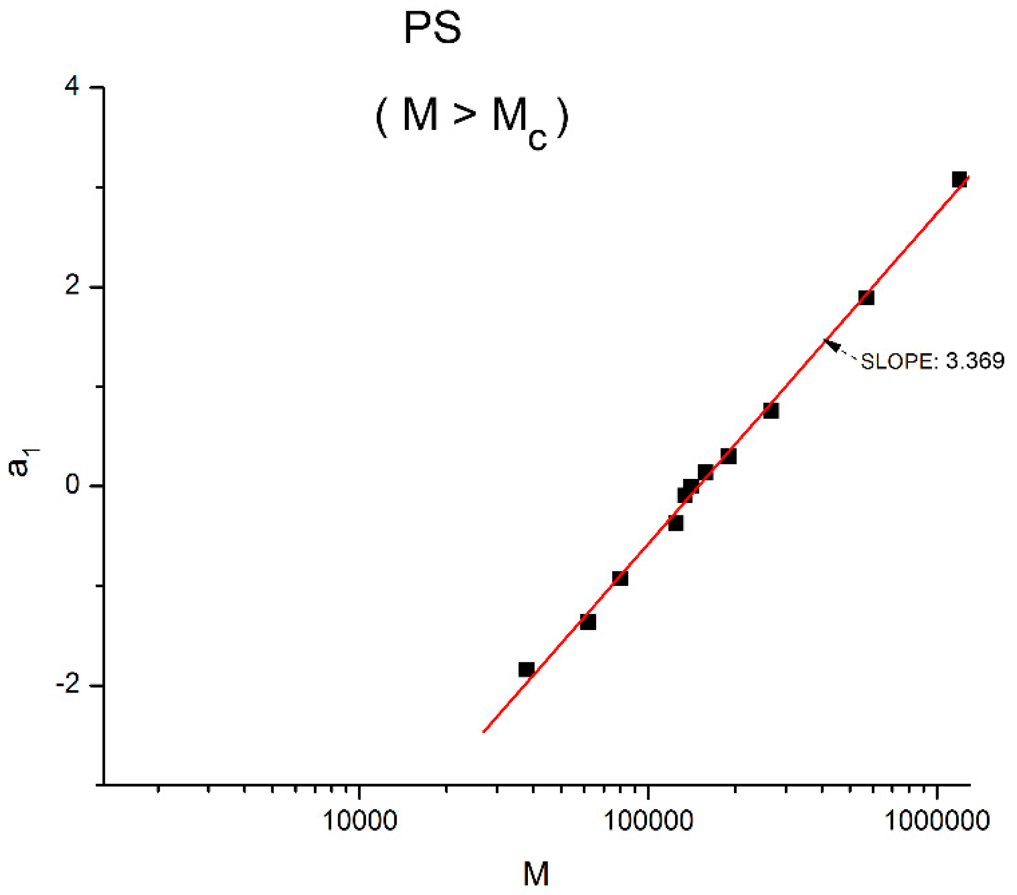
Take Figure 7 for instance: it is a plot of Log μ_o vs. Log M for T = ∞ in the Vogel-Fulcher equation. This figure could be used as a perfect illustration of the teaching of the classical views regarding entanglements: two regions of M are visible, well separated, and well described by the classical tools, with a slope of 3.37, almost perfectly 3.4, above M_c, and a slope of 1.5 below M_c. Although the slope below M_c is not 1, with possible reasons given before, the break between the high and low molecular weights is sharp and well defined. The problem, though, is that the M_c value at this sharp break, M_c = 47,663, is significantly greater (+36%) than the M_c~ 35,000 classically assigned to the molecular weight for entanglements for PS, p.55 [1]. Figure 2 correctly shows M_c at 35,000 for the same data. Would this be a sign to indicate that M_c varies with T, which it should not do according to the classical paradigm? Figure 5 and Figure 6 show the break in the viscosity curve occurring at 0.25 M_e, not 2M_e as projected by the classical explanation of entanglements. One sees that using the break in the viscosity curve to define M_c, like it is illustrated in Figure 1, is not coherent with the claim that M_c does not vary with temperature: Figure 5, Figure 6, and Figure 7 provide clear evidence that the value of M_c varies with T when it is defined by the break of the log viscosity-logM curve (Figure 1). An alternative explanation is based on the instability of the entanglement state [18], resulting in the possibility of manipulating the value of M_c, refer to the chapter 8 of [7].

Finally, there is the question of the meaning of M’_c~0.25 M_e = M_c/8 = 4375 g/mole. This molecular weight stands out in all the figures, separating the very low M and the region below M_c. Both Pierson [2] and Susuki [3] admit the existence of a deviation from the standard analysis in this region without raising the possibility of a molecular transition. To the best of our knowledge, the recognition of such a deviation as a true “molecular transition” below M_c has never been reported in the literature, except recently while analyzing T_LL (M) in Ref. [12]. The molecular weight of a monomeric repeat unit for PS is 104.15 g/mole, and M’_c corresponds to 42 such units. As T decreases from Figure 2, Figure 3, Figure 4, Figure 5, Figure 6 and Figure 7 from T infinity to T = 115 °C, respectively, the slope of log μ_o vs. M in the region M < M’_c monotonically increases from 1.5 to 6, a four-fold increase of the exponent of the effect of M on viscosity. It is clear that the admitted validation of the separation of the effect of M and T on viscosity badly fails in this region.

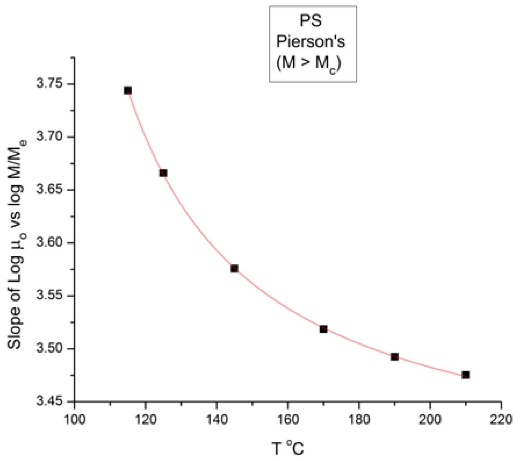
Figure 8 is a plot of the slope of log μ_o vs. M in the entanglement region (i.e., for M > M_c) in Figure 1. The classical value of the slope is 3.4, as said earlier, yet Figure 8 shows that, although the value of the slope is not far from 3.4, it is not constant when T increases and, even more problematically, it decreases monotonously, not randomly, from 3.635 at T = 115 °C to 3.475 at 210 °C, a clear indication that the exponent does not strictly remain constant when T varies. As we reported earlier, such a small change in the slope is not easily visually perceptible, giving the illusion of a constant slope for M > M_c when T varies. A regression analysis performed in the M > M_c range at various T unequivocally produces a small but systematic non-randomness of the deviation from 3.4 (or from whatever average value is chosen). Figure 8, already presented in a previous paper [10], was our first exposure to the possible failure of the separation of T and M in the expression of the viscosity, an indication that motivated the research presented in this communication. The second section of this paper, section B, will quantitatively explain the conditions rendering the effect of M and T on the viscosity separable.

Figure 8. Slope of Log μ_o vs. M in the entanglement region (i.e., for M > M_c) in Figure 1.

Figure 8. Slope of Log μ_o vs. M in the entanglement region (i.e., for M > M_c) in Figure 1.

We conclude from Figure 2, Figure 3, Figure 4, Figure 5, Figure 6, Figure 7 and Figure 8 that the basic foundation of the classical understanding of the effect of molecular weight and temperature on the Newtonian viscosity of polymer melts (Figure 1) is possibly contradicted by the above observations. To pursue this idea that the classical views might have oversimplified the effect of M and T in the formulation of the melt viscosity of polymers, we present in section B a mathematical demonstration that allows us to determine whether the effect of M and T on the viscosity do separate or not.

B

TESTING MATHEMATICALLY THE SEPARATION OF M AND T IN THE EXPRESSION OF VISCOSITY.

B1

Summary of the classical approach.

For polymers of low molecular weight (M < M_c) in Figure 1, the Newtonian viscosity takes the form:

μ_o(M,T) = K(T) M   (M < M_c)

(4)

where M is the molecular weight of the chains, μ_o is the Newtonian viscosity at temperature T, and K is a constant that varies with (T − T_g) to make the free volume constant in Equation (3). Note that the slope of 1 in Figure 1 for M < M_c requires in Equation (4) that K(T) be actually K(T − T_g) to work at free volume constant, where T_g is a function of M below M_c (i.e., T_g(M)). This means that the classical viscosity equation below M_c admits that M and T do not separate. This should be pointed out.

For longer chains (M > M_c), the classical and quasi-universal value of 3.4 reflects the power law dependence of the entanglements on the viscosity:

μ_o (M,T) = K’(T) M^3.4    (M > M_c)

(5)

The critical molecular weight, M_c’ is obtained from intersecting the straight lines Log μ_o vs. Log M drawn in the two regions M < M_c and M > M_c.

Formula (5) simply states that molecular weight and temperature effects separate in the expression of the viscosity of polymer melts. Since T_g is constant for M > M_c, K’(T − T_g) does not make this term function of M, unlike for M < M_c. The temperature dependence of K(T) or K’(T) in Equations (4) and (5) is often written, as we already said, with the WLF expression in Equation (3). The WLF equation explains the curvature observed in Arrhenius plots of log(μ_o) vs. 1/T and is claimed to work well between T_g and T_g + 100, with the reservations made previously regarding the veracity of that statement. The constants C_1g and C_2g in Equation (3) are often admitted to have the universal value of 17.44 and 51.6, respectively, a statement discussed and refuted in a previous communication [10]; in fact, it was shown that C_1g and C_2g are not constant when M is varied and that their molecular dependence revealed the fragmentation of the rheological range, an observation that will also be forthcoming from the Dual-Phase approach presented next.

B2

The Dual-Phase Inspired Approach.

Let us consider Equations (6) and (7), inspired by the classical formulation of rheology, yet modified pursuant to the two-phase nature of the Dual-conformers. This formulation of the effect of M and T on the Newtonian viscosity is empirical, as much as Formulas (4) and (5) are also empirical. The main difference between the classical empirical formula, (4) and (5) and the Dual-Phase inspired empirical formula, (6) and (7), is in the interpretation of the physical parameters entering the equations. This will be explained in the Discussion. In the following, we refer to “phase 1” and “phase 2” or their respective Newtonian viscosity, μ_o1 and μ_o2 pursuant to our assumption of a possible “split” of Logμ_o into a structure: Logμ_o1 and Logμ_o2, corresponding to (μ_o = μ_o1*μ_o2). The split is expressed in the first line of Equation (6):

$$\begin{array}{l}\mathrm{Log}{\mu }_{\mathrm{o}}(\mathrm{T},\mathrm{M})={\mathrm{a}}_1(\mathrm{M},\mathrm{T})+\mathrm{Log}{\mu }_{\mathrm{o}}\mathrm{R}\left(\mathrm{T}\right)=\mathrm{Log}{\mu }_{\mathrm{o}1}(\mathrm{T},\mathrm{M})+\mathrm{Log}{\mu }_{\mathrm{o}2}(\mathrm{T},\mathrm{M})\\ {\mathrm{a}}_1(\mathrm{M},\mathrm{T})={\mathrm{a}}_{11}(\mathrm{M},\mathrm{T})+{\mathrm{a}}_{12}(\mathrm{M},\mathrm{T})\\ \mathrm{Log}{\mu }_{\mathrm{o}1}(\mathrm{T},\mathrm{M})={\mathrm{a}}_{11}(\mathrm{M},\mathrm{T})+\mathrm{Log}{\mu }_{\mathrm{o}1}\mathrm{R}\left(\mathrm{T}\right)\\ \mathrm{Log}{\mu }_{\mathrm{o}2}(\mathrm{T},\mathrm{M})={\mathrm{a}}_{12}(\mathrm{M},\mathrm{T})+\mathrm{Log}{\mu }_{\mathrm{o}2}\mathrm{R}\left(\mathrm{T}\right)\\ \mathrm{Log}{\mu }_{\mathrm{o}}\mathrm{R}\left(\mathrm{T}\right)=\mathrm{Log}{\mu }_{\mathrm{o}}(\mathrm{T},\mathrm{M}={\mathrm{M}}_{\mathrm{R}})\end{array}$$

(6)

where the sub-index “11” refers to phase 1 and “12” to phase 2. When a₁(M,T) = a₁(M), Log μ_o(T,M) expresses the separation of M and T:

$$\begin{array}{l}{\mathrm{a}}_{12}={\mathrm{b}}_1+{\mathrm{b}}_2\exp (\Delta {\mathrm{H}}_{2\mathrm{R}}/\mathrm{T})+{\mathrm{b}}_4\exp (\Delta {\mathrm{H}}_2/\mathrm{T})\\ {\mathrm{a}}_{11}={\mathrm{b}’}_1+{\mathrm{b}’}_2\exp (\Delta {\mathrm{H}}_{1\mathrm{R}}/\mathrm{T})+{\mathrm{b}’}_4\exp (\Delta {\mathrm{H}}_1/\mathrm{T})\end{array}$$

(7)

where ΔH_2R and ΔH_1R are constant (the value of ΔH₂ and ΔH₁ at M = M_R, respectively), ΔH₁ and ΔH₂ are a function of M. The values of b₁, b₂, and b₄ and b’₁, b’₂, and b’₄ can be set to 0 or split into two terms (e.g., b₁ = b₁(a₁₁) + b₁(a₁₂), b’₁ = b’₁(a₁₁) + b’₁(a₁₂) etc.), which may both vary with M or T, M and T, or remain constant, for instance to 0. The testing of the different assumptions generates a matrix of testing possibilities, called “configurations”, that are exhaustively studied but not presented in this first presentation on the subject. For each set of assumptions, ΔH_2R, b₁ b₂ b₄ and ΔH₂ or ΔH_1R, b’₁ b’₂ b’₄ and ΔH₁ are found by non-linear regression of the data.

When b₂ and b₄ simultaneously equal 0 in Equation (7) or when (b₂exp(ΔH_2R/T) +b₄exp(ΔH₂/T)) = 0 and then a₁(M,T) = a₁(M) = b₁ and there is true separation of the variables M and T. Same thing for the b’₂ and b’₄ possibility. For the sake of this mathematical demonstration, there is no need to attribute any physical meaning to the split of the viscosity into two separate components. One can consider the split, at this stage, as a possible way to improve the fit of the experimental values in a way similar to the improvement of the fit of the melt modulus E(t) by using two relaxation terms or even a spectrum of relaxation terms instead of a single relaxation term (Maxwell or Voigt models [10]). As we already said, the physical interpretation of the “Dual-Phases”, phase 1 and phase 2 will be explicit in the Discussion.

Equations (6) and (7) were used to fit the PS monodispersed Newtonian viscosity data of Susuki [3] for M > M_c. We generated a set of “synthetic data” from the data in [3] in order to increase the number of T and M pairs, and the following analysis in the paper relates to the synthetic data. The procedure used to obtain the synthetic data was as follows: the original Susuki data were first curve-fitted with Equations (3) or (4), depending on the value of M. The viscosity values were re-tabulated every 5° from 110 to 210 °C for each M, providing a matrix of 420 values. The matrix was then transposed to obtain the same data but with a different line-up to permit plots of Log(μ_o) vs. Log(M) at the same temperature T. The synthesized data were re-analyzed by non-linear regression for each T, using Equations (6) and (7). The regressions results were statistically “perfect” (r² = 1 with random residuals) for all combinations of T and M, validating its use for our purpose of testing the separation of M and T. Note the absence of bias in the starting equation, in the sense that the possibility to find the classical assumption of a full separation for all M and T is included in our validation test matrix. The results of the tests are described in Figure 9, Figure 10, Figure 11, Figure 12, Figure 13, Figure 14, Figure 15, Figure 16, Figure 17 and Figure 18b corresponding to test configuration (0, 0), the simplest formulation for M > M_c. Another example of configuration, (0, 1), will be given in the Discussion (Figure 19), among the four configurations possible in the matrix of tests. The complete analysis will be published separately [8].

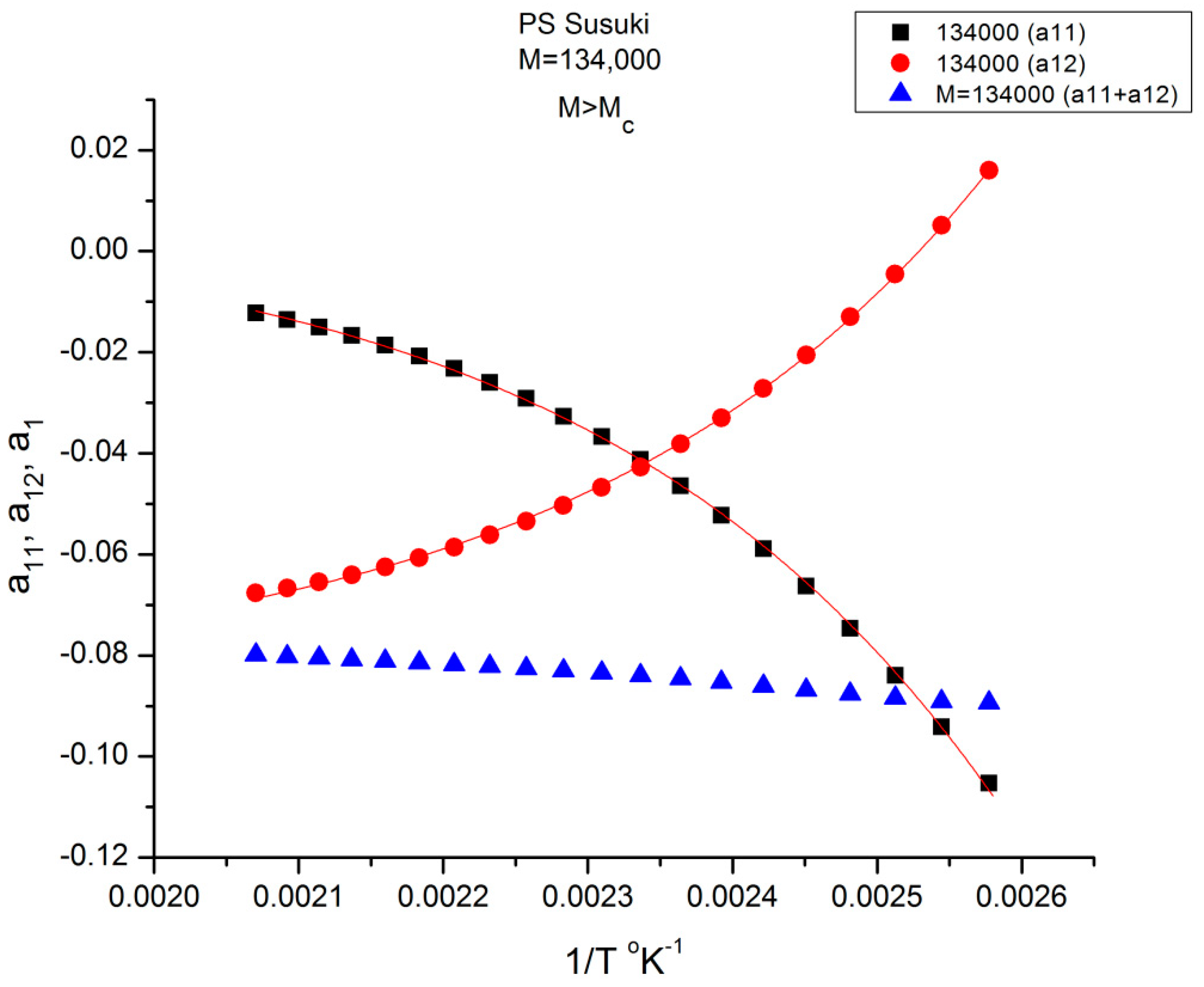
Figure 9 is a plot of the values of a₁₁(T) and a₁₂(T) found by regression for M = 134,000 according to Equations (6) and (7). The black squares represent a₁₁, and the red dots represent a₁₂. The blue triangles refer to their sum a₁(T) = a₁₁(T)+ a₁₂(T) in Equation (6). The validation test of the separation of M and T consists in determining whether the sum a₁ = a₁₁+ a₁₂ of Equation (6) remains constant when 1/T varies (and the blue triangles remain horizontally aligned) for this particular value of M. Figure 9 shows that the horizontality of a₁ is never realized for M = 134,000 since a₁(M) slightly varies with T. The slope is closer to 0 in the higher T region (the lower 1/T values). The separation of M and T is invalidated for this molecular weight (134,000 g/mole). We repeat the same test in Figure 9 for all the other M values available. For certain discrete values of M, e.g., 2M_c, 4M_c, 8M_c, etc. the line of blue triangles remains strictly horizontal when T varies: a₁(M,T) = a₁(M) for those discrete values of M. For the other values of M, a “structure of a₁(M) appears visible, fragmenting a₁₁(M,T) and a₁₂(M,T) into ranges of sequential M, for which compensations occur. It appears that the compensation points always coincide with the values of M for which the blue lines are horizontal. Depending on the configuration status of our assumptions in Equation (7), some period doubling compensation may be missing (e.g., 16M_c for configuration (1,0) [8]).

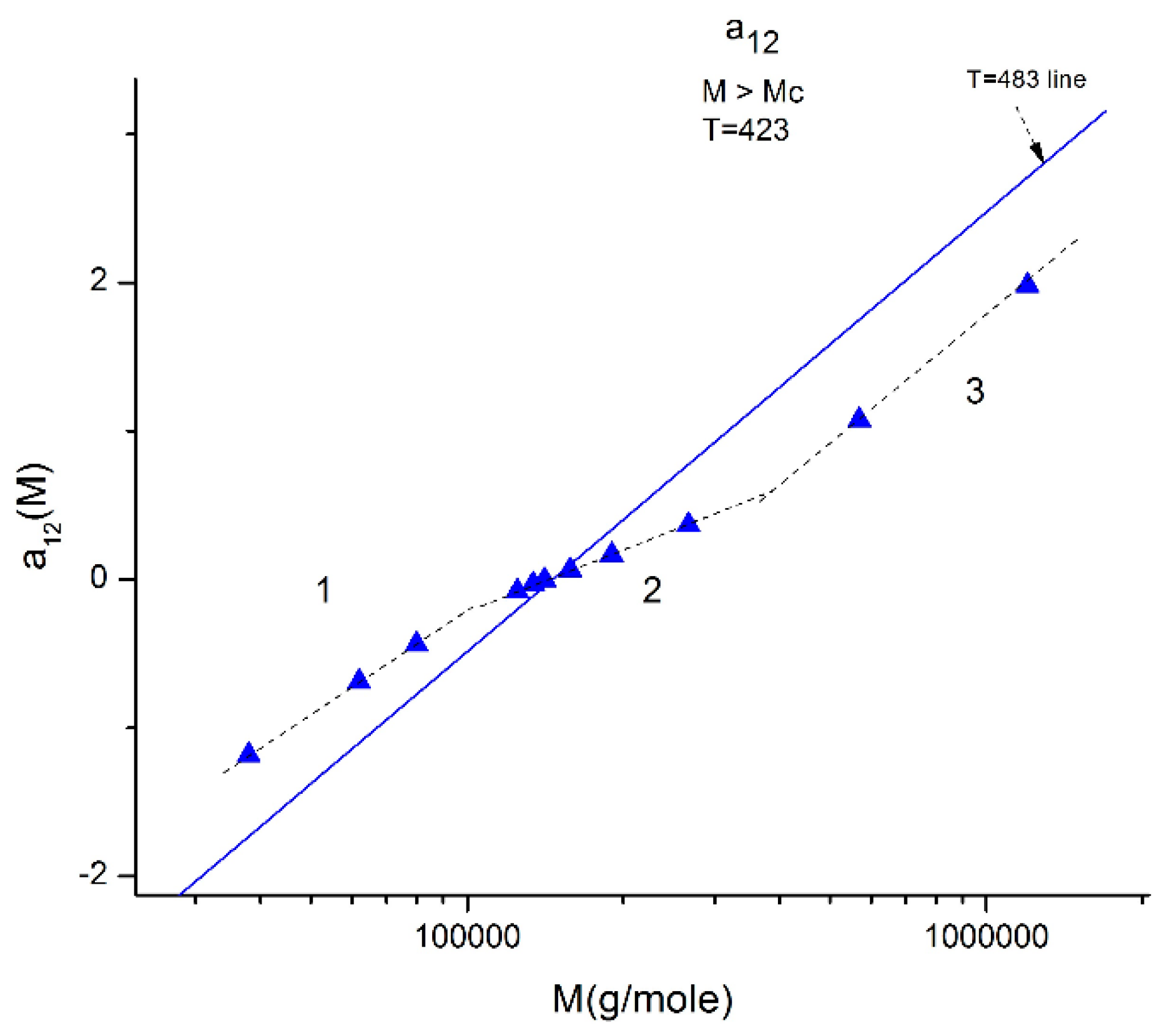
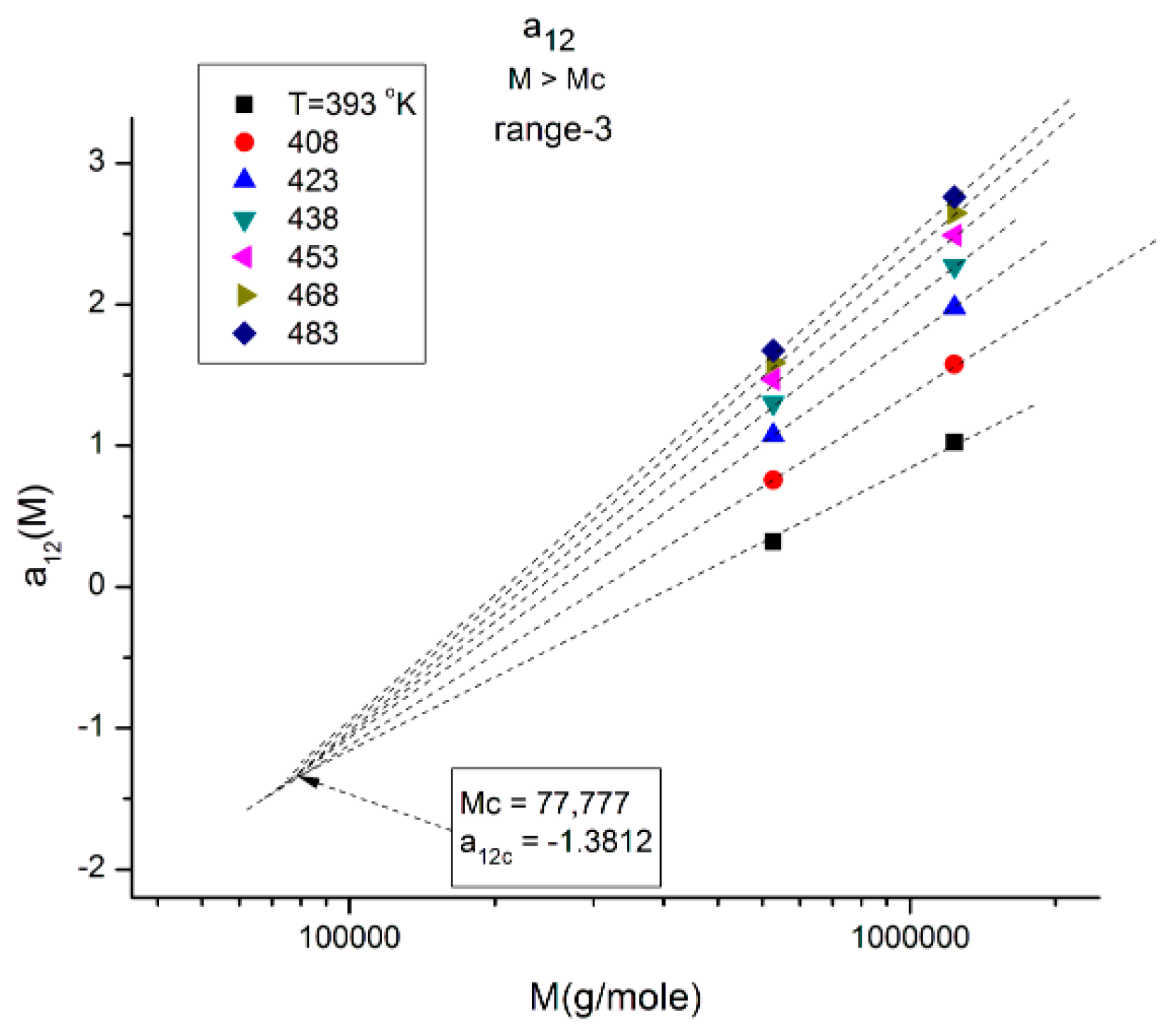
We illustrate these observations in Figure 10, Figure 11, Figure 12, Figure 13 and Figure 14 by plotting a₁₂(M) vs. log M for three fragmented ranges of M,T values. Figure 10 shows the separation of the molecular weight range in three sub-ranges, all above M_c, for a₁₂(M) at T = 423 K (150 °C).

Figure 10. Plot of a₁₂(M) at constant T (T = 423 °K is represented by the blue triangles) delimitating 3 ranges: 1, 2, 3. When T varies, the three ranges still exist, but the respective disposition of the three segments is different. The straight line corresponds to T = 483 °K for which the three ranges almost fuse into a single one (range-2 points) is slightly above the straight line yet parallel to it. The T = 423 and T = 483 lines, and the lines for the other T, all cross at a universal “pole R” corresponding to M = 4M_c and a₁₂ = a₁₁ = 0 whatever T.

Figure 10. Plot of a₁₂(M) at constant T (T = 423 °K is represented by the blue triangles) delimitating 3 ranges: 1, 2, 3. When T varies, the three ranges still exist, but the respective disposition of the three segments is different. The straight line corresponds to T = 483 °K for which the three ranges almost fuse into a single one (range-2 points) is slightly above the straight line yet parallel to it. The T = 423 and T = 483 lines, and the lines for the other T, all cross at a universal “pole R” corresponding to M = 4M_c and a₁₂ = a₁₁ = 0 whatever T.

In Figure 11, the values of a₁₂(M,T). for M_c < M < 2M_c) (i.e., in “range-1”), at various T form a collection of straight lines compensating at M = 188,000 ~5M_c when M is plotted on a log scale. The y-coordinate of the compensation point is positive. The lines compensate as T increases from 120 °C to 210 °C. The slope of a₁₂ (T) vs. log M reaches an asymptotic value in the higher T region, which lines up this range-1 of data with the data located in the other ranges, range 2 and range-3, at higher M (Figure 12 and Figure 13).

Figure 11. Same figure as Figure 10 restricted to the “range-1” M values and various T. The isothermal segments of a₁₂(M) of range-1 all compensate as T increases. The slope reaches an asymptotic limit for T > 453 °K (approximately).

Figure 11. Same figure as Figure 10 restricted to the “range-1” M values and various T. The isothermal segments of a₁₂(M) of range-1 all compensate as T increases. The slope reaches an asymptotic limit for T > 453 °K (approximately).

Figure 12. This figure explores range-2 of Figure 10 at various T indicated by the different symbols. There is a double-compensation point at the pole M_R~4M_c delimitating two ranges 2L and 2R The value of a₁₂ at the compensation point is zero, which also occurs for a₁₁(M) vs. log M (not shown). This figure should be compared to Figure 11 and Figure 13.

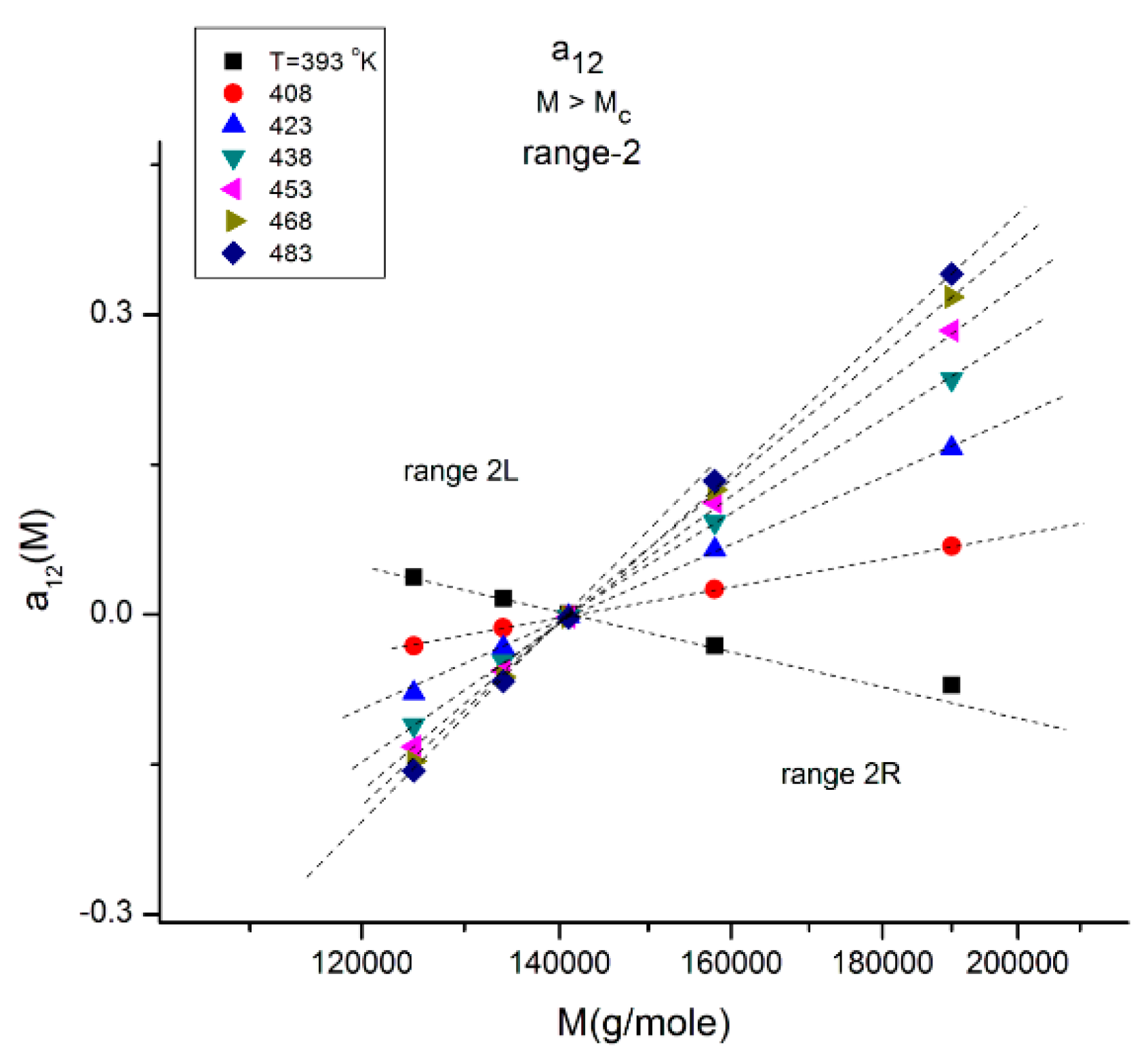
Figure 12. This figure explores range-2 of Figure 10 at various T indicated by the different symbols. There is a double-compensation point at the pole M_R~4M_c delimitating two ranges 2L and 2R The value of a₁₂ at the compensation point is zero, which also occurs for a₁₁(M) vs. log M (not shown). This figure should be compared to Figure 11 and Figure 13.

Figure 12 explores “range-2” of the values of the molecular weight, showing a compensation point at M = M_R = 144,000 ~ 4M_c. The value of a₁₂ at the compensation point is zero, which is also the case for a₁₁ (not shown), indicating that a₁ = a₁₁ + a₁₂ = 0 is a special solution for the separation of M and T corresponding to a₁₁ = a₁₂ = 0. In Figure 12 we see that in range-2 (M < M_R), the compensation lines converge to the compensation point, whereas they emerge from the compensation point in range 2R (M > M_R).

Figure 13. Same as in Figure 10, with a₁₂(M,T) now focusing on range 3 and showing a negative compensation point at M~2M_c. Note the y-coordinate value of the compensation point to be compared with that of the compensation point in range 1 (Figure 11): their sum equals −1.

Figure 13. Same as in Figure 10, with a₁₂(M,T) now focusing on range 3 and showing a negative compensation point at M~2M_c. Note the y-coordinate value of the compensation point to be compared with that of the compensation point in range 1 (Figure 11): their sum equals −1.

In Figure 13, the a₁₂(T,M) values of M are located in range-3, and when T varies, the isotherms compensate at M~2M_c with a negative value of the y-coordinate of the compensation point. Interestingly, if one compares the three ranges in Figure 11, Figure 12 and Figure 13, the higher M range (range-3 in Figure 13) corresponds to a “negative” compensation; that is, the isotherms emerge from a lower M value, while the compensation is “positive” in range-1 (Figure 11), i.e., the isotherms converge to a higher M value. The situation in range-2 is intermediate with the combination of a positive and a negative compensation using the same compensation point at M = M_R. The description of a₁₂(M,T) can thus be described as a succession of positive and negative compensations, a very interesting network structure threaded by the interdependence of the effect of M and T on viscosity. Also noticeable are the complementarities of the y-coordinate values of the compensations for Figure 11 and Figure 13, which add up to −1.

The variation of a₁₁(M,T) is similar to a₁₂(M,T) for the effect of M at T constant, yet almost symmetrically “opposite” to a₁₂(M,T) for the effect of T at M constant. In Figure 14, Figure 15 and Figure 16, a₁₁ and a₁₂ are plotted against log M at T constant, showing two temperatures only: a low T = 403 °K (130 °C) and a high T = 478 °K (205 °C).

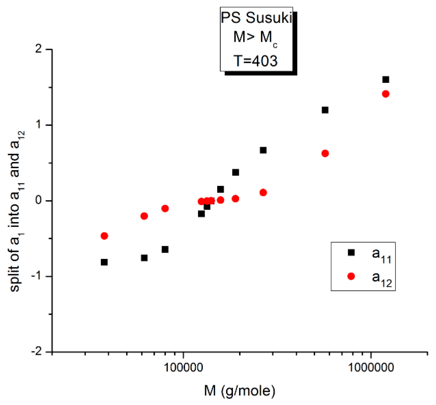
Figure 14. Comparing a₁₁(M) and a₁₂(M) for T = 403 °K. The a₁₂(M) values (red dots) have already been presented in Figure 10, fragmenting the M range into three sub-ranges. The two structural components of a₁ cross at the pole (M = M_R), where they become 0.

Figure 14. Comparing a₁₁(M) and a₁₂(M) for T = 403 °K. The a₁₂(M) values (red dots) have already been presented in Figure 10, fragmenting the M range into three sub-ranges. The two structural components of a₁ cross at the pole (M = M_R), where they become 0.

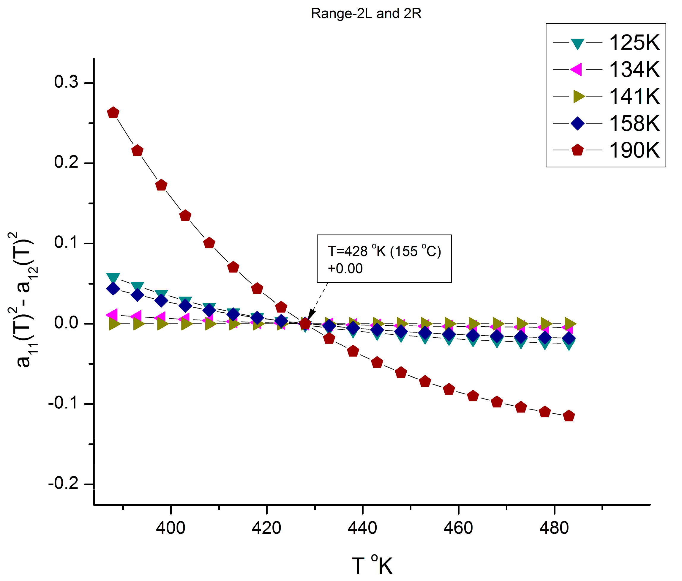
We see in Figure 14, for this low T value (T = 403 °K), the appearance of symmetry for a₁₁(M) and a₁₂(M) around their mean value, but in reality, for such low temperatures up to T = 448 °K, the axis of symmetry is different for the values of M superior or inferior to M_R = 4M_c(at M_R, both a₁₁and a₁₂ are equal to 0, as we saw in Figure 12). Data points are missing at both extremities of the plot to confirm the possibility for a₁₁(M) and a₁₂(M) to cross on the symmetry lines at M ~ M_c and M~55.5 M_c, confirming the presence of periodic anchors for discrete M values.

Figure 15. Split of a₁ into a₁₁(M) and a₁₂(M) at higher T, 478 K, in this graph. The average value, a₁/2, represented by the dotted line, appears to be the symmetrical axis of the data, the same across the pole M_R. The green triangles display the behavior of a₁(M) vs. log M, which can be fitted by a straight line with slope ~ 3.4, the classical result.

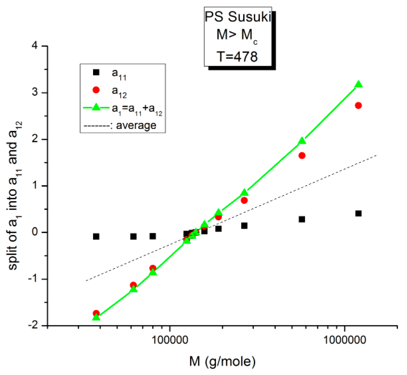
Figure 15. Split of a₁ into a₁₁(M) and a₁₂(M) at higher T, 478 K, in this graph. The average value, a₁/2, represented by the dotted line, appears to be the symmetrical axis of the data, the same across the pole M_R. The green triangles display the behavior of a₁(M) vs. log M, which can be fitted by a straight line with slope ~ 3.4, the classical result.

Figure 15 displays the equivalent of Figure 14 at a higher temperature: T = 478 K (205 °C). Like at lower T, a₁₁(M) and a₁₂(M) cross at M_R = 4M_c, but the disposition of the red dots (a₁₂) and of the black squares (a₁₁) on the graph looks different than at lower temperatures. This implies that the influence of T on the interdependence of M and T is not the same in the three sub-ranges of M, range-1, 2, or 3. Likewise, the influence of M on the interdependency of T and M is not the same in the three temperature sub-ranges 1, 2, or 3, delimited by T_g, T_g + 23 °C and T_LL (see the discussion). The green triangles represent a₁(M) = a₁₁(M) + a₁₂(M) vs. log M (i.e., a plot of log μ_o vs. log M pursuant to Equation (6)). These points can be fitted by a straight line across M_R (r² = 0.9983) with slope = 3.372, which is the classical exponent value characteristic of PS melts. This is expected since we used data generated by the classical formula (Equations (3–(5)). One sees that a two-phase formulation of the viscosity, Equations (6) and (7), that assumes viscosity to be the product of two terms for which the effect of M and T are not separable, provides the same value of the slope for log μ_o vs. log M for M > M_c than in the classical view, that assumes that the effect of M and T on the viscosity separates (Figure 1). This apparent paradox proves, at least, that the veracity of the features in Figure 1 does not uniquely imply the separation of M and T in the viscosity. On the contrary, Figure 10, Figure 11, Figure 12, Figure 13 and Figure 14 demonstrate the particularities of the dependence of the effect of T and M on the viscosity in ways that cannot be deducted if M and T were separable. In particular, among the special features of the dependence between M and T is the finding of a special molecular weight M_R = 4 M_c. Figure 15 shows the average value of a₁₁(M) and a₁₂(M), a₁/2, represented by the dotted line, which appears to be the symmetrical axis across this M_R value. This “pole” molecular weight, a clear marker of the dual-phase viscosity formulation in range M > M_c, is not M_c itself but 4M_c, a value of M that does not resonate to be significant in the classical paradigm. Likewise for the T scale in the T > T_g range, as we further explain in the Discussion section, the T_LL transition [11,12] has no physical reason to exist in the classical theories of melt viscoelasticity and is vehemently described as an artifact by the adepts of the classical views [12], yet erroneously so, in our opinion, since this temperature determines the success or the failure of a new processing benefit for the polymer resins industry: “sustained orientation” [4,7].

Figure 16. This figure is the same as Figure 15, focusing on different aspects. First, the linearity of the variation of a₁₁(M) and a₁₂(M) vs. log M for M > M_c at higher T and second, the possible significance of the slope of the two “phases” generated by Equations (6) and (7) when plotted against log M.

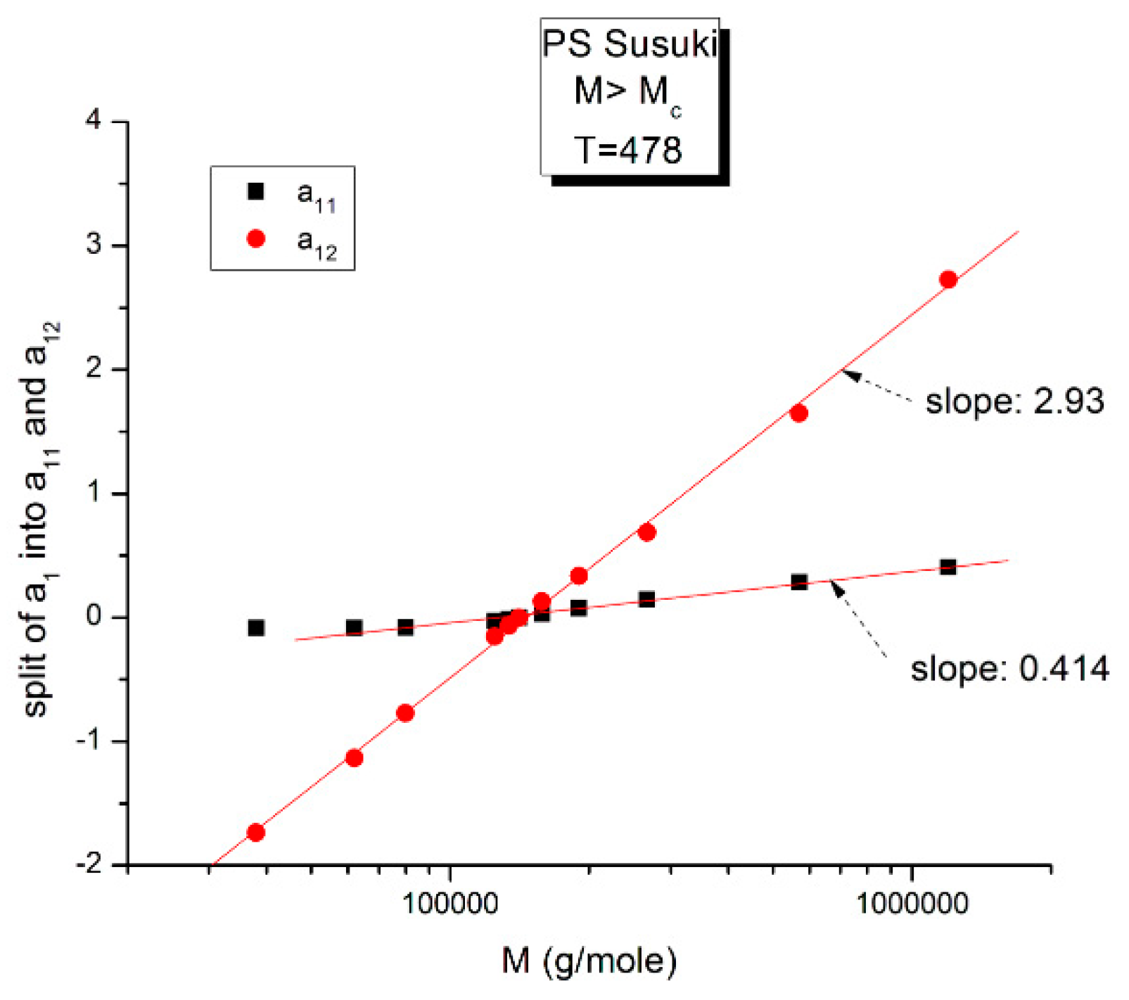
Figure 16. This figure is the same as Figure 15, focusing on different aspects. First, the linearity of the variation of a₁₁(M) and a₁₂(M) vs. log M for M > M_c at higher T and second, the possible significance of the slope of the two “phases” generated by Equations (6) and (7) when plotted against log M.

Figure 16 may possibly be the simplest explanation of the classically acclaimed formulation of viscosity by Equation (5) for M > M_c. A Dual-Phase interpretation of the classically acclaimed 3.4 exponent is that 3.4 = (3 + 0.4) and that one should separate the understanding of the exponent 3 from the exponent 0.4, instead of trying to modify the explanation of the exponent 3 (say by de Gennes [5]) by incorporation of additional mechanisms such as contour length fluctuation, constraint release and chain stretching (Chapter 7 of [7]) to reach the value of 3.4 for the exponent. A Dual-Phase explanation is the separation of the phases in the viscosity equation instead of the separation of the effect of M and T.

Figure 16 is the same as Figure 15 plotted differently, showing different aspects of this graph: the variation of a₁₁(M), the black squares with slope 0.414, and of a₁₂(M), the red dots with slope ~3 at high T. The difference between the lower temperature range of the melt (e.g., in Figure 10) and the higher temperature range (Figure 16) is now clearer: the lines in Figure 16 represent the log μ_o1(M), and the log μ_o2(M) vs. log M viscosity plots of the two-phases 1 and 2 at T = 478 °K, and these lines are straight all across and not fragmented segments as they appear at lower T (403 °K in Figure 15). This, again, clearly reveals not only the separate and distinct role of M and T on the viscosity but also their compensating interactive effects.

Speaking in terms of viscosity, Figure 16 represents the molecular weight dependence of the log of viscosity of “phase 1 and phase 2” pursuant to the “Dual-Phase equations”, Equations (6) and (7): it provides the dual-structure of log μ_o into two terms, log μ_o1, represented by the black squares for a₁₁(M) with slope 0.414 (phase 1) and log μ_o2, the red dots for a₁₂(M), with slope 2.93 (phase 2). Note that if we change the temperature from T = 478 °K to T = 483 °K, the respective slopes of the lines in Figure 16 become 0.328 and 3.0 for the respective phases, giving a total exponent of 3.328 for the variation of a₁(M) = log μ_o(M) in Equation (7). It is, indeed, remarkable to find for the slope of phase 2, the “core-phase”, the value of 3, which is the value found by de Gennes in the original reptation calculation of the molecular weight dependence of the Newtonian viscosity [6] and to attribute to phase 1 “the entanglement phase” the “corrective” additional 0.4 exponent value classically assigned to sophisticated perfections of the original de Gennes’ tube calculations (see Figure 16 caption).

Figure 17. This plot (for M > M_c) shows the average value between a₁₁(T) and a₁₂ (T), which is half the value of a₁ (T) = log μ_o(T), plotted against log M. For M > 2M_c (~77,000), a single straight line goes through the data, which renders μ_o(T) independent of T: T and M separate. Below 2M_c, we observe a compensation of lines as T varies instead of the unique straight line: T and M no longer separate.

Figure 17. This plot (for M > M_c) shows the average value between a₁₁(T) and a₁₂ (T), which is half the value of a₁ (T) = log μ_o(T), plotted against log M. For M > 2M_c (~77,000), a single straight line goes through the data, which renders μ_o(T) independent of T: T and M separate. Below 2M_c, we observe a compensation of lines as T varies instead of the unique straight line: T and M no longer separate.

Figure 17 illustrates how the separation of M and T for M > 2M_c is simply the result of an illusion created by the use of log axes that compresses the resolution of a significant residual periodically fluctuating around 0. This figure plots half the value of log μ_o = a₁ against log M for all the T values available (T = 393–483 °K). We observe that a₁(M)/2 = (a₁₁ + a₁₂)/2 varies with T and M in the lower molecular weight range (M_c < M <2M_c), but that in other ranges of M (M > 2M_c) there is a single straight line with all the points superposing; that is, it apparently looks temperature independent, varying only with M; the effect of M and T appears to separate in the expression of the total viscosity for M > 2M_c. In this region of M and T, the slope of a₁ vs. log M is 2 * 1.686 = 3.372, the expected value from the classical model of viscosity. Below M = 2 M_c, however, we observe a spectrum of compensating lines as T varies, the visible proof using these axes that T and M at least do not separate in this range. The details for M < 2M_cis blown up in Figure 18a, and the compensation search is shown in Figure 18b. We can clearly see that the slope of each isotherm increases with T up to T ~ 428–448 °K (155–175 °C) and that for T beyond that temperature, the slope asymptotically converges to a value close to (but not equal to) the 3.372 slope of the T independent region (Chapter 4 of [8]).

In range-2 and 3 for M, the a₁₁(T) and a₁₂(T) are more symmetrically disposed with respect to their average value when M varies, especially at high temperatures (e.g., Figure 15), and therefore their half sum gives the illusion to lie more closely on the average value line, giving the appearance of being independent of T. However, if we zoom on the points of the M > 2M_c region in Figure 17 or if we analyze the residuals of their linear regression, the illusion of the separation of T and M reveals itself unequivocally (see Figure 12 and Figure 13).

Figure 18. (a) Compensation of the isothermal segments for the average of a₁₁(M) and a₁₂(M) in range-1 (M < 2M_c). The compensation Search is displayed in (b). (b) Compensation search to determine the compensation point coordinates in Figure 18a; the coordinates are calculated from the slope and intercept of the compensation line in this plot: intercept:−0.4679; slope: −4.89022. The value of M at the compensation point is, therefore, 10^4.89022 = 77,664, and the y-coordinate is −0.4679.

Figure 18. (a) Compensation of the isothermal segments for the average of a₁₁(M) and a₁₂(M) in range-1 (M < 2M_c). The compensation Search is displayed in (b). (b) Compensation search to determine the compensation point coordinates in Figure 18a; the coordinates are calculated from the slope and intercept of the compensation line in this plot: intercept:−0.4679; slope: −4.89022. The value of M at the compensation point is, therefore, 10^4.89022 = 77,664, and the y-coordinate is −0.4679.

Another interesting observation consists of comparing the compensation coordinates for the a₁(M,T) data in range-1 (Figure 18a) and for the a₁₂(M,T) data in range-3 (Figure 13): they have the same value of M at the compensation but their y-coordinates are shifted by approximately 1, a clear indication that the fragmentation of the T range and the M range for T > T_g and M > M_c, respectively, are dependent and coupled in the expression of the viscosity of polymer melts, an important conclusion totally missed by the current paradigm of rheology.

In summary, the regression of the Newtonian viscosity data as a function of T and M by Equations (6) and (7) show that b₂ and b₄ become simultaneously zero for periodic values of M, which are multiples of M_c (33,000 to 36,000 g/mole), pursuant to period doubling: 2M_c, 4M_c, 8M_c, 16M_c. For all other values of M, the values of b₂ and b₄ are quite small but not zero, yet small enough to make the sum (b₂exp(ΔH_2R/T) + b₄exp(ΔH₂/T)) give the appearance that the separation of the variables is justified, although it is not. Furthermore, we observe that the sum (b₂exp(ΔH_2R/T) + b₄exp(ΔH₂/T)), although small, structures with M in a way that makes the periodic molecular weights for the zeros the compensation points for the other M values when M is expressed as log M (see the Discussion at Figure 19 for a visual summary). As we mentioned at the onset of section B, our current presentation of the periodic dependence of T and M in the expression of the viscosity has been simplified in this paper. A more complete and thorough mathematical proof will be provided separately [8]. The key result of this section B is the understanding that all current models of melt viscoelasticity of polymers based on the separation of M and T are approximations that overly simplify the effect of M and T, miss out some fundamental aspects of the interactive coupling between T and M, and are, as proven mathematically, incorrectly describing the interactions in polymers, theoretically speaking. Of course, it should also be added that the separation of T and M becomes a better approximation at higher melt temperature and for M > 2M_c (Figure 17), which are the usual ranges of use of polymer resins, a choice that may explain why the previous models [4,8] remained falsely convinced of the true separation of T and M, despite of the contrary in reality.

3. Discussion

To summarize the results presented in sections A and B, we conclude that Figure 1, representing the concepts of the current paradigm of rheology, is incomplete and misleads the comprehension of the flow of melts because it is too simplistic; it does not correctly describe the effect of temperature, T, or the effect of the molecular weight, M, and misses out the consequences of their coupling on the fragmentation of rheological ranges affecting the Newtonian viscosity; in many ways its shortcomings become inconsistencies leading to false interpretations. For instance, the classical interpretation of the viscosity break at M_c as the proof for entanglements (Figure 1) appears to be directly challenged by the work presented in this communication (Figure 2, Figure 3, Figure 4, Figure 5, Figure 6 and Figure 7). The failure of the classical interpretation of entanglements has been reported and documented by us before [4,7,18], showing its negative impact on the polymer processing industry [4,7]. This paper makes use of mathematical tools developed from ideas inspired by the dual and cross-dual aspects of the rheology of polymer melts [7,8,9] to reveal fundamental inconsistencies in the current assumptions leading to the classical understanding of the rheology of polymer melts [10].

In section A, the graphs in Figure 1, Figure 2, Figure 3, Figure 4, Figure 5, Figure 6 and Figure 7 encompass the M < M_c and M > M_c regions to evaluate the classical view assumption that the entanglement molecular weight is defined at the crossing of the distinct behaviors below and above M_c. Figure 1 schematizes the break at M_c that is supposed to be independent of T. In the other graphs, in Figure 2, Figure 3, Figure 4, Figure 5 and Figure 6, the change of color for the squares, from red at high M to black at lower M, starts at the value of M_c projected for PS: 33,000 to 36,000 g/mole [1]. The highest T is in Figure 7 (T = infinity), followed by, in descending order, Figure 2, Figure 3, Figure 4, Figure 5 and Figure 6. Figure 7 is the only graph resembling Figure 1: 2 straight lines and a sharp break at M_c, accepting the reservations we made for the 1.51 slope for M < M_c (instead of 1) and the higher value of M_c at the break than the quoted values in the literature (48,000 instead of 36,000). Only Figure 2 (at T = 210 °C) could validate with a certain certitude the classical view for M_c and above M_c, yet needed the reserves we made for the description of the M < M_c distinct curvature from the expected straight line one in Figure 1. M_c is at its correct literature value in Figure 2. As T decreases, from Figure 3 to 6, the overall aspect of the graph starts to systematically diverge from the classical expected view of Figure 1, displaying three straight lines (not two) in Figure 3 and Figure 4, along with two molecular breaks, M_c and M’_c, not just M_c; and then, only two straight lines with a break at M’_c and no break at M_c for the two lowest T (Figure 5 and Figure 6). For instance, in Figure 5 (T = 125 °C), there is no break at the change of color from red to black at M_c, and the straight line passing through the “entangled melt” continues unbroken down to M’_c = M_c/8. Is the entanglement molecular weight now defined by M’_c = M_c/8? Do we need to define another criterion than the break of the molecular weight in a graph like Figure 1 to characterize M_c? This is the first fundamental challenge raised in this paper to the current paradigm of rheology. Along with it, what is the physical significance of the M_c/8 molecular weight?

The second fundamental question raised concerns the separation of the effect of M and T in the formulation of the viscosity. This question already surfaces in Figure 8, at the end of section A, by showing that the molecular weight exponent for the Newtonian viscosity, the famous 3.4 slope in Figure 1 for M > M_c, explained with great details by the reptation school [6], seemingly varies systematically with temperature, which would contradict the separation of T and M if it were confirmed. Section B presents a simplified version of a mathematical proof that we have developed [8] to evaluate the classical assumption of the separation of T and M in the formulation of viscosity. The overall conclusion is that the separation of T and M in the expression of viscosity is invalid except for a series of specific molecular weight values that are multiples of M_c: 2M_c, 4M_c, 8M_c, 16M_c, etc. We found that the value of M_R = 4M_c holds a special role among all the solutions, the role of a “pole reference” for the melt (a₁₁ = a₁₂ = a₁ = 0), symbolized by the presence of the subscript “R” in some of the terms in Equation (7). In other words, we discovered in section A the existence of a certain special molecular weight M’_c = M_c/8, and in section B the existence of another special molecular weight, M_R = 4 M_c, possibly indicating that the period doubling observed above M_c could actually start at M’_c? Note that playing along with this period doubling picture, the value of M_e of the rubber elasticity theory falls right between M’_c and M_c with M_e = M_c/2 = 4 M’_c. Figure 19 summarizes the period doubling fragmentation of the M range at various values of T pursuant to “configuration (0,1)”. Figure 9, Figure 10, Figure 11, Figure 12, Figure 13, Figure 14, Figure 15, Figure 16, Figure 17 and Figure 18a,b above referred to configuration (0,0), the simplest to describe. The difference between the configurations bears on the complexity and the status of certain constants to be found by regression, which results in certain solutions being skipped for period doubling: for instance, 16M_c is not a solution for configuration (1,0). These complications are not essential for this introductory presentation.

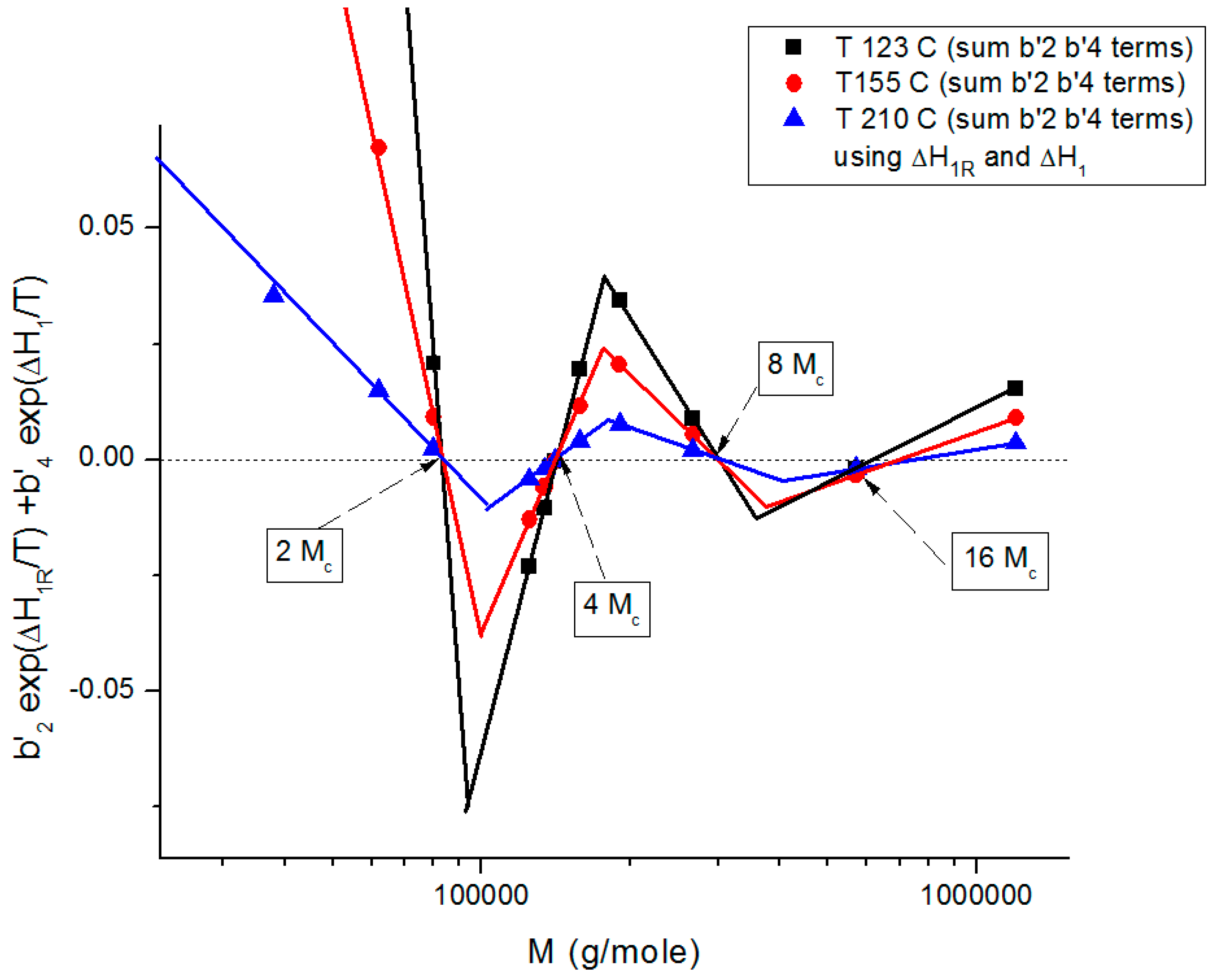
Figure 19 shows the sum of the b’₂ and the b’₄ terms in Equation (7), configuration (0,1)), plotted against log M. This graph summarizes the various facets of the sophistication of the coupling between the T and M variables introduced in the previous figures (Figure 9, Figure 10, Figure 11, Figure 12, Figure 13, Figure 14, Figure 15, Figure 16, Figure 17 and Figure 18b): it shows the true values of the zeros (b’₂ = b’₄ = 0) corresponding to the compensation of the non-zero regions, it shows the fragmentation of M in three regions and the period doubling of M_c. The low value of the sum of the b’₂ and b’₄ terms in Figure 19 explains the visual illusion of the separation of M and T perceived in Figure 17. Also, the sum of the b’₂ and b’₄ terms becomes smaller for M > 2M_c and as T increases, making the separation of T and M appear more real.

Figure 19. Proposed structuration by the coupling of T and M towards variable separation, which occurs at M = 2M_c, 4M_c, 8M_c, 16M_c for configuration (0,1) in Equation (7). This figure shows the alignment of the data points on straight lines, their compensations occurring on the zero horizontal line and the systematic departure from the criteria for the separation of M and T whose amplitude gets smaller as M increases (M > 2M_c), explaining the appearance of the M and T separation more real at higher M values. See [8] for details.

Figure 19. Proposed structuration by the coupling of T and M towards variable separation, which occurs at M = 2M_c, 4M_c, 8M_c, 16M_c for configuration (0,1) in Equation (7). This figure shows the alignment of the data points on straight lines, their compensations occurring on the zero horizontal line and the systematic departure from the criteria for the separation of M and T whose amplitude gets smaller as M increases (M > 2M_c), explaining the appearance of the M and T separation more real at higher M values. See [8] for details.

We mentioned in several instances of this presentation and in previous publications [7,10] the need to fragment the melt temperature range in 3 rheological ranges for T > T_g, in a way similar to the fragmentation in three rheological ranges of the M molecular range in Figure 10, Figure 11, Figure 12, Figure 13 and Figure 19: M’_c < M < M_c, M_c < M < M_R, and M > M_R. The fragmentation of the temperature delimitates T_g < T < T_g + 23 °C, T_g + 23 < T < T_LL, and T > T_LL where T_LL is the liquid-liquid temperature associated with the Dual-Phase model’s dissipative transition temperature [4,7,8,9,10,11,12]. T_LL varies with M [11] but takes values between 155 to 175 °C for PS. T_g is also variable with M below M_c reaching an asymptote in the M > M_c range so that the value of T_g + 23 °C for M > M_c stabilizes around 125 °C. [10]. Figure 20 and Figure 21 give a possible explanation for the temperature fragmentation of the melt above T_g using the mathematical framework of Equations (6) and (7).

Figure 20 and Figure 21 show the same plot (which could have been combined in one graph, yet they are split for clarity to show their different poles for selected different values of M). Figure 20 only has the selected group of M values shown in the insert that belong to either range-1 or range-3, but none of range-2 of the molecular weight fragmentation. The other values of M giving the alternative pole are shown in Figure 21. All the curves in Figure 20 compensate at T ~ T_g + 23 °C., and all the curves in Figure 21 compensate at T ~ T_LL. Note: in the insert, 38K refers to M = 38,000, etc.

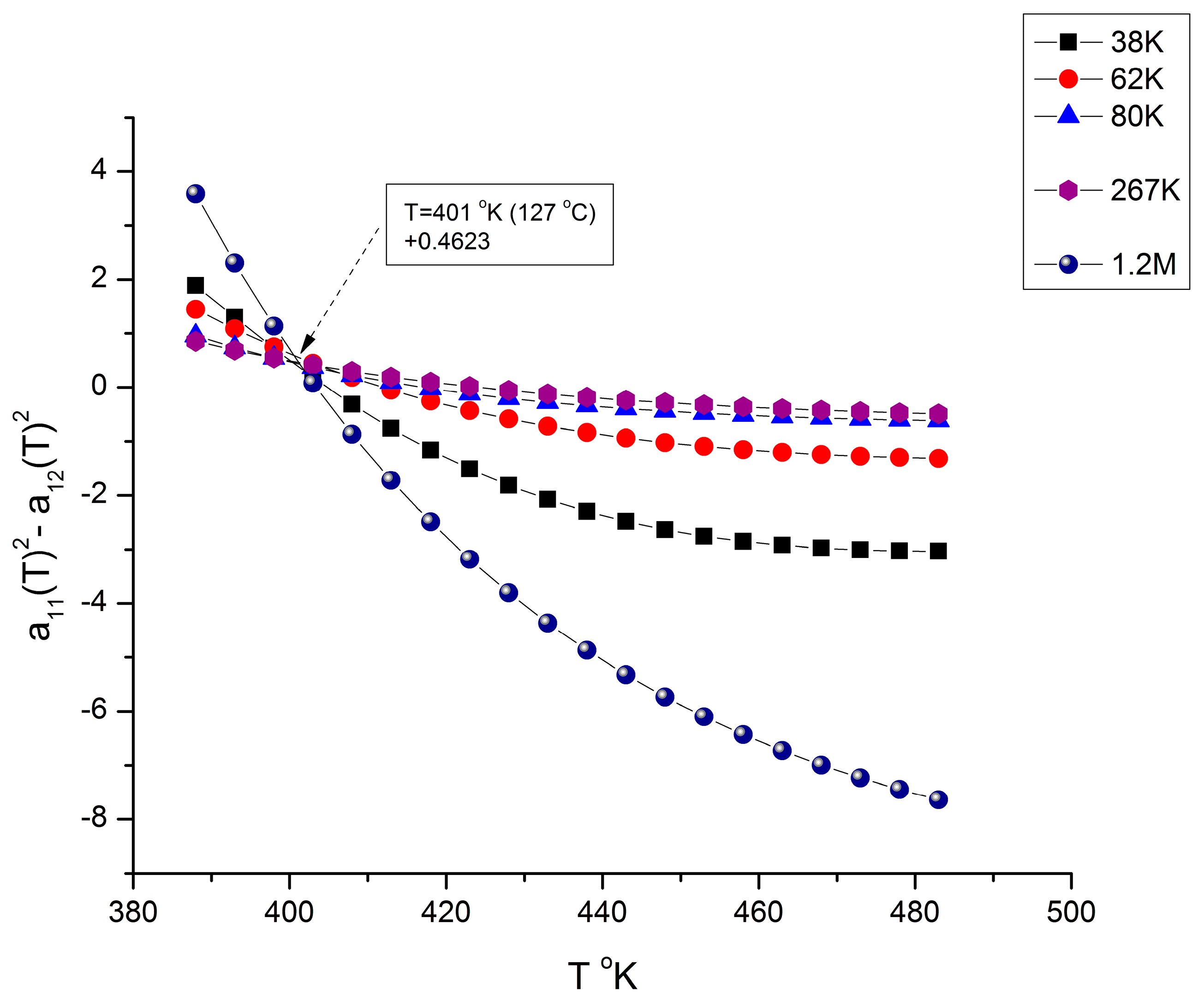
Both Figure 20 and Figure 21 are plots of (a₁₁² − a₁₂²) vs. T for various values of M remaining constant when T varies. In a certain sense, these figures are similar to Figure 11, Figure 12 and Figure 13, which displayed the fragmentation of the M range in three sub-ranges. Figure 20 and Figure 21, however, use a slightly different y-coordinate, and the role of M and T is reversed: T varies, and M is constant in Figure 20 and Figure 21, whereas M varies and T is constant in Figure 11, Figure 12 and Figure 13. Yet the presence of poles (compensations) is visible when T is scanned from T_g to 210 °C. In Figure 20, the curves compensate at T = 401 °K (127 °C), but only for a discrete set of M values listed, not for all the values of M (the other values of M are in Figure 21); additionally, the compensation y-coordinate in Figure 20 is not 0, but 0.4623. Figure 21 applies to all the M values not listed in Figure 20 (i.e., for M = 125,000 to 190,000), and it is shown that the curves compensate at a different temperature, T = 428 °K (155 °C), and on the y-coordinate axis (a₁₁ = a₁₂ = 0). The values found for the two compensations, 127 °C and 155 °C in Figure 20 and Figure 21, respectively, appear to match the value given for T_g + 23 °C and T_LL from other estimation sources [9,10,11,12]. In other words, the fragmentation of the temperature and of the molecular weight ranges into rheological sub-ranges is due to the interactive coupling between the effect of M and T in the definition of the viscosity (shown as an example in Equations (6) and (7)).

Figure 20 and Figure 21 reveal an added complexity, which is absent in Figure 11, Figure 12 and Figure 13: whether the curves, for any given value of M, belong to either the pole group in Figure 20 or Figure 21. This complexity in the inter-coupling between M and T, and of its incidence on the fragmentation, has been eluded to earlier when we noted that the existence of pole 16M_c was part of the period-doubling solutions for configuration (0, 1) in Figure 19, but not for configuration (1,0). This shows that the rheology of the coupling μ_o(M,T) is, indeed, more sophisticated than what has been introduced in this communication and needs more elaboration [8].

Let us now provide a short presentation of the differences between our challenging model of polymer physics to explain the rheology of polymer melts and the classical molecular dynamic models of rheology currently admitted as the current paradigm. The reader should refer to the Preamble of [7,18] as well as [4] for a brief presentation of the theoretical background of our new model of interactive dissipative coupling applied to polymers [7,18] and of its practical application to “disentangle” polymer melts during processing to temporarily decrease their viscosity during processing [4]. These three references are fully available from the ResearchGate archive platform (“Preamble: Introduction to the Dual-Phase Model of Polymer Interactions and to the Cross-Dual-Phase Model of Entanglements”).

The present understanding of the physics of macromolecules is based on an analysis of the properties of a single chain. The presence of the other chains is perceived as a mean field influence on the properties of that chain. The reptation model of de Gennes [6] considers that “entanglements” arise at M_c when the homogeneous field, creating the environment of the chains, is modified due to the higher molecular weight of the macromolecules to include obstacles restricting the motion of the single chain. In other words, topological constraints occurring for higher molecular weights chain lengths create the obstacles that explain the rise of the viscosity at M_c compared to the viscosity in the absence of such obstacles, which has been modelized by Rouse [5]. For the classical view of rheology, the relaxation time of the molecular motions occurring within the chain, in the presence or not of the topological constraints, generates the stresses and strains when the fluid is submitted to a strain rate tensor to put it in motion. The challenge is to correlate the relaxation times obtained from the analysis of the rheological parameters, for example, from the Newtonian viscosity or the cross-over relaxation time to the relaxation times calculated from the conformation and configuration description of the polymer chain.

In conclusion, to briefly summarize the foundation of the classical dynamic models of rheology [5,6], their statistical system is the macromolecule, and the chain dynamic is described by the chain relaxation time (Rouse or reptation time).

For the Dual-conformers approach, the statistical system studied to define the stresses and the strains is not a single chain, and the molecular motions are not apprehended by their relaxation times. We refer to a basic unit of deformation within the chain, the Dual-conformer, and consider the properties of a statistical system consisting of several Dual-conformers belonging to the same macromolecule but also to other macromolecules, all submitted to the constraints of a statistical model, the Grain-Field Statistics Theory, that defines their evolving interactive coupling as an open dissipative system [4,7,18]. The assumptions of the model define mathematically what “evolving interactive coupling” means when the full collection of Dual-conformers is brought out of equilibrium by an outside “deformation” (thermal or mechanical) to determine how many Dual-conformers of a certain type dynamically cooperate in an active system at any instant, how many systems are active and how many relax, and where the cooperative Dual-conformers are located: on a single chain or on several chains. The physics of dealing with all the chains at once in the statistics, redefining the coupling between the covalent and the inter-molecular interactions, is the model that we have adopted to describe the deformation of polymer melts and solids, above T_g and below T_g [7,8,9,18]. The theory not only addresses the spatial conformation of the Dual-conformers (cis, gauche, trans) but also their type (either b or F), defining at minimum six possible Dual-conformer “thermokinetics states”. The deformation of a set of macromolecules is quantified by the determination of the distribution of the total number of Dual-conformers among the thermokinetics states and by the determination of the strain and the stress generated by the evolution of the population in those states due to external constraints imposed on the collective system. The single dissipative system that assembles all the Dual-conformers from all the macromolecules is called “a single-dual-phase” system, the duality coming from the b or F character of the Dual-conformers (which is also the reason for the “Dual” connotation). In the Dual-Phase model of rheology the chains are there but are not the statistical systems (they can become the statistical system but only above T_LL), and the phenomenon of entanglement, although initiated by an increase of the length of the chain, is not due to a variation in the sequence of various molecular events, say reptation vs. Rouse, happening to the chain deformation, but to the instability of the single dual-phase solution representing the statistical system of Dual-conformers interacting as a single system. At the critical molecular weight of the chain, M_c, corresponding to the triggering of the instability of the single dual-phase, the system of single dual-phase conformers splits into two sub-systems of dual-phases, phase 1 and phase 2, to release from saturation the dissipative energy of the collective system of interactions. We call phase 1 and phase 2 the “Cross-Dual phases”, the word “cross” indicating that the two phases are themselves inter-coupled and dissipative. The split at M_c can be considered “a statistical fold” occurring at the scale of the collective level of the single dual-phase system; it could be imagined similar to the division of a biological cell into two biological cells, although in the case of the split of a single dual-phase the remaining “phases-cells” are not independent clones, they are interactively coupled. Note that at the local scale of the Dual-conformer dynamics, the definition of the b or F status for its Dual-conformers is equivalent to splitting the population of the Dual-conformers in type F and type b conformational states to form a single dual-phase dissipative system, In a sense, this split is “an internal fold” of the system, another form of duality, explaining the terminology of “Dual-Phase” for the dissipative systems just described, which are stable for M < M_c [4,7,8,9]. We have symbolized the “internal split” leading to a single Dual-Phase system of Dual-conformers by: [(b/F) ↔ (c,g,t)] and the “the external split” of a single Dual-Phase leading to two cross-dual-phases is symbolized in Equation (8):

$$\begin{array}{l}\left[\right(\mathrm{b}/\mathrm{F})\leftrightarrow (\mathrm{c},\mathrm{g},\mathrm{t}\left)\right]\hspace{1em}\hspace{1em}\leftrightarrow \hspace{1em}\hspace{1em}\left[\right(\mathrm{b}/\mathrm{F})\leftrightarrow (\mathrm{c},\mathrm{g},\mathrm{t}){]}_1\cap [(\mathrm{b}/\mathrm{F})\leftrightarrow (\mathrm{c},\mathrm{g},\mathrm{t}){]}_2\\ \mathrm{SINGLE} \mathrm{DUAL-PHASE}\hspace{1em}\hspace{1em}\hspace{1em}\hspace{1em}\hspace{1em}\hspace{1em}\mathrm{CROSS-DUAL-PHASE}\end{array}$$

(8)

where b and F refer to an intermolecular bonding “conformation”, and (c,g,t) (i.e., cis, gauche, trans) refers to an “intra-chain conformation bonding” [7,8,9]. Figure 22 is a cartoon sketch of a single Dual-Phase system of Dual-conformers forming b-grains locally interfacing with F-conformers around them (left) and a Cross-Dual-Phase system where two different rheological states of b-grains surrounded by F-conformers coexist and are made stable (below T_LL) by compensation of their enthalpic and entropic thermokinetic terms to generate an elastic dissipative shear wave (right) [7,18].

The dissipative statistics equations of a system of Dual-conformers can be simulated (the “EKTOR” simulator) to characterize the interactions between the Dual-conformers of a single chain, and it is shown that the chain can assume the shape of a macro-coil, see (a) in Figure 22, when the number of Dual-conformers in the macromolecule reaches a certain value, estimated around 42 for PS (our value for M’_c in Figure 2, Figure 3, Figure 4, Figure 5, Figure 6, Figure 7 and Figure 8). The interpenetration of 3 of these macro-coils can also be simulated to see if the resulting state after full or partial penetration differs from the state of a “grown macro-coil” (i.e., a similar macro-coil but with bigger b-grains, for instance).

Figure 22. Left: cartoon representation of the single Dual-Phase system where the dual-phases are represented by the b-grains (black balls) surrounded by white space representing the F-conformers. Assuming that single macromolecules can take the shape of “macro-coils”, represented by the larger spheres, which they can do for M > M’_c, (3 macro-coils are represented in (a), their interpenetration remains a single Dual-Phase as long as M remains below M_c, which is shown in (b). Right: when M > M_c, the interpenetration of the macro-coils as a single Dual-Phase is instable and results in the split into two interlaced (“entangled”) single Dual-Phases (c), which are constantly redefining their interface to remain stable, generating the presence of an elastic dissipative shear wave in the molten state [7,18].

Figure 22. Left: cartoon representation of the single Dual-Phase system where the dual-phases are represented by the b-grains (black balls) surrounded by white space representing the F-conformers. Assuming that single macromolecules can take the shape of “macro-coils”, represented by the larger spheres, which they can do for M > M’_c, (3 macro-coils are represented in (a), their interpenetration remains a single Dual-Phase as long as M remains below M_c, which is shown in (b). Right: when M > M_c, the interpenetration of the macro-coils as a single Dual-Phase is instable and results in the split into two interlaced (“entangled”) single Dual-Phases (c), which are constantly redefining their interface to remain stable, generating the presence of an elastic dissipative shear wave in the molten state [7,18].

The stability of a dissipative system of Dual-conformers is controlled by the Dissipative term in the EKTOR set of equations, which is defined by the value of I_d = Ln(N_b/N_f), where N_b and N_f are the population of the b and f Dual-conformers irrespective of their (c,t,g) spatial conformation, Chapter 3 of [9] and Appendix A. When the length of the macromolecules interpenetrating as macro-coils is below a certain value, which we have assumed corresponds to the manifestation of M_c, the simulation shows [8,18] that the one Dual-Phase solution is stable (Figure 22 left box (b) state), i.e., its state does not differ from the rheological state of a grown system with a greater number of units in the total system population. However, the simulation shows that I_d grows exponentially towards an asymptote. At M_c and beyond, a two-single system is created (Figure 22 right box (c)) to reduce the value of I_d in the two dual phases created. This split of the original single Dual-Phase system into a more stable Cross-Dual-Phase system is what we suggest corresponds to the manifestation of the entanglements in polymer melt rheology.

In this Dual-Phase comprehension of entanglements, the thermodynamic aspect of the stability of the interactions is responsible for its occurrence. The value of M_c can be changed by manipulating externally-mechanically and thermally- the constraints on the Dual-Phase system, and this new conception of the entanglements gave birth to the technology of Rheo-Fluidification of melts to control their viscosity by “disentanglement” manipulation [4,7]. The Rheo-extrusion of hundreds of kilos of “sustained-oriented” pellets demonstrated that the “disentangled melts” produced by reheating the treated pellets exhibiting “Sustained-Orientation” behaved in a way incomprehensible to an interpretation of melt deformation based on the classical reptation relaxation time explanation.

We call the “thermokinetics parameters” of the Dual-Phase dissipative statistics the value of the population of the b and F states and the (cis, gauche, trans) states of the Dual-conformers statistics. These values can be obtained by simulation [8], assuming certain values for the statistical constants [9], or by Depolarization spectroscopy [9], but not directly by rheological experimental evidence. The simulation of the basic equations by the EKTOR simulator [8,9] permitted to define the strain produced by the system and quantify the corresponding stress generated by the system when submitted to strain rate deformations at various T for various M. This simulation work was capable of predicting all the rheological results found for a typical amorphous melt with M < M_c: the proportionality of the viscosity with M (Equation (4), the Vogel-Fulcher dependence of the viscosity with T (Equation (3)), the effect of pressure, and the shear-thinning decrease of the viscosity at higher shear rates [7]. This success [8] proved that it was indeed possible to correlate the viscosity of the polymer melts to the population thermokinetic parameters. The remaining important issue is to find an empirical formulation of the viscosity measured experimentally so that we have access, directly or indirectly, to the thermokinetic parameters of the model. This research is ongoing and currently presents different possible solutions, one of which is presented here for the first time. In the criteria considered to achieve a satisfactory empirical formulation of the experimental viscosity dependence on T, M, the strain-rate and pressure, we have assumed that we could rely on our cartoon representations of the dissipative interactions in Figure 22 to define the b-grains “conformational enthalpy” and the “dynamic free volume” surrounding the b-grains [7,18]. In that regard, the formulation of the viscosity presented by Equations (6) and (7) offers the advantage of being able to extract from the fitting parameters pseudo thermodynamic quantities, ΔH₁(M,T), ΔS₁(M,T) for phase 1, and ΔH₂(M,T), ΔS₂(M,T) for phase 2, which qualitatively look like they could be related to the Dual-Phase thermokinetic parameters extracted from Figure 22. The enthalpies are clearly visible in Equation (7), and the entropies can be calculated by “entering” inside the exponent the values of the pre-exponential factors: b₂ and b₄ or b’₂ and b’₄. The other advantage of this empirical formula is that it can be applied to both the case of one single Dual-Phase (for M < M_c) and to the case of two Dual-Phases (for M > M_c), since the presence of the second phase, which is the mathematical clone of the first phase with different fitting parameters, can be eliminated by forcing the regressions to determine the first phase constants only. The veracity of our statement that a single exponential term fits better the M < M_c data range and that the M > M_c requires two exponential terms (to achieve the same level of fitting accuracy) can easily be proven by following the variation of the r² and S_yx of the regressions in both the M < M_c range and the M > M_c range. Finally, to explain the choice of an exponential function, e.g., (a₁exp(a₂/T) + a₃), instead of a hyperbolic function such as the Vogel-Fulcher Fulcher equation (Equation (3)), to describe the temperature dependence of Log μ_o(T) at M given, we have already introduced before [10,11] the notion of “isomorphic functions”, which provide identical curves passing through the same data set when they are both used to fit those data. For usual rheological data, from, say, T_g to T_g + 150°, the Log μ_o(T) vs. 1/T fitted by the exponential growth function provides the isomorph of Log μ_o(T) vs. A + B/(T − T2) with an r² difference smaller than 10⁻⁵ in most cases (i.e., with an uncertainty less than the experimental error to determine the value of log μ_o). In this paper, our choice of the empirical function to describe the effect of T is the exponential growth function (or its Dual version above M_c), but in other instances [11,12], our choice was to modify the Vogel-Fulcher equation to make its potential thermodynamic attributes ΔH and ΔS [11,12].

The classical interpretations of the viscosity results are “molecular dynamic models”, based on the description of the properties of the macromolecular chain during flow and in particular of the molecular mechanisms occurring to the chain that produce the strain and require the stress needed for the chain motion. In other words, the classical models of rheology try to correlate the viscosity to the chain molecular description and to its evolution [1,5,6]. For instance, for the entangled melt of Figure 23, the attention is on understand how the molecular weight of the chain, actually M to the power 3.4, can be calculated and thus understood from molecular parameters arising from the chain’s description: from its length, from its location among its neighboring chains, from its displacement, its stretching, its relaxation time, etc. Let us critically examine if this power equation description of the viscosity could be understood from a Dual-Phase viewpoint.

The classical models are interested in determining in a plot like in Figure 1 whether the slope of log μ_o vs. log M is 1 or 3.4 to know if the polymer is un-entangled or entangled, and the Dual-Phase model needs to determine whether only a single or two Dual-Phases are present in the melt. Figure 23 definitely affirms that the melt is entangled in view of its power exponent equal to 3.37. The data in Figure 23 is re-plotted in Figure 24 to use a linear scale for M instead of a logarithmic scale, log M. The red curve passing through the points is obtained by fitting the linear scale data with a pair of exponential terms of M, i.e., exp (-M/M₁) and exp(-M/M₂), which could be attributed to the presence of two Dual-Phases and thus to an entangled melt (M > M_c) pursuant to the Cross-Dual-Phase criterion. We find M₁ = 75,380 ~ 2 M_c and M₂ = 844,461. The regression by the pair of exponential terms of M in Figure 23 is at least as good, perhaps even slightly better, than the classical power law of Figure 23 (see the captions of Figure 23 and Figure 24). Now, if we can fit the M < M_cviscosity data with a single dual-phase instead of 2, i.e., with a single exponential of M, this could be considered a simple validation of the single vs. cross dual-phase criterion for entanglements. Figure 2, Figure 3, Figure 4, Figure 5, Figure 6, Figure 7 and Figure 8 of section A show that the “un-entangled” state of the melt, below M_c, is not as simple as a set of parallel lines with slope 1 when the temperature varies, which is what would be expected from the classical view. In fact, we saw that the location of the entanglement molecular weight, M_c, could not be ascertained from the break of the viscosity extrapolated from the entanglement and the un-entanglement sides. However, if we select the highest temperature of the melt, T = 210 °C, corresponding to Figure 2, we see that the points below M_c make up a continuous curve without a break, which can be re-plotted (not shown) against M instead of logM, like it was done in Figure 23, and fitted by regression with either a single exponential of M or with two exponential terms of M: we verify that the fit is better with a single exponential term (r² = 0.99873) than with 2 exponential terms (r² = 0.9931), although the opposite is true for melts above M_c, for which the 2 exponential terms solution is better. One could conclude from these simple validation tests, involving the difference between a regression using one exponential or two exponential terms of M, that the Dual-Phase explanation of entanglements is satisfied. The reality is unfortunately more complex, and a convincing proof requires a much more sophisticated analysis [8]. Nevertheless, we want to emphasize that the use, in Figure 23, of a different analytical formula to describe the molecular weight dependence of the viscosity of a polymer melt in lieu of the sacrosanct formula that uses the power exponent in Figure 23 represents a first step to demystify this misleading classical formula of melt rheology (Equations (4) and (5). In our opinion, these formulas are empirical expressions with a true value limited to engineering purposes only. The various attempts to attribute a physical sense to these mathematical expressions, especially for M > M_c (e.g., by the reptation school adepts [6]), are only theoretically justified if the predictions of the theory succeed in explaining all the other experimental facts, such as the fragmentation of the rheological ranges for M and T, as an example, or the “sustained-Orientation” of Rheo-fluidified melts, as a second example [10].

The formulation of the viscous flow behavior of M > M_c melts from the Cross-Dual-Phase perspective offers new arguments regarding the reptation model historical dilemma: while the original de Gennes’s theory predicted a power exponent of 3 for the molecular weight dependence of Newtonian melt viscosity [6], several authors successfully tweaked the mathematics of the initial reptation model to explain the “reality”, i.e., that viscosity appeared to follow a 3.4 exponent behavior instead of 3. This is discussed in [4,7,10]. Are the dual-phase results of Figure 15 and Figure 16 actually suggesting that the original reptation exponent of 3, calculated by de Gennes, adequately describes the viscosity in phase 2, the core phase of the Cross-Dual-phase model, and that the coupling with the “entangled phase”, phase 1, is responsible for the correction to the power exponent, not the tube fluctuations nor any other possible tweaking due to molecular reasons?. In the (0,0) configuration Cross-Dual-Phase treatment of viscosity, we find that viscosity is the product of two terms, each M and T dependent. At high T, one of the terms varies with M with a power exponent 3, while the other term varies with M with a power exponent 0.373, for PS. The slope 3 for phase 2 is what the Dual-Phase model predicts at a high T, just like what de Gennes projected starting from molecular dynamics considerations. We show in Refs. [4,9,11,12] that for T > T_LL, which is the case in Figure 15 and Figure 16, the Dual-Phase dissipative term, I_d, relaxes out, making the statistics converge with the non-dissipative Boltzmann’s statistics, rendering legit both the computations of de Gennes and the cross-dual phase explanations of the results. This is the reason why, under such conditions of equivalence, i.e., for T > T_LL only, we expect to find for phase 2 the de Gennes’s slope of 3 when the log μ_o2, calculated from b₁, b₂, b₄ in Equation (7) is plotted like in Figure 16. If the equivalence between de Gennes’s calculations and the Dual-Phase approach is justified at higher T, one may question the utility of the subsequent improvements by many authors to correct the original calculations of de Gennes: were they actually necessary?

As far as the Dual-Phase model of the entanglement is concerned, the requirement to have two Cross-dual-phases for M > M_c, and simply one dual-phase for M < M_c is a theoretical statement from a theory, hypothetically predicting what changes at M_c. But the parameters entering the theory are not directly available, and we cannot validate it directly. But the consequence of having a split of the system at M_c guides us in the choice of the empirical formula that may describe the experimental facts: the single exponential growth function of 1/T has a r² close to 1 when fitting all the data for M < M_c, yet starts to deteriorate in fitting quality around M_e and becomes questionable, even poor, at M_c; the addition of another exponential growth term for the M > M_c data makes r² raise again to almost perfection. These empirical formulas are “inspired” by the theoretical model of a split at M_c and describe the facts well, although they do not directly address the issues of the stability of a single phase or a cross-dual-phase dissipative system, which are the true theoretical issues that explain the cause of the split at M_c. The “Dissipative function” of the EKTOR simulations cannot be measured directly from rheological data, but its assumed existence and the ability to simulate its relaxation behavior continue to inspire new perspectives about the origin of M_c with, as a consequence, the so-called Rheo-Fluidification (aka“disentanglement”) and Sustained-Orientation technologies [4,7,8]. Theoretically, in our view, the possibility to create disentangled states in polymer melts to reduce favorably their processing viscosity is due to the inducement, by the effect of shear and vibration, of the instability of the entanglement state of the melt. This instability results from the consequence of the effect of the Grain-Field Statistics on the interplay between the size of the system of interactions (related to M), its incidence on the b-grain population (vs. the dynamic free volume), and the value of the thermokinetic constants of the dissipative open system [7,8,9]. An explication of the Rheo-Fluidification of melts to produce Sustained-Orientation does not seem possible using the current understanding of entanglements by the current paradigm of rheology [4,7].

4. Conclusions

There are sophisticated theories that have been advanced for the last 70 years that derive from the assumptions expressed by Figure 1 (Rouse [5] and reptation [6], for instance). Actually, all the theories from the past regarding viscous flow have assumed the separation of the effect of M and T in the expression of viscosity. It is classically admitted [1] that the (Newtonian) viscosity depends on the product of two parameters: a friction factor which is controlled solely by local features such as the free volume, itself a function of T only, and a molecular weight dependent factor which is a function of the configuration of the chains, itself controlled by M. The difference between the various theories arose from the different statistical treatments of the molecular weight factor of the macromolecules. This was the case for the molecular dynamic theories of Rouse [5] applicable to melts with M < M_c and of de Gennes [6] for the reptation model applicable to entangled melts with M > M_c. The failure of both the Rouse and the reptation models to adequately describe the experimental data has been suggested in another publication [4]. In this paper, we summarize the results of a thorough mathematical analysis of viscosity data on a series of monodispersed PS samples [2,3,7,8,10] to test the separation of M and T in the expression of the viscosity equations.

The different approach in this paper is the use of a mathematical formula in which M and T do not separate to express the dependence of M and T on the melt viscosity; it succeeds to fit the data points “perfectly”, at least as well as the classical formula. However, it concludes the opposite of what the classical formula claims regarding the separation of M and T, which is summarized in Figure 1. Our paper analyzes the relative impact of the fitting parameters magnitude on the residual curves of the regressions when M or T varies and concludes that the features in Figure 1 are only valid for certain values of M and T, otherwise are only approximations. The classical formulation of viscosity, Equations (3)–(5) of the Development section, may be good “isomorphs” of our new formulation, Equations (6) and (7), in the data range chosen, leading to wrong conclusions when trying to understand them theoretically, or it could be the other way around, our contradictors could rightfully say. For instance, our new empirical equation of viscosity generates data that can be plotted like in Figure 1, validating the classical slopes of 1 and 3.4 when those data are fitted pursuant to the classical formula. However, the understanding of the new viscosity equation by the Dual-Phase and Cross-Dual-Phase concepts is possible and induces a very different understanding of entanglements at M_c. This ambiguity of having two distinct mathematical formulas provide similarly satisfactory descriptions of the experimental results, making the two formulas “isomorphs”, can be resolved by considering the consequences of the two different theoretical approaches and the possibility to test experimentally their projections. In that sense, the new rheological formula proposed projects the fragmentation of the rheological ranges defined by the effect of M and the effect of T, thus predicting the existence of “new” transitions in the melt, T_g + 23 and T_LL for temperature, M_c, 4M_c and M’_c = M_c/8 for the molecular weight. The classical approach does not predict the existence of such fragmentation of the rheological ranges, nor does it understand its origin. The other projection of the new viscosity equation is the “period-doubling” of the values of the molecular weights that lead to the true separation of the effect of T and M:

Our contradictors may ask why so many experienced scientists could have missed the possibility that T and M did not separate in the viscosity expression. The use of the log-log plot in Figure 1 was possibly one of the reasons for the visual success impression that may have misled the scientific community in the belief that the separation of M and T was validated [10]. Another possible reason was the coherence with previous work and the simplifications the separation of T and M implied theoretically: the influence of the molecular weight of the chains could be treated like in the rubber theory, by considerations on the statistical configuration of the chains [1], and, separately, the influence of temperature was explained by the free volume, successfully addressing the non-Arrhenius behavior [1,10]. In reality, the main reason why these results were not apparent to previous investigators is explained in this paper: for T above approximately 448 °K (175 °C), the Newtonian viscosity of the PS melts demonstrates an apparent satisfactory classical behavior for all M > 2M_c, which is the usual range tested. The mathematical testing of the separation of M and T explains that the apparent validation becomes systematically worse as T and M are decreased. By re-plotting the viscous data according to the classical paradigm of rheology (Figure 1) at various temperatures (Figure 2, Figure 3, Figure 4, Figure 5, Figure 6, Figure 7 and Figure 8), we reveal that the current definition of M_c by the break of the viscosity curves across M_c, does not validate that M_c is independent of T, again defaulting the assumption of the separation of M and T. The problem is that, in general, rheologists test and report high-temperature data only and rarely (if not ever) show the evolution of their Figure 1 at several lower temperatures, as we did (Figure 2, Figure 3, Figure 4, Figure 5, Figure 6, Figure 7 and Figure 8). In summary, the separation of T and M in the expression of viscosity was an illusion that was hard to reveal. The realization that it was an illusion and is actually not true has consequences on the understanding of viscoelasticity: for instance, it implies that the time-temperature superposition principle (TTS) is itself invalid, a conclusion also validated by the fragmentation of the rheological ranges for M and T. A second consequence of the illusion of the separation of M and T is that it precisely hides the existence of the fragmentation of the molecular range with its period doubling structure (Figure 19), one of the most interesting differences between the classical and the dual-phase views of the melt rheology. Overall, the current understanding of entanglements is challenged by the results presented in this communication. However, as is concluded below, a word of caution must be added.

In previous communications [4,7], we pointed to convincing Rheo-SANS experimental evidence challenging the predictions of the popular reptation model of polymer melt deformation and concluded that the mechanism of reptation of the macromolecules through a set of topological obstacles was probably inadequate to describe the concept of entanglements and of shear-thinning. In this paper, we show that a new way to analyze classical data raises intriguing new questions regarding the effect of molecular weight and temperature on viscosity, taking us far, very far, from a molecular dynamic explanation of the rheology of melts. We conclude once more [4] on the inadequacy of the current modelization of the physical properties of polymers [5,6,19] and on the need to change the paradigm.

We briefly presented in the paper the basics of the “Dual-conformers” Dissipative Statistics, which assumes that Dual-conformers are the statistical units of the macromolecules that need to be characterized, not the single macromolecules themselves, to understand the properties of a set of macromolecules responding collectively to a deformation (thermal or mechanical). This new approach to the interactions in polymers, which is described in more detail in previous publications [7,9,18], is summarized in Figure 22 to explain the possible physical reason behind the appearance of the M’_c transition in Figure 2, Figure 3, Figure 4, Figure 5, Figure 6, Figure 7 and Figure 8, as the formation of stable macro-coils, and to visualize the split of a single Dual-Phase system into a Cross-Dual Phase system at M_c, providing for M_c, the entanglement molecular weight, a very different explanation from the current admitted view. It will be shown in future presentations [8] that the new Dual-Phase and Cross-Dual-Phase model not only proposes a new understanding of “entanglements” but also of the dynamic melt properties G′(ω,T) and G″(ω,T) and the normal stresses. It predicts shear-thinning and strain softening in shear mode and strain-hardening in extensional mode; it successfully describes the transitional behavior at T_g, from a solid-like to a liquid-like behavior, predicts [11,12] the existence and the characteristics of the T_LL upper melt transition temperature as the end of dissipative modulation in a Dissipative system [9]. Finally, the theory addresses the stability (or the strain induced lack of stability) of the Cross-Dual Phase entanglement network, leading to the Rheo-Fluidification technologies [7].

The theoretical assumptions of the new model and the quantitative descriptions it generates constitute a whole new understanding of the viscoelastic properties of polymers that could be considered the premises of a new paradigm in that field of physics. However, our last word must address a word of caution necessary before we can generalize these conclusions to the status of a new reality. Our model is in its infancy and in constant improvement. What we found in this paper is, indeed, quite unexpected and intriguing: the effect of T and M combine to create a fragmentation of the rheological ranges resulting in a periodical validation of the criteria for variable separation, but only at discrete specific values of M that verify period doubling at M_c/2: M_c, 2M_c, 4M_c, etc.). We believe that such an important conclusion (Figure 19) is based on experimental results that should be duplicated and even extended using more modern automated instruments, permitting the use of a greater number of samples. We suggest tripling the current set of 22 samples to cover the same range of molecular weight (from M = 550 to M = 1.2 Million g/mole). We also suggest repeating the rheological data using a dynamic rheometer instead of a viscometer operating in the linear visco-elastic range and covering the temperature span from (T_g + 10) to (T_g + 110), spacing the temperature range every 5 °C to obtain the maximum number of points on the temperature scale.

In conclusion, the results of a new analysis of the Newtonian data for a series of monodispersed PS samples raise more fundamental questions regarding the validity of the current established views in polymer physics.