
Numerical Investigation of the Dynamic Responses of Fibre-Reinforced Polymer Composite Bridge Beam Subjected to Moving Vehicle


Abstract
:1. Introduction
2. Methods of Modelling and Analysis of Laminate Beam Theories
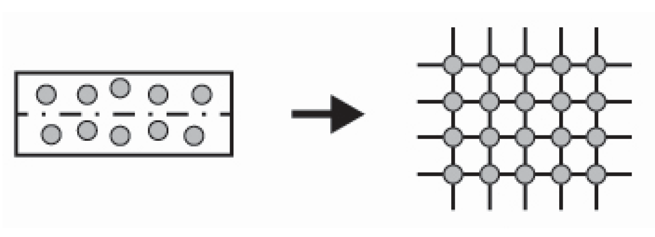
2.1. Microscale Level
2.2. Mesoscale Level
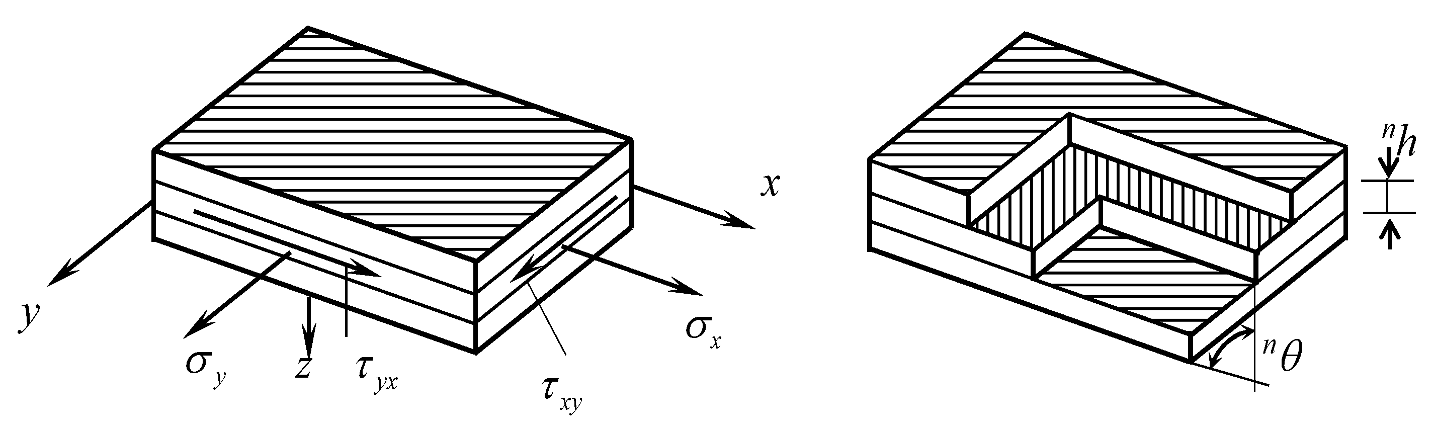
2.3. Macroscale Level
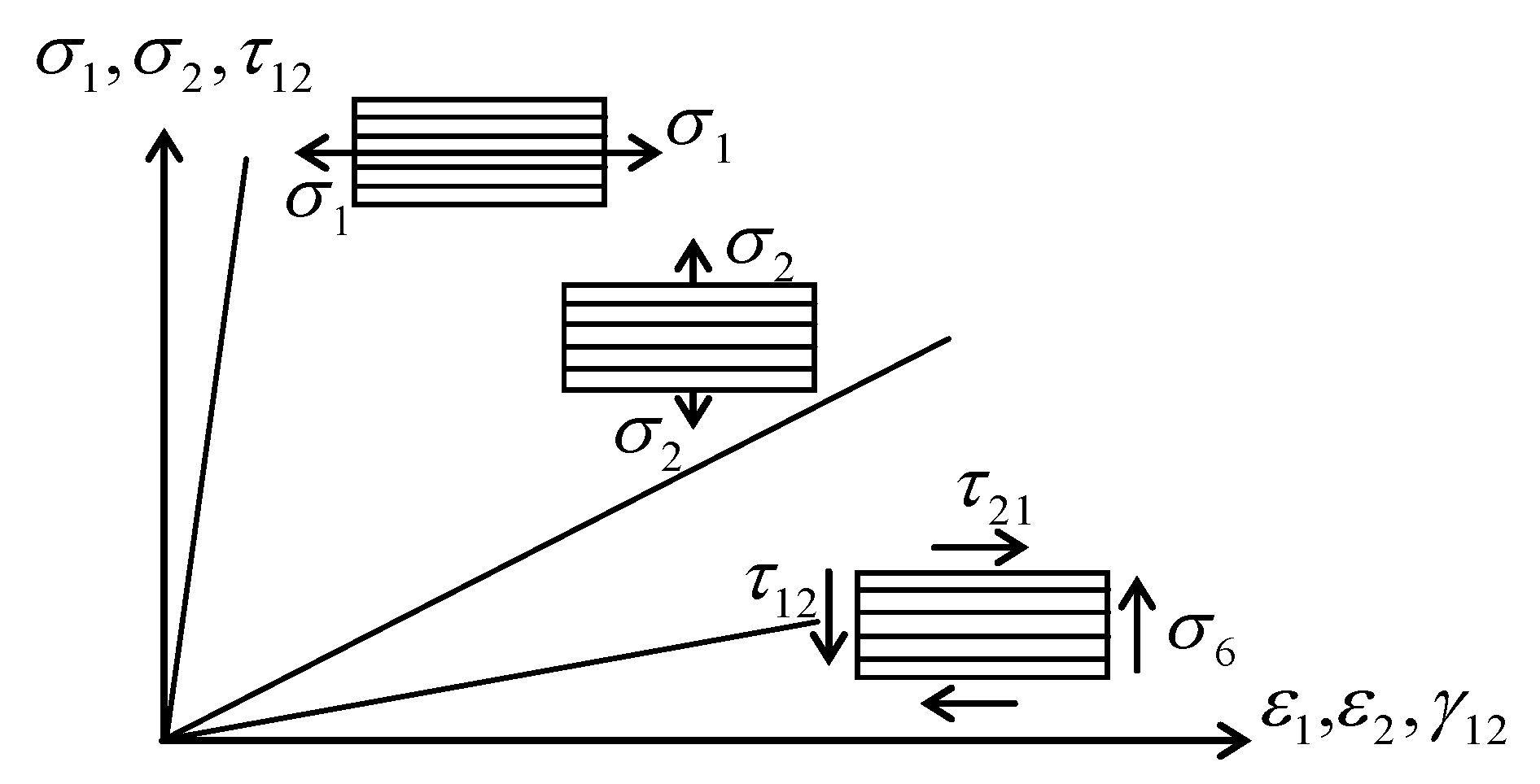
2.3.1. Classical Laminate Beam Theory
2.3.2. Shear Deformation Laminate Beam Theory
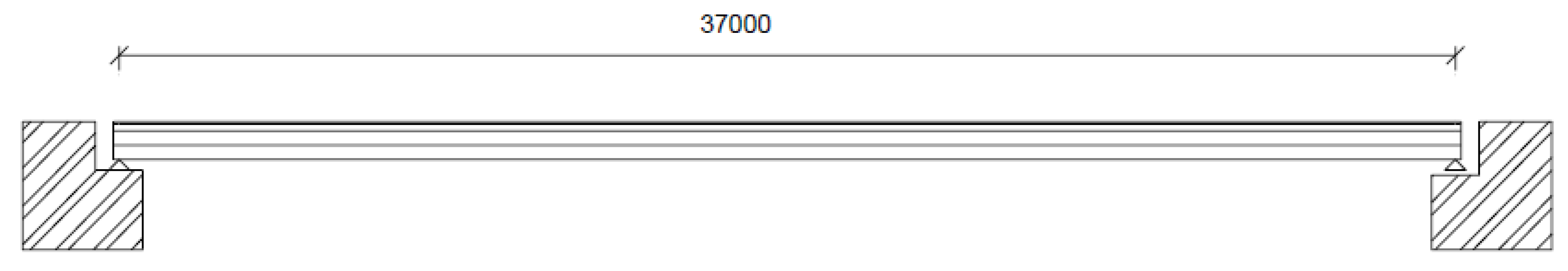
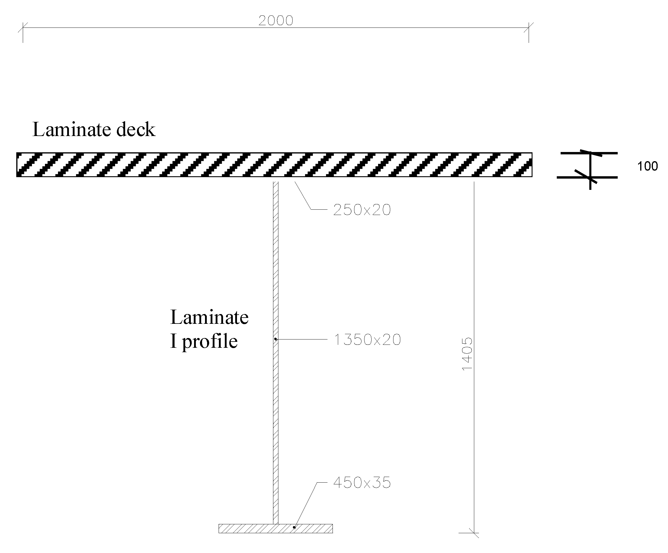
3. Bridge under Consideration, Discussion
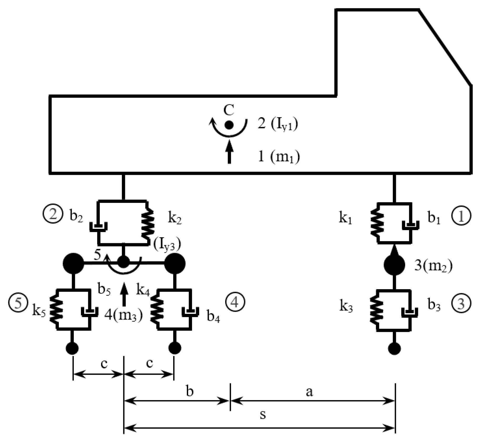
3.1. A Computational Model of Vehicle and Bridge
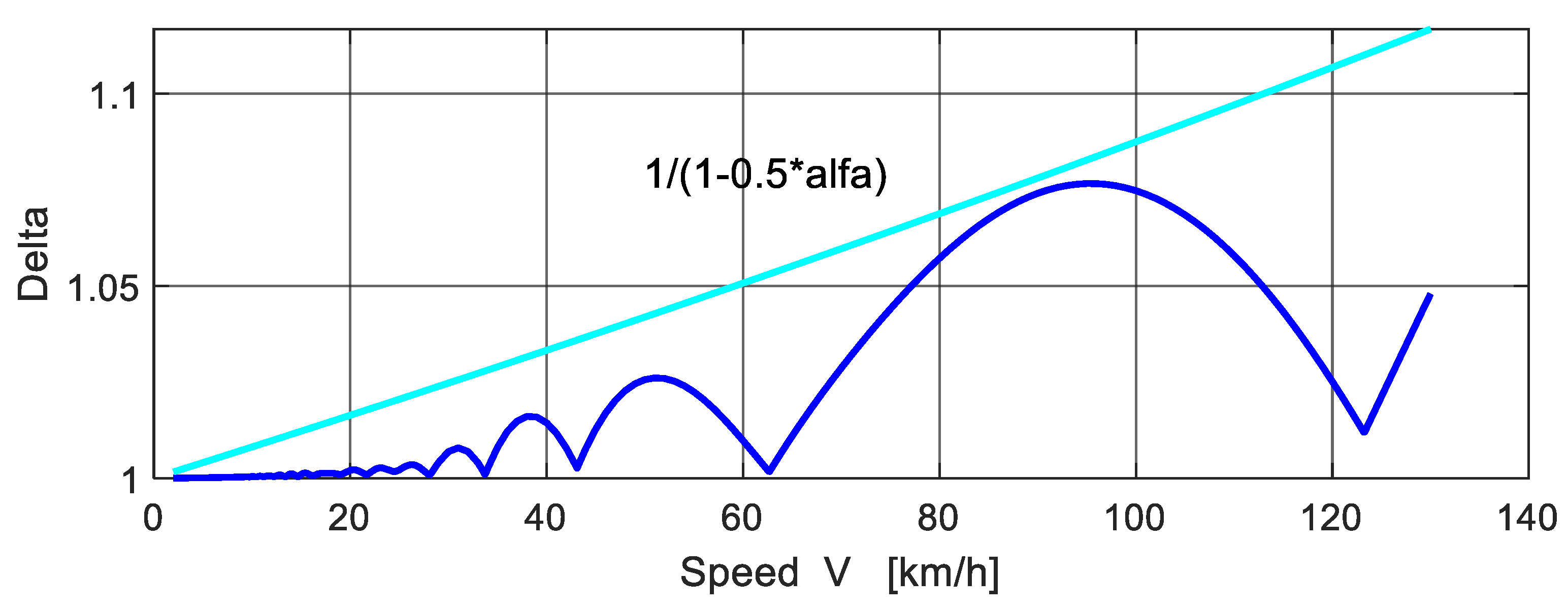
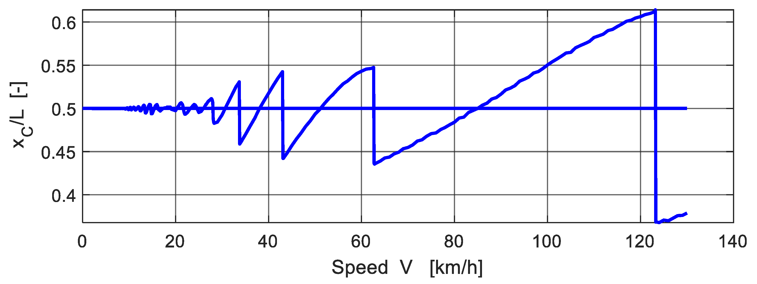
3.2. Results of Numerical Solution
4. Conclusions
Author Contributions
Funding
Institutional Review Board Statement
Informed Consent Statement
Data Availability Statement
Conflicts of Interest
References
- Agarwal, K.; Sahay, R.; Baji, A. Tensile Properties of Composite Reinforced with Three-Dimenssional Printed Fibers. Polymers 2020, 12, 1089. [Google Scholar] [CrossRef] [PubMed]
- Guessasma, S.; Belhabib, S.; Altin, A. On the Tensile Behaviour of Bio-Sourced 3D-Printed Structures from a Microstructural Perspective. Polymers 2020, 12, 1060. [Google Scholar] [CrossRef] [PubMed]
- Rajak, D.K.; Pagar, D.D.; Menezes P., L.; Linul, E. Fiber-Reinforced Polymer Composites: Manufacturing, Properties, and Applications. Polymers 2019, 11, 1667. [Google Scholar] [CrossRef] [PubMed] [Green Version]
- Simsek, M. Forced vibration of an embedded single-walled carbon nanotube traversed by a moving load using nonlocal Timoshenko beam theory. Steel Compos. Struct. 2011, 11, 59–76. [Google Scholar] [CrossRef]
- Shokrieh, M.M.; Shams Kondori, M. Effects of adding graphene nanoparticles in decreasing of residual stresses of carbon/epoxy laminated composites. Compos. Mater. Eng. 2020, 2, 53–64. [Google Scholar]
- Moon, J.; Ko, H.J.; Sung, I.H.; Lee, H.E. Natural frequency of a composite girder with corrugated steel web. Steel Compos. Struct. 2015, 18, 255–271. [Google Scholar] [CrossRef] [Green Version]
- Liu, X.; Li, F.; Wang, X. Synergistic effect of acidic environmental exposure and fatigue loads on FRP tendons. Constr. Build. Mat. 2022, 314, 125584. [Google Scholar] [CrossRef]
- Xian, G.; Guo, R.; Li, C. Combined effects of sustained bending loading, water immersion and fiber hybrid mode on the mechanical properties of carbon/glass fiber reinforced polymer composite. Comp. Struct. 2022, 281, 115060. [Google Scholar] [CrossRef]
- Rui, G.; Xian, G.J.; Li, F.; Li, C.; Hong, B. Hygrothermal resistance of pultruded carbon, glass and carbon/glass hybrid fiber reinforced epoxy composites. Constr. Build. Mater. 2022, 315, 125710. [Google Scholar]
- Melcer, J.; Lajčáková, G.; Martinická, I.; Králik, J. Dynamics of Transport Structures; EDIS: Žilina, Slovak, 2016. (In Slovak) [Google Scholar]
- Frýba, L. Vibration of Solids and Structures under Moving Loads; Prague Noordhoff International Publishing Groningen: Prague, Czech Republic, 1972. [Google Scholar]
- Fascetti, A.; Feo, L.; Abbaszadeh, H. A critical review of numerical methods for the simulation of pultruded fiber-reinforced structural elements. Compos. Struct. 2021, 273, 114284. [Google Scholar] [CrossRef]
- Kormanikova, E.; Zmindak, M.; Novak, P.; Sabol, P. Tensile properties of carbon fiber reinforced polymer matrix composites: Application for the strengthening of reinforced concrete structure. Compos. Struct. 2021, 275, 114448. [Google Scholar] [CrossRef]
- Cho, J.R. Natural element hierarchic models for the free vibration analyses of laminate composite plates. Compos. Struct. 2021, 272, 114147. [Google Scholar] [CrossRef]
- MATLAB 7.0.4 The Language of Technical Computing. Version 7, June 2005.
- Mirkhalaf, S.M.; Eggels, E.H.; Beurden, T.J.H.; Larsson, F.; Fagerstrom, M. A finite element based orientation averaging method for predicting elastic properties of short fiber reinforced composites. Compos. Part B Eng. 2020, 202, 108388. [Google Scholar] [CrossRef]
- Huang, Z.; Zhan, W.; Qian, X. Challenges for lightweight composites in the offshore and marine industry from the fatigue perspective. Compos. Mater. Eng. 2020, 2, 65–86. [Google Scholar]
- Shamsuddoha, M.; David, M.; Oromiehie, E.; Prusty, B.G. Distributed optical fibre sensor based monitoring of thermoplastic carbon composite cylinders under biaxial loading: Experimental and numerical investigations. Compos. Struct. 2021, 261, 113277. [Google Scholar] [CrossRef]
- Asyraf, M.R.M.; Ishak, M.R.; Sapuan, S.M.; Yidris, N. Utilization of Bracing Arms as Additional Reinforcement in Pultruded Glass Fiber-Reinforced Polymer Composite Cross-Arms: Creep Experimental and Numerical Analyses. Polymers 2021, 13, 620. [Google Scholar] [CrossRef]
- Krejčí, T.; Kruis, J.; Šejnoha, M.; Koudelka, T. Hybrid parallel approach to homogenization of transport processes in masonry. Adv. Eng. Softw. 2017, 113, 25–33. [Google Scholar] [CrossRef]
- Sahmani, S.; Safaei, B. Nonlocal strain gradient nonlinear resonance of bi-directional functionally graded composite micro/nano-beams under periodic soft excitation. Thin-Walled Struct. 2019, 143, 106226. [Google Scholar] [CrossRef]
- Lapcik, L.; Maňas, D.; Lapčíková, B.; Vašina, M.; Staněk, M.; Čépe, K.; Vlček, J.; Waters, K.E.; Greenwood, R.W.; Rowson, M.A. Effect of filler particle shape on plastic-elastic mechanical behavior of high density poly(ethylene)/mica and poly(ethylene)/wollastonite composites. Compos. Part B Eng. 2018, 14, 92–99. [Google Scholar] [CrossRef]
- Kormanikova, E.; Kotrasova, K. Micro-macro modelling of laminated composite rectangular reservoir. Compos. Struct. 2022, 279, 114701. [Google Scholar] [CrossRef]
- Safaei, B. Frequency-dependent damped vibrations of multifunctional foam plates sandwiched and integrated by composite faces. Eur. Phys. J. Plus 2021, 136, 646. [Google Scholar] [CrossRef]
- Mao, H.; Zhang, D.; Chen, L.; Zhao, Q.; Su, X.; Yuan, J. Flexural behaviour of a new lightweight glass fibre-reinforced polymer–metal string bridge with a box-truss composite girder. Adv. Struct. Eng. 2020, 23, 104–117. [Google Scholar] [CrossRef]
- Ali, H.T.; Yusuf, M.; Akrami, R.; Fotouhi, S.; Bodaghi, M.; Saeedifar, M.; Fotouhi, M. Fiber reinforced polymer composites in bridge industry. Structures 2021, 30, 774–785. [Google Scholar] [CrossRef]
- Potyrała, P.B. Use of Fibre Reinforced Polymers in Bridge Construction. State of the Art in Hybrid and All-Composite Structures. Master’s Thesis, Universitat Politecnica de Catalunya, Barcelona, Spain, 2011; pp. 1–93. [Google Scholar]
- Mahboob, A.; Gil, L.; Bernat-Maso, E.; Eskenati, A.R. Experimental and Numerical Study of Shear Interface Response of Hybrid Thin CFRP–Concrete Slabs. Materials 2021, 14, 5148. [Google Scholar] [CrossRef] [PubMed]
- Hu, W.; Li, Y.; Yuan, H. Review of Experimental Studies on Application of FRP for Strengthening of Bridge Structures. Adv. Mater. Sci. Eng. 2020, 2020, 8682163. [Google Scholar] [CrossRef]
- Melcer, J. Dynamic Calculations of Highway Bridges; EDIS, University of Žilina: Žilina-Vlčince, Slovakia, 1997. [Google Scholar]
- Melcer, J.; Sýkorová, R.; Václav, A. Dynamic coefficients of a bridge versus speed of vehicle motion. Civil Environ. Eng. 2009, 5, 96–109. [Google Scholar]
- Kotrasová, K.; Kormaníková, K. Dynamic analysis of liquid storage tanks. In Proceedings of the AIP Conference Proceedings: ICNAAM 2016, Thessaloniki, Greece, 25–30 September 2017; pp. 260005-1–260005-4. [Google Scholar]
- Kormanikova, E.; Kotrasova, K. Resonant frequencies and mode shapes of rectangular sandwich plate. Chemické Listy 2011, 105, 535–538. [Google Scholar]
- Vorel, J.; Sejnoha, M. Documentation for HELP Program, Theoretical Manual and User Guide; Czech Technical University in Prague: Prague, Czech Republic, 2008. [Google Scholar]
- Altenbach, H.; Altenbach, J.; Kissing, W. Mechanics of Composite Structural Elements; Springer: Berlin/Heidelberg, Germany, 2004. [Google Scholar]


| Property | Value |
|---|---|
| Mass density of the composite, ρ | 2100 kg/m3 |
| Longitudinal modulus, E1 | 214 GPa |
| Transverse modulus, E2 | 18.7 GPa |
| Longitudinal shear modulus, G12 | 4 GPa |
| Major in-plane Poisson’s ratio, ν12 | 0.27 |
| Fibre volume fraction, ξ | 0.55 |
| Effective moduli of laminate ((0/90)25)s, Ex = Eeff | 115 GPa |
| Effective shear modulus of laminate ((0/90)25)s, Geff | 4.8 GPa |
| Effective in-plane Poisson’s ratio of laminate, νeff | 0.035 |
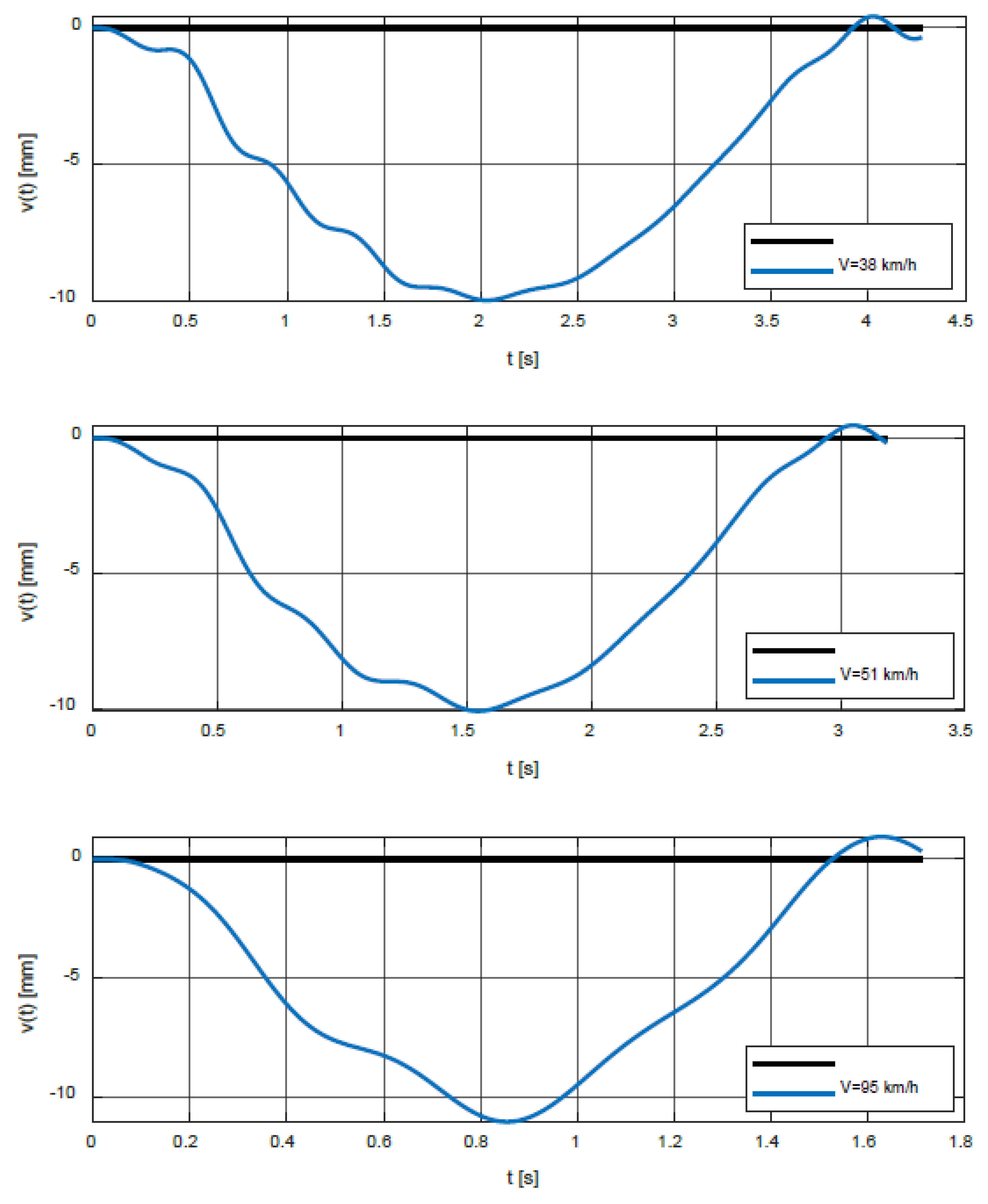
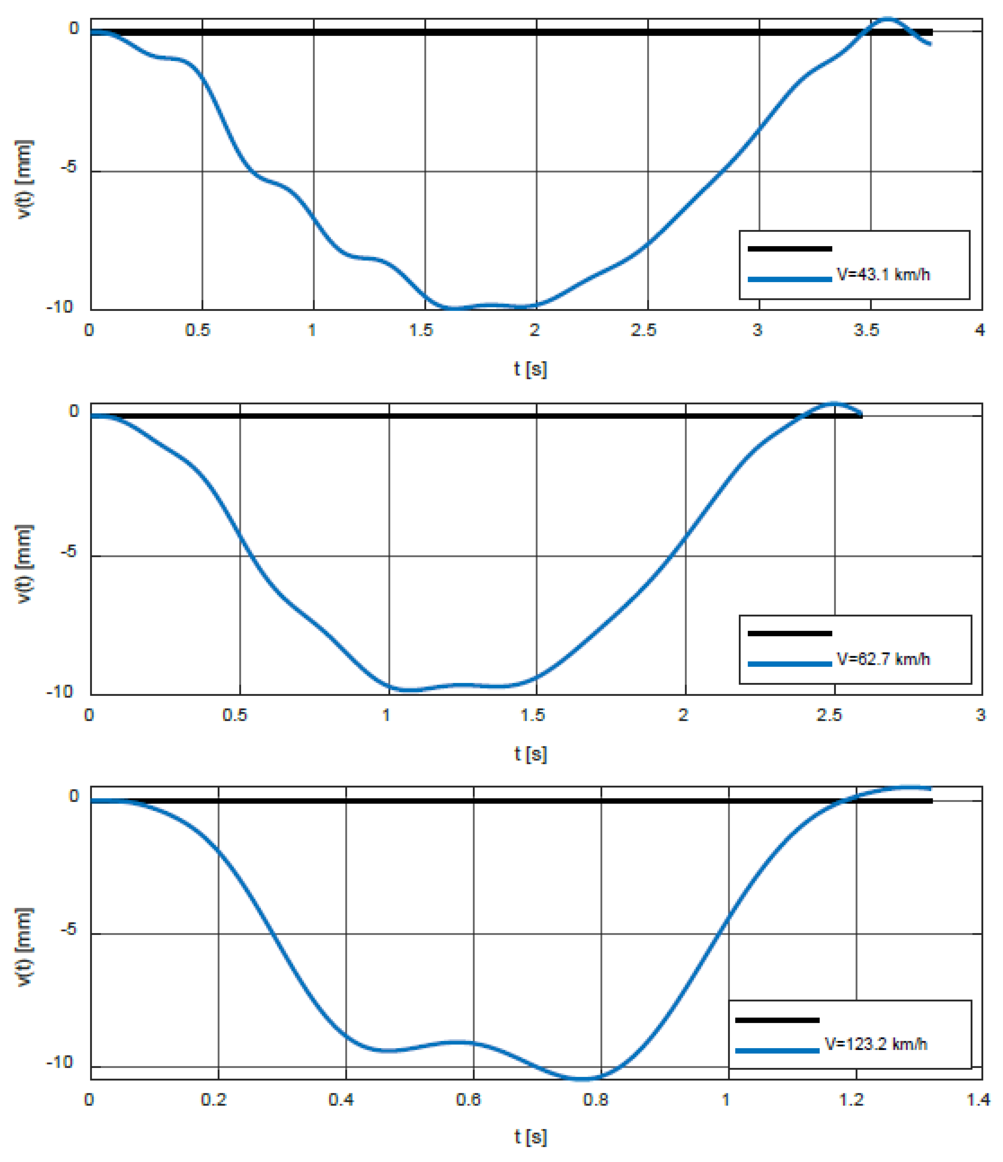
| Speed V (km/h) | tmax. (s) | Max. Dynamic Deflection vmax (mm) | Dynamic Factor δ |
|---|---|---|---|
| 38 | 2.0310 | 9.9627 | 1.0150 |
| 51 | 1.5432 | 10.1018 | 1.0292 |
| 95 | 0.8544 | 11.0073 | 1.1214 |
| 43.1 | 1.6296 | 9.9250 | 1.0112 |
| 62.7 | 1.0705 | 9.8174 | 1.0002 |
| 123.2 | 0.7711 | 10.4482 | 1.0645 |
Publisher’s Note: MDPI stays neutral with regard to jurisdictional claims in published maps and institutional affiliations. |
© 2022 by the authors. Licensee MDPI, Basel, Switzerland. This article is an open access article distributed under the terms and conditions of the Creative Commons Attribution (CC BY) license (https://creativecommons.org/licenses/by/4.0/).
Share and Cite
Kormanikova, E.; Kotrasova, K.; Melcer, J.; Valaskova, V. Numerical Investigation of the Dynamic Responses of Fibre-Reinforced Polymer Composite Bridge Beam Subjected to Moving Vehicle. Polymers 2022, 14, 812. https://doi.org/10.3390/polym14040812
Kormanikova E, Kotrasova K, Melcer J, Valaskova V. Numerical Investigation of the Dynamic Responses of Fibre-Reinforced Polymer Composite Bridge Beam Subjected to Moving Vehicle. Polymers. 2022; 14(4):812. https://doi.org/10.3390/polym14040812
Chicago/Turabian StyleKormanikova, Eva, Kamila Kotrasova, Jozef Melcer, and Veronika Valaskova. 2022. "Numerical Investigation of the Dynamic Responses of Fibre-Reinforced Polymer Composite Bridge Beam Subjected to Moving Vehicle" Polymers 14, no. 4: 812. https://doi.org/10.3390/polym14040812
APA StyleKormanikova, E., Kotrasova, K., Melcer, J., & Valaskova, V. (2022). Numerical Investigation of the Dynamic Responses of Fibre-Reinforced Polymer Composite Bridge Beam Subjected to Moving Vehicle. Polymers, 14(4), 812. https://doi.org/10.3390/polym14040812