
Characterization of Polyethylene Using a New Test Method Based on Stress Response to Relaxation and Recovery


Abstract
:1. Introduction
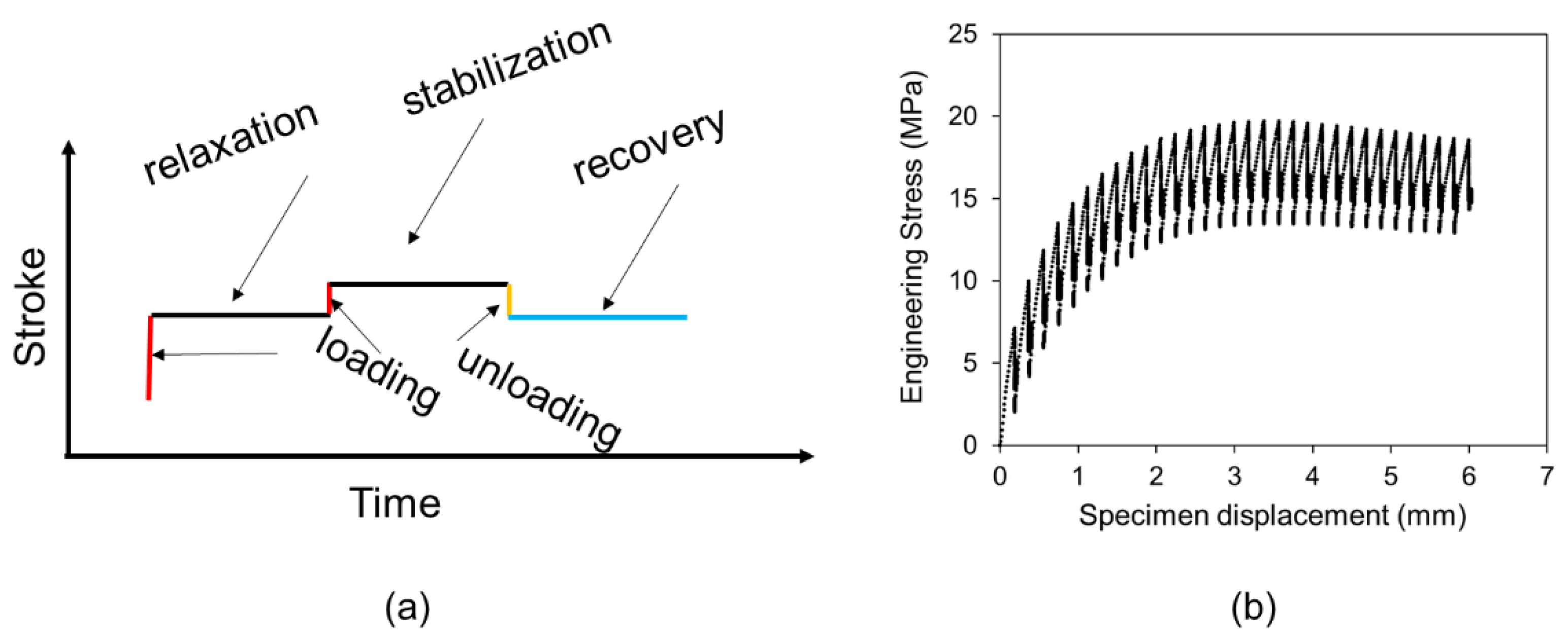
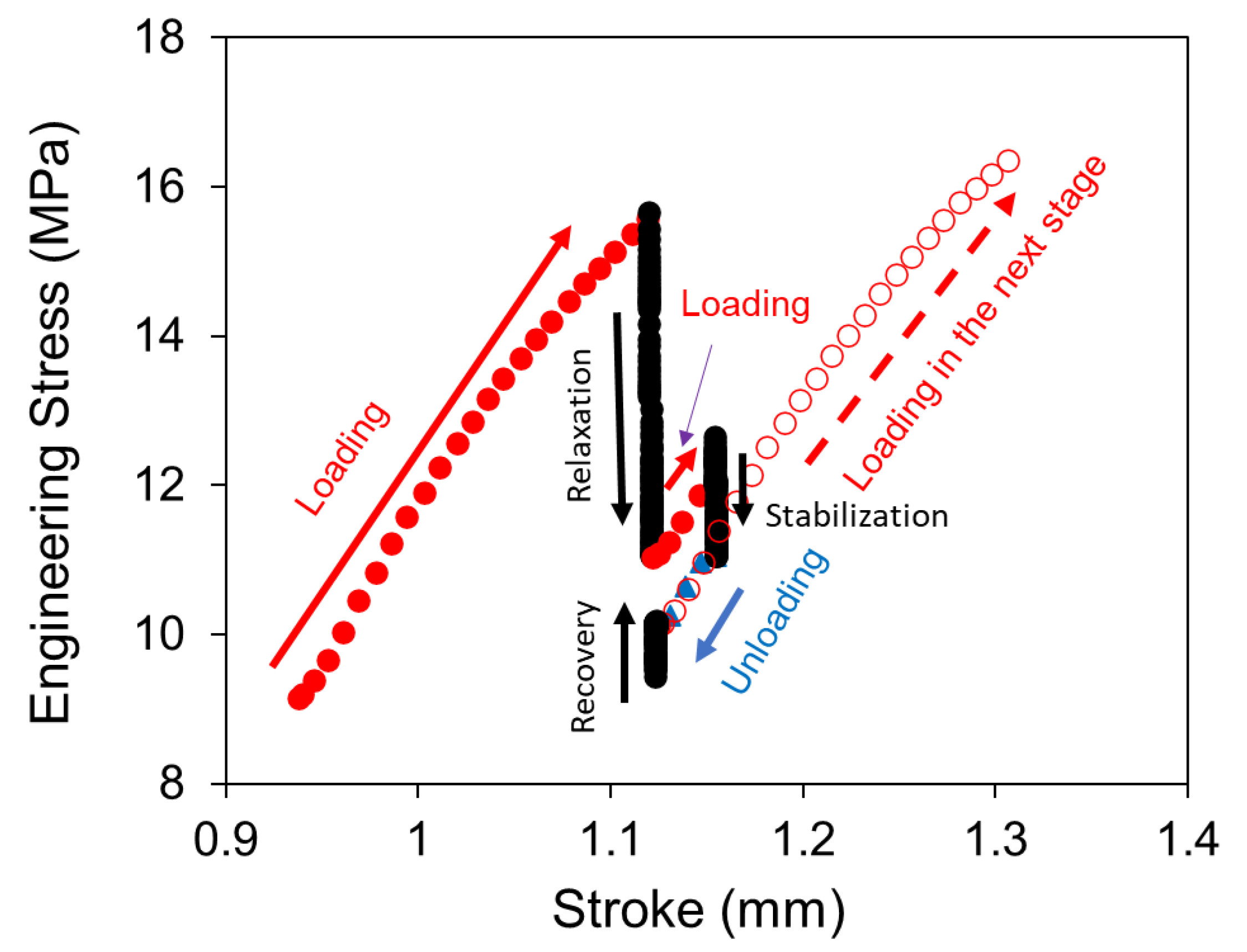
2. RR Test
3. Analysis of RR Test Results Based on Spring-Dashpot Models
3.1. Standard Model
3.2. Parallel Model
3.3. Series Model
4. Experimental Details of the RR Test Used in the Study
4.1. Materials and Specimen Dimensions
4.2. Test Conditions
5. Results and Discussion
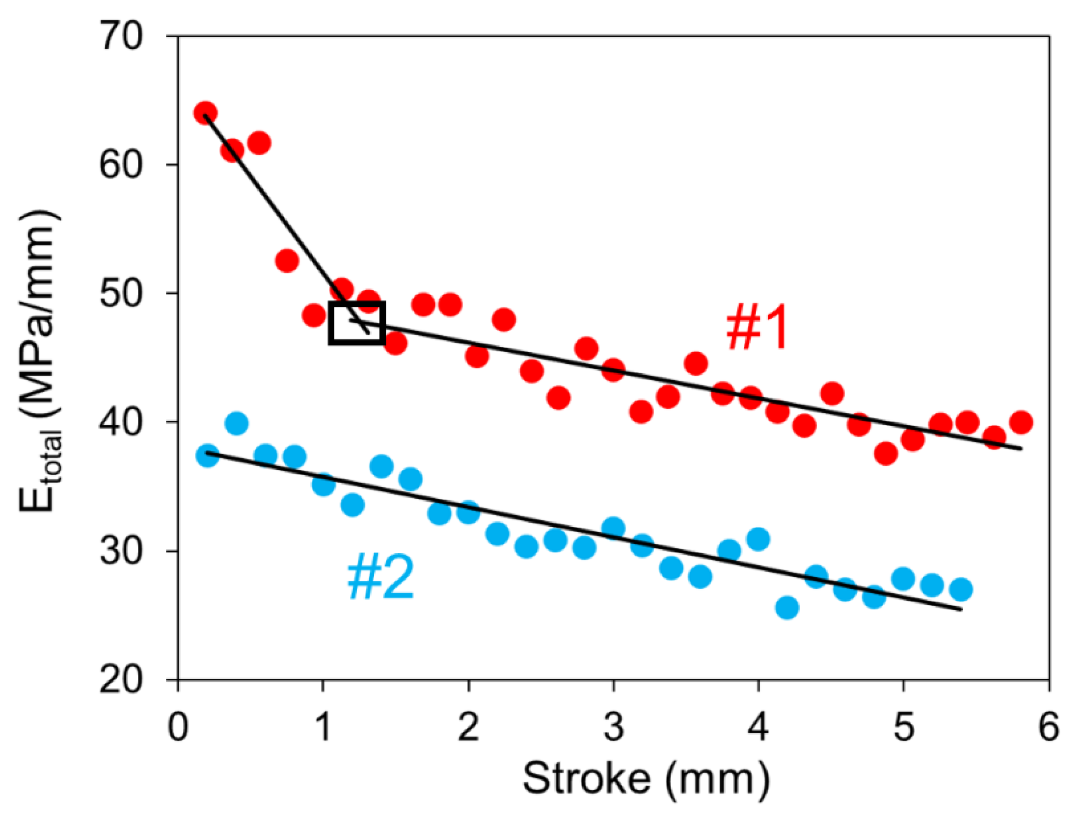
5.1. Case Study 1: Comparison of Three Models Depicted Above
5.2. Case Study 2: Determination of Activation Energies for the Eyring’s Model
6. Conclusions
Author Contributions
Funding
Data Availability Statement
Acknowledgments
Conflicts of Interest
References
- Geyer, R.; Jambeck, J.R.; Law, K.L. Production, Use, and Fate of All Plastics Ever Made. Sci. Adv. 2017, 3, e1700782. [Google Scholar] [CrossRef] [PubMed] [Green Version]
- Nguyen, K.Q.; Mwiseneza, C.; Mohamed, K.; Cousin, P.; Robert, M.; Benmokrane, B. Long-Term Testing Methods for HDPE Pipe-Advantages and Disadvantages: A Review. Eng. Fract. Mech. 2021, 246, 107629. [Google Scholar] [CrossRef]
- Qi, Z.; Hu, N.; Li, G.; Zeng, D.; Su, X. Constitutive Modeling for the Elastic-Viscoplastic Behavior of High Density Polyethylene under Cyclic Loading. Int. J. Plast. 2019, 113, 125–144. [Google Scholar] [CrossRef]
- Alsabri, A.; Al-Ghamdi, S.G. Carbon Footprint and Embodied Energy of PVC, PE, and PP Piping: Perspective on Environmental Performance. Energy Rep. 2020, 6, 364–370. [Google Scholar] [CrossRef]
- Ivanov, D.A. Semicrystalline Polymers. In Polymer Science: A Comprehensive Reference; Elsevier: Amsterdam, The Netherlands, 2012; pp. 227–258. ISBN 978-0-08-087862-1. [Google Scholar]
- Wu, K.; Zhang, H.; Liu, X.; Bolati, D.; Liu, G.; Chen, P.; Zhao, Y. Stress and Strain Analysis of Buried PE Pipelines Subjected to Mechanical Excavation. Eng. Fail. Anal. 2019, 106, 104171. [Google Scholar] [CrossRef]
- Krishnaswamy, P.; Shim, D.-J.; Kalyanam, S. Comparison of Parent and Butt-Fusion Material Properties of Unimodal High-Density Polyethylene. J. Press. Vessel Technol. 2017, 139, 041413. [Google Scholar] [CrossRef]
- Zha, S.; Lan, H.; Huang, H. Review on Lifetime Predictions of Polyethylene Pipes: Limitations and Trends. Int. J. Press. Vessel. Pip. 2022, 198, 104663. [Google Scholar] [CrossRef]
- Brown, N. Intrinsic Lifetime of Polyethylene Pipelines. Polym. Eng. Sci. 2007, 47, 477–480. [Google Scholar] [CrossRef] [Green Version]
- Zhang, Y.; Jar, P.-Y.B. Characterization of Ductile Damage in Polyethylene Based on Effective Stress Concept. Mech. Mater. 2019, 136, 103080. [Google Scholar] [CrossRef]
- Venkatesh, C. Performance Comparison of High Density Polyethylene Pipe (Hdpe) in Municipal Water Applications. Master’s Thesis, University of Texas at Arlington, Arlington, TX, USA, 2012. [Google Scholar]
- Majid, Z.A.; Mohsin, R.; Yaacob, Z.; Hassan, Z. Failure Analysis of Natural Gas Pipes. Eng. Fail. Anal. 2010, 17, 818–837. [Google Scholar] [CrossRef]
- Zhang, Y.; Chang, P.; Qiao, L.; Fan, J.; Xue, S.; Zhou, B. On the Estimation of Tensile Yield Stress for Polymer Materials Based on Punch Tests. Polym. Test. 2021, 100, 107249. [Google Scholar] [CrossRef]
- Zrida, M.; Laurent, H.; Rio, G.; Pimbert, S.; Grolleau, V.; Masmoudi, N.; Bradai, C. Experimental and Numerical Study of Polypropylene Behavior Using an Hyper-Visco-Hysteresis Constitutive Law. Comput. Mater. Sci. 2009, 45, 516–527. [Google Scholar] [CrossRef]
- Yeh, I.-C.; Andzelm, J.W.; Rutledge, G.C. Mechanical and Structural Characterization of Semicrystalline Polyethylene under Tensile Deformation by Molecular Dynamics Simulations. Macromolecules 2015, 48, 4228–4239. [Google Scholar] [CrossRef] [Green Version]
- Fritsch, J.; Hiermaier, S.; Strobl, G. Characterizing and Modeling the Non-Linear Viscoelastic Tensile Deformation of a Glass Fiber Reinforced Polypropylene. Compos. Sci. Technol. 2009, 69, 2460–2466. [Google Scholar] [CrossRef]
- Tan, N.; Jar, P.-Y.B. Determining Deformation Transition in Polyethylene under Tensile Loading. Polymers 2019, 11, 1415. [Google Scholar] [CrossRef] [Green Version]
- Izraylit, V.; Gould, O.E.C.; Rudolph, T.; Kratz, K.; Lendlein, A. Controlling Actuation Performance in Physically Cross-Linked Polylactone Blends Using Polylactide Stereocomplexation. Biomacromolecules 2020, 21, 338–348. [Google Scholar] [CrossRef]
- Alotta, G.; Barrera, O.; Pegg, E.C. Viscoelastic Material Models for More Accurate Polyethylene Wear Estimation. J. Strain Anal. Eng. Des. 2018, 53, 302–312. [Google Scholar] [CrossRef]
- Cangemi, L.; Meimon, Y. A Two-Phase Model for the Mechanical Behavior of Semicrystalline Polymers. Oil Gas Sci. Technol. Rev. IFP 2001, 56, 555–580. [Google Scholar] [CrossRef]
- Brusselle-Dupend, N.; Lai, D.; Feaugas, X.; Guigon, M.; Clavel, M. Mechanical Behavior of a Semicrystalline Polymer before Necking. Part II: Modeling of Uniaxial Behavior. Polym. Eng. Sci. 2003, 43, 501–518. [Google Scholar] [CrossRef]
- Drozdov, A.D.; de Claville Christiansen, J. Cyclic Viscoplasticity of High-Density Polyethylene: Experiments and Modeling. Comput. Mater. Sci. 2007, 39, 465–480. [Google Scholar] [CrossRef]
- Ames, N.M.; Srivastava, V.; Chester, S.A.; Anand, L. A Thermo-Mechanically Coupled Theory for Large Deformations of Amorphous Polymers. Part II: Applications. Int. J. Plast. 2009, 25, 1495–1539. [Google Scholar] [CrossRef] [Green Version]
- Boyce, M.C.; Socrate, S.; Llana, P.G. Constitutive Model for the Finite Deformation Stress–Strain Behavior of Poly(Ethylene Terephthalate) above the Glass Transition. Polymer 2000, 41, 2183–2201. [Google Scholar] [CrossRef]
- Mirkhalaf, S.M.; Andrade Pires, F.M.; Simoes, R. Modelling of the Post Yield Response of Amorphous Polymers under Different Stress States. Int. J. Plast. 2017, 88, 159–187. [Google Scholar] [CrossRef] [Green Version]
- Detrez, F.; Cantournet, S.; Séguéla, R. A Constitutive Model for Semi-Crystalline Polymer Deformation Involving Lamellar Fragmentation. Comptes Rendus Mécanique 2010, 338, 681–687. [Google Scholar] [CrossRef]
- Ward, I.M.; Sweeney, J. Mechanical Properties of Solid Polymers, 3rd ed.; Wiley: Chichester, UK, 2013; ISBN 978-1-4443-1950-7. [Google Scholar]
- O’Connor, T.C.; Robbins, M.O. Molecular Models for Creep in Oriented Polyethylene Fibers. J. Chem. Phys. 2020, 153, 144904. [Google Scholar] [CrossRef]
- Baled, H.O.; Gamwo, I.K.; Enick, R.M.; McHugh, M.A. Viscosity Models for Pure Hydrocarbons at Extreme Conditions: A Review and Comparative Study. Fuel 2018, 218, 89–111. [Google Scholar] [CrossRef]
- Yang, J.-L.; Zhang, Z.; Schlarb, A.K.; Friedrich, K. On the Characterization of Tensile Creep Resistance of Polyamide 66 Nanocomposites. Part II: Modeling and Prediction of Long-Term Performance. Polymer 2006, 47, 6745–6758. [Google Scholar] [CrossRef]
- Hong, K.; Rastogi, A.; Strobl, G. A Model Treating Tensile Deformation of Semicrystalline Polymers: Quasi-Static Stress−Strain Relationship and Viscous Stress Determined for a Sample of Polyethylene. Macromolecules 2004, 37, 10165–10173. [Google Scholar] [CrossRef]
- Izraylit, V.; Heuchel, M.; Gould, O.E.C.; Kratz, K.; Lendlein, A. Strain Recovery and Stress Relaxation Behaviour of Multiblock Copolymer Blends Physically Cross-Linked with PLA Stereocomplexation. Polymer 2020, 209, 122984. [Google Scholar] [CrossRef]
- Olley, P.; Sweeney, J. A Multiprocess Eyring Model for Large Strain Plastic Deformation. J. Appl. Polym. Sci. 2011, 119, 2246–2260. [Google Scholar] [CrossRef]
- Sweeney, J.; Bonner, M.; Ward, I.M. Modelling of Loading, Stress Relaxation and Stress Recovery in a Shape Memory Polymer. J. Mech. Behav. Biomed. Mater. 2014, 37, 12–23. [Google Scholar] [CrossRef] [Green Version]
- Chivers, R.A.; Bonner, M.J.; Hine, P.J.; Ward, I.M. Shape Memory and Stress Relaxation Behaviour of Oriented Mono-Dispersed Polystyrene. Polymer 2014, 55, 1055–1060. [Google Scholar] [CrossRef]
- Johnsen, J.; Clausen, A.H.; Grytten, F.; Benallal, A.; Hopperstad, O.S. A Thermo-Elasto-Viscoplastic Constitutive Model for Polymers. J. Mech. Phys. Solids 2019, 124, 681–701. [Google Scholar] [CrossRef]
- Xu, Q.; Solaimanian, M. Modelling Linear Viscoelastic Properties of Asphalt Concrete by the Huet–Sayegh Model. Int. J. Pavement Eng. 2009, 10, 401–422. [Google Scholar] [CrossRef]
- Halsey, G.; White, H.J.; Eyring, H. Mechanical Properties of Textiles, I. Text. Res. 1945, 15, 295–311. [Google Scholar] [CrossRef]
- Zhou, H.; Wilkes, G.L. Creep Behaviour of High Density Polyethylene Films Having Well-Defined Morphologies of Stacked Lamellae with and without an Observable Row-Nucleated Fibril Structure. Polymer 1998, 39, 3597–3609. [Google Scholar] [CrossRef]
- Siviour, C.R.; Jordan, J.L. High Strain Rate Mechanics of Polymers: A Review. J. Dyn. Behav. Mater. 2016, 2, 15–32. [Google Scholar] [CrossRef] [Green Version]
- Jar, P.-Y.B. Effect of Tensile Loading History on Mechanical Properties for Polyethylene. Polym. Eng. Sci. 2015, 55, 2002–2010. [Google Scholar] [CrossRef]
- Bao, Q.; Yang, Z.; Lu, Z. Molecular Dynamics Simulation of Amorphous Polyethylene (PE) under Cyclic Tensile-Compressive Loading below the Glass Transition Temperature. Polymer 2020, 186, 121968. [Google Scholar] [CrossRef]
- Gu, G.; Xia, Y.; Lin, C.; Lin, S.; Meng, Y.; Zhou, Q. Experimental Study on Characterizing Damage Behavior of Thermoplastics. Mater. Des. 2013, 44, 199–207. [Google Scholar] [CrossRef]
- Bergstrom, J. Constitutive Modeling of the Large Strain Time-Dependent Behavior of Elastomers. J. Mech. Phys. Solids 1998, 46, 931–954. [Google Scholar] [CrossRef]
- Shampine, L.F. Solving 0 = F(t, y(t), Y′(t)) in Matlab. J. Numer. Math. 2002, 291–310. [Google Scholar] [CrossRef]
- Senan, N.A.F. A Brief Introduction to Using Ode45 in MATLAB. University of California at Berkeley: Berkeley, CA, USA, 2007; Available online: https://www.eng.auburn.edu/~tplacek/courses/3600/ode45berkley.pdf (accessed on 3 July 2022).
- Tan, N.; Jar, P.B. Multi-Relaxation Test to Characterize PE Pipe Performance. Plast. Eng. 2019, 75, 40–45. [Google Scholar] [CrossRef]
- Kitagawa, M.; Zhou, D.; Qui, J. Stress-Strain Curves for Solid Polymers. Polym. Eng. Sci. 1995, 35, 1725–1732. [Google Scholar] [CrossRef]
- Richeton, J.; Ahzi, S.; Daridon, L.; Rémond, Y. A Formulation of the Cooperative Model for the Yield Stress of Amorphous Polymers for a Wide Range of Strain Rates and Temperatures. Polymer 2005, 46, 6035–6043. [Google Scholar] [CrossRef]
- Natarajan, V.D. Constitutive Behavior of a Twaron® Fabric/Natural Rubber Composite: Experiments and Modeling. Mech. Adv. Mater. Struct. 2011, 17, 246–259. [Google Scholar]
- Na, B.; Zhang, Q.; Fu, Q.; Men, Y.; Hong, K.; Strobl, G. Viscous-Force-Dominated Tensile Deformation Behavior of Oriented Polyethylene. Macromolecules 2006, 39, 2584–2591. [Google Scholar] [CrossRef]
- Senden, D.J.A.; van Dommelen, J.A.W.; Govaert, L.E. Physical Aging and Deformation Kinetics of Polycarbonate. J. Polym. Sci. B Polym. Phys. 2012, 50, 1589–1596. [Google Scholar] [CrossRef]
- Wilhelm, H.; Spieckermann, F.; Fischer, C.; Polt, G.; Zehetbauer, M. Characterization of Strain Bursts in High Density Polyethylene by Means of a Novel Nano Creep Test. Int. J. Plast. 2019, 116, 297–313. [Google Scholar] [CrossRef]
- Truss, R.W.; Duckett, R.A.; Ward, I.M. Effect of Hydrostatic Pressure on the Yield and Fracture of Polyethylene in Torsion. J. Mater. Sci 1981, 16, 1689–1699. [Google Scholar] [CrossRef]
- André, J.R.S.; Cruz Pinto, J.J.C. Modeling Nonlinear Stress Relaxation of Polymers. Polym. Eng. Sci. 2014, 54, 404–416. [Google Scholar] [CrossRef]


| Properties | Test Method | Units | HDPE-a | HDPE-b |
|---|---|---|---|---|
| Density | ASTM D792 | g/cm3 | 0.949 | 0.945 |
| Tensile Strength @ Yield | ASTM D638 | MPa | 24.1 | 22.5 |
| Ultimate Elongation | ASTM D638 | % | 500 | 850 |
| SCG PENT | ASTM F1473 | h | >10,000 | >100 |
Publisher’s Note: MDPI stays neutral with regard to jurisdictional claims in published maps and institutional affiliations. |
© 2022 by the authors. Licensee MDPI, Basel, Switzerland. This article is an open access article distributed under the terms and conditions of the Creative Commons Attribution (CC BY) license (https://creativecommons.org/licenses/by/4.0/).
Share and Cite
Shi, F.; Jar, P.-Y.B. Characterization of Polyethylene Using a New Test Method Based on Stress Response to Relaxation and Recovery. Polymers 2022, 14, 2763. https://doi.org/10.3390/polym14142763
Shi F, Jar P-YB. Characterization of Polyethylene Using a New Test Method Based on Stress Response to Relaxation and Recovery. Polymers. 2022; 14(14):2763. https://doi.org/10.3390/polym14142763
Chicago/Turabian StyleShi, Furui, and P.-Y. Ben Jar. 2022. "Characterization of Polyethylene Using a New Test Method Based on Stress Response to Relaxation and Recovery" Polymers 14, no. 14: 2763. https://doi.org/10.3390/polym14142763
APA StyleShi, F., & Jar, P.-Y. B. (2022). Characterization of Polyethylene Using a New Test Method Based on Stress Response to Relaxation and Recovery. Polymers, 14(14), 2763. https://doi.org/10.3390/polym14142763