
Modeling the Producibility of 3D Printing in Polylactic Acid Using Artificial Neural Networks and Fused Filament Fabrication


 , ,
, ,  ,
,
Abstract
:1. Introduction
2. Materials and Methods
2.1. Response Surface Methodology and Artificial Neural Network-Genetic Algorithm (ANN-GA)
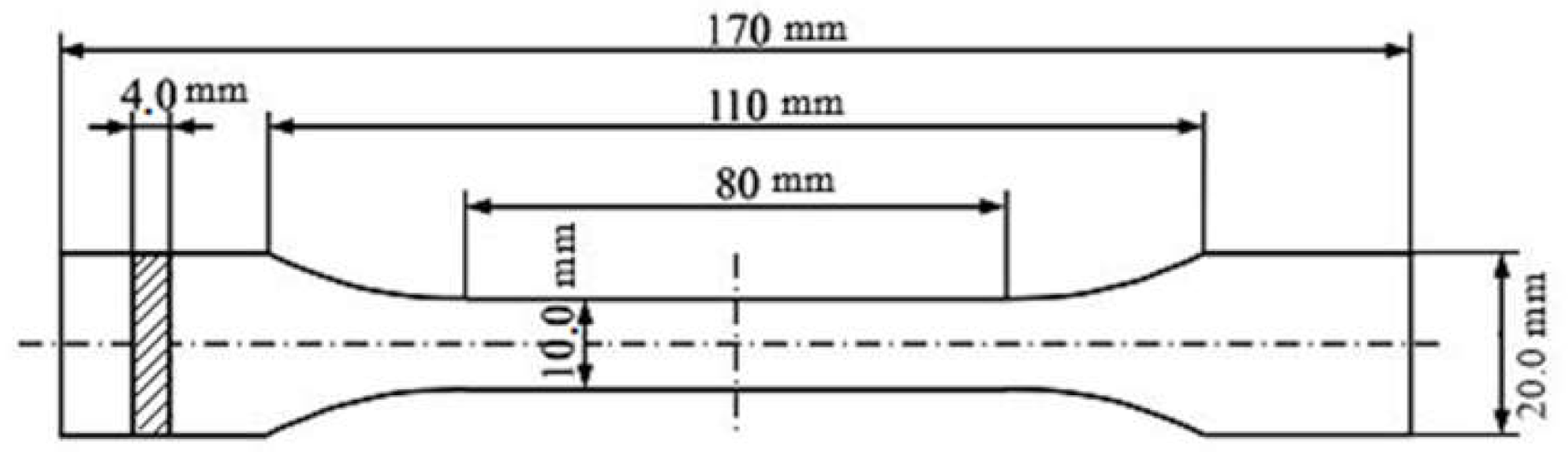
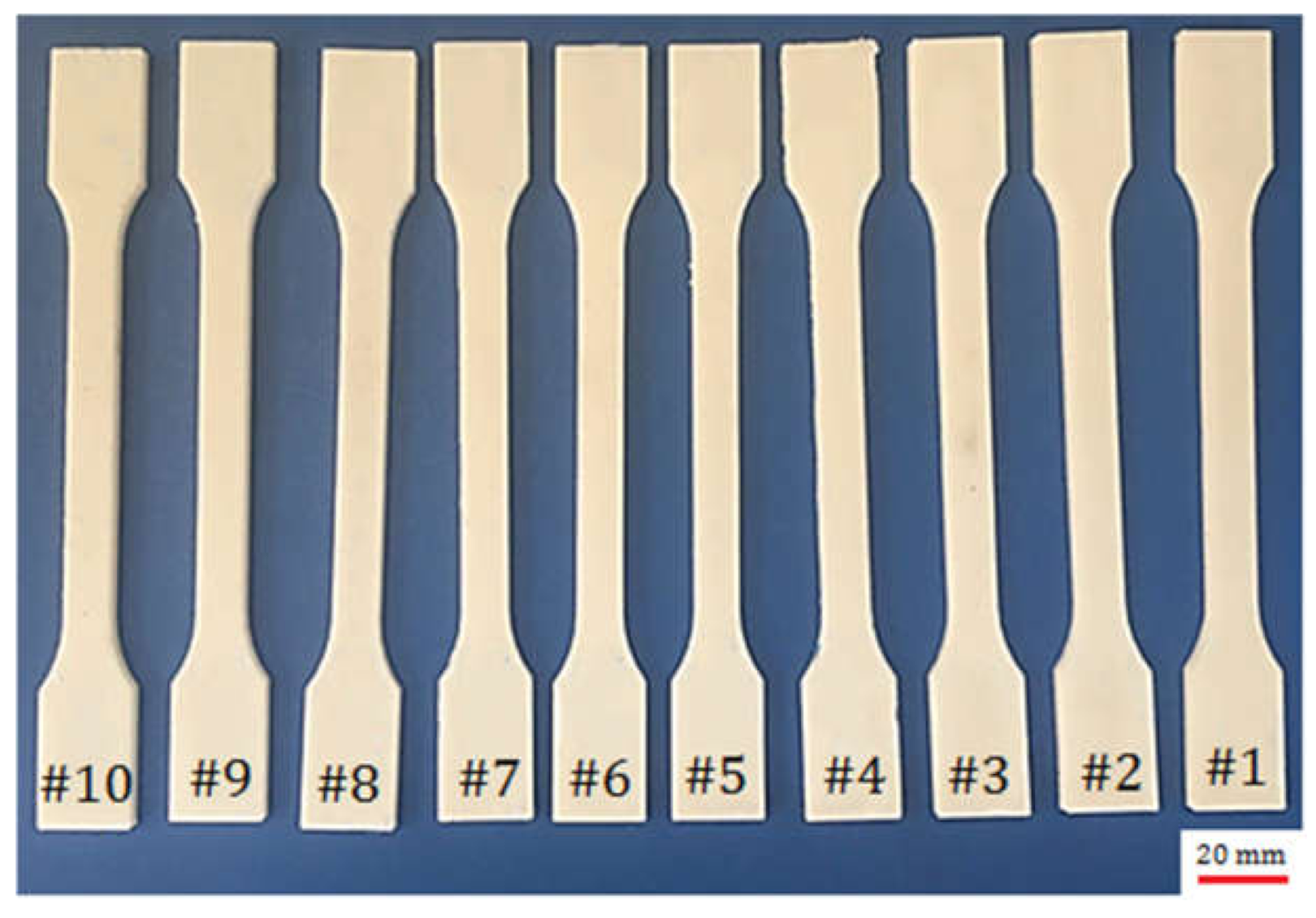
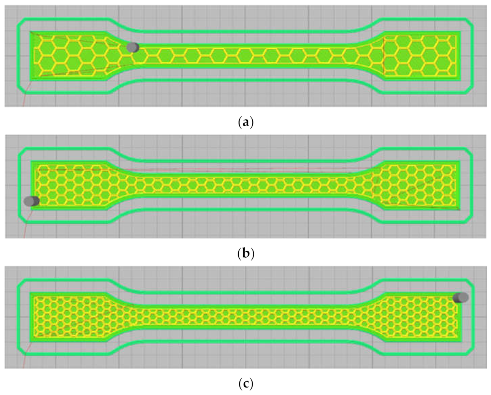
2.2. Experimental Work
3. Results
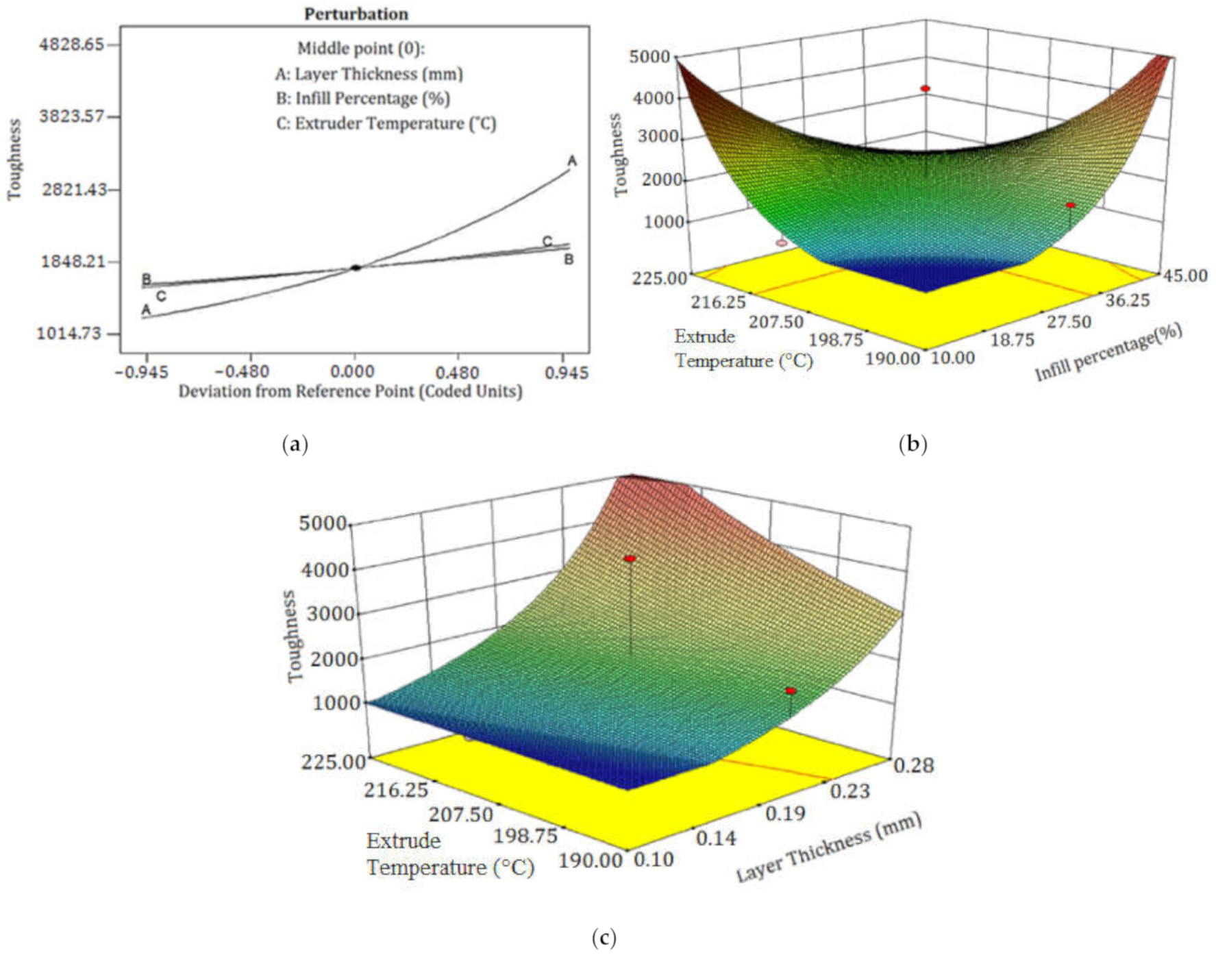
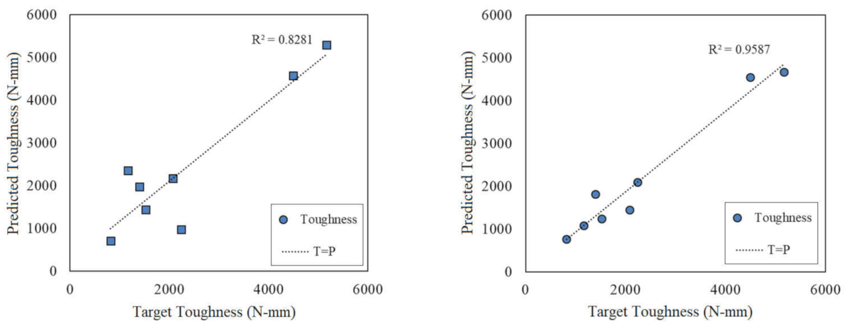
3.1. Toughness
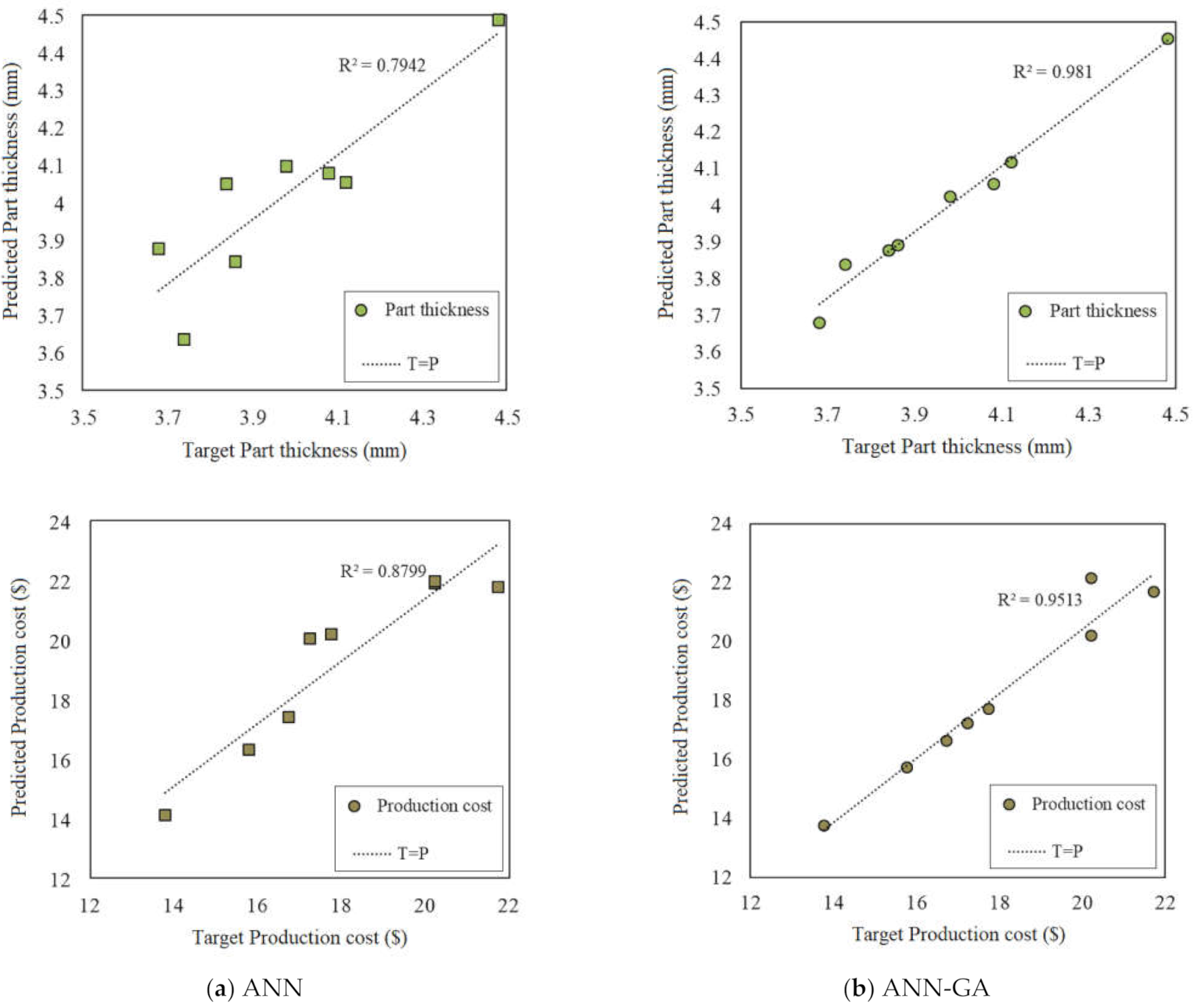
3.2. Part Thickness
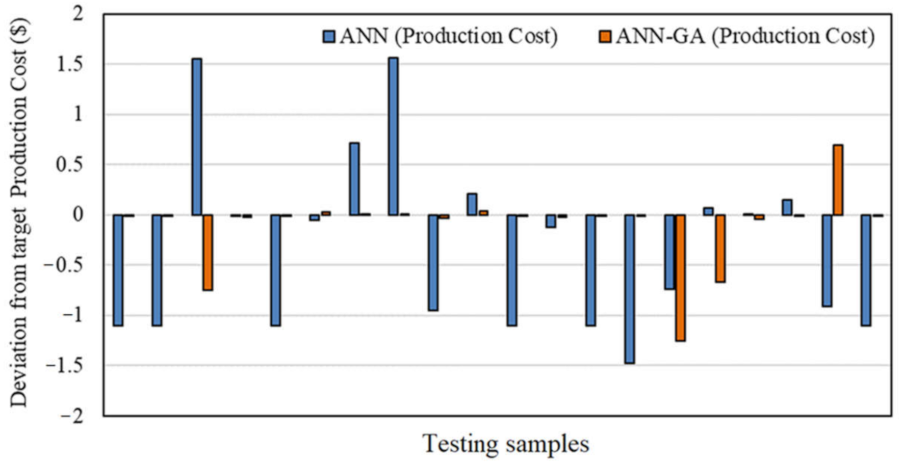
3.3. Production Cost
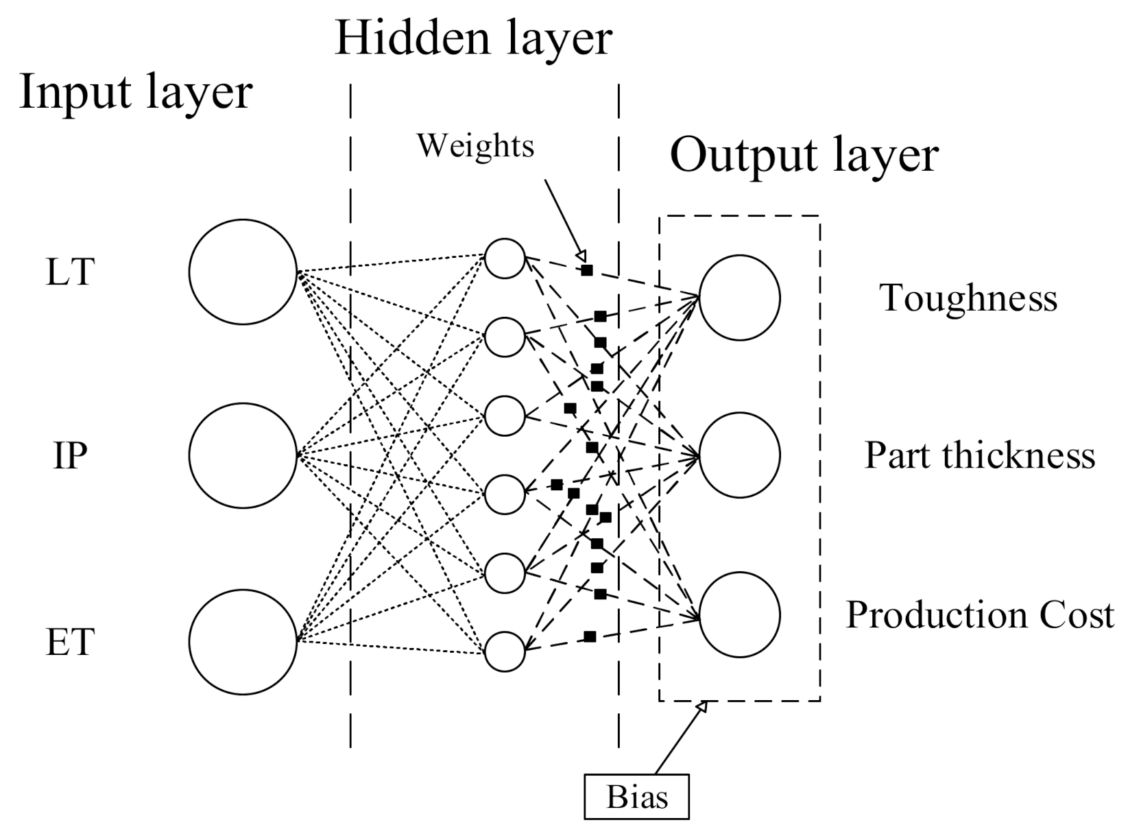
3.4. ANN and ANN-GA Techniques
3.5. Numerical Optimization
4. Conclusions
Author Contributions
Funding
Institutional Review Board Statement
Informed Consent Statement
Data Availability Statement
Acknowledgments
Conflicts of Interest
References
- Qattawi, A.; Alrawi, B.; Guzman, A. Experimental optimization of fused deposition modelling processing parameters: A design-for-manufacturing approach. Procedia Manuf. 2017, 10, 791–803. [Google Scholar]
- Sajan, N.; John, T.; Sivadasan, M.; Singh, N. An investigation on circularity error of components processed on Fused Deposition Modeling (FDM). Mater. Today 2018, 5, 1327–1334. [Google Scholar] [CrossRef]
- Sood, A.K.; Ohdar, R.; Mahapatra, S.S. Improving dimensional accuracy of fused deposition modelling processed part using grey Taguchi method. Mater. Des. 2009, 30, 4243–4252. [Google Scholar] [CrossRef]
- Liu, X.; Zhang, M.; Li, S.; Si, L.; Peng, J.; Hu, Y. Mechanical property parametric appraisal of fused deposition modeling parts based on the gray Taguchi method. Int. J. Adv. Manuf. Technol. 2017, 89, 2387–2397. [Google Scholar] [CrossRef]
- Dong, G.; Wijaya, G.; Tang, Y.; Zhao, Y.F. Optimizing process parameters of fused deposition modeling by Taguchi method for the fabrication of lattice structures. Addit. Manuf. 2018, 19, 62–72. [Google Scholar] [CrossRef] [Green Version]
- Mahmood, S.; Qureshi, A.; Talamona, D. Taguchi based process optimization for dimension and tolerance control for fused deposition modelling. Addit. Manuf. 2018, 21, 183–190. [Google Scholar] [CrossRef]
- Rao, R.V.; Rai, D.P. Optimization of fused deposition modeling process using teaching-learning-based optimization algorithm. Eng. Sci. Technol. Int. J. 2016, 19, 587–603. [Google Scholar] [CrossRef] [Green Version]
- Ceretti, E.; Ginestra, P.; Neto, P.; Fiorentino, A.; Da Silva, J. Multi-layered scaffolds production via Fused Deposition Modeling (FDM) using an open source 3D printer: Process parameters optimization for dimensional accuracy and design reproducibility. Procedia CIRP 2017, 65, 13–18. [Google Scholar] [CrossRef]
- Griffiths, C.; Howarth, J.; Rowbotham, G.D.-A.; Rees, A. Effect of build parameters on processing efficiency and material performance in fused deposition modelling. Procedia CIRP 2016, 49, 28–32. [Google Scholar] [CrossRef] [Green Version]
- Lieneke, T.; Denzer, V.; Adam, G.A.; Zimmer, D. Dimensional tolerances for additive manufacturing: Experimental investigation for Fused Deposition Modeling. Procedia CIRP 2016, 43, 286–291. [Google Scholar] [CrossRef] [Green Version]
- Rezaie, R.; Badrossamay, M.; Ghaie, A.; Moosavi, H. Topology optimization for fused deposition modeling process. Procedia CIRP 2013, 6, 521–526. [Google Scholar] [CrossRef] [Green Version]
- Ivanova, O.; Williams, C.; Campbell, T. Additive manufacturing (AM) and nanotechnology: Promises and challenges. Rapid Prototyp. J. 2013, 19, 353–364. [Google Scholar] [CrossRef] [Green Version]
- Buys, Y.; Aznan, A.; Anuar, H. Mechanical properties, morphology, and hydrolytic degradation behavior of polylactic acid/natural rubber blends. In Proceedings of the IOP Conference Series: Materials Science and Engineering (ICAMME 2017), Kuala Lumpur, Malaysia, 8–9 August 2017; IOP Publishing: Bristol, UK, 2018; p. 012077. [Google Scholar]
- Yadav, D.; Chhabra, D.; Gupta, R.K.; Phogat, A.; Ahlawat, A. Modeling and analysis of significant process parameters of FDM 3D printer using ANFIS. Mater. Today 2020, 21, 1592–1604. [Google Scholar] [CrossRef]
- Ali, F.; Chowdary, B.V. Natural Frequency prediction of FDM manufactured parts using ANN approach. IFAC Pap. 2019, 52, 403–408. [Google Scholar] [CrossRef]
- Sheoran, A.J.; Kumar, H. Fused Deposition modeling process parameters optimization and effect on mechanical properties and part quality: Review and reflection on present research. Mater. Today 2020, 21, 1659–1672. [Google Scholar]
- Moradi, M.; KaramiMoghadam, M. High power diode laser surface hardening of AISI 4130; statistical modelling and optimization. Opt. Laser Technol. 2019, 111, 554–570. [Google Scholar] [CrossRef]
- Moradi, M.; Karami Moghadam, M.; Shamsborhan, M.; Bodaghi, M.; Falavandi, H. Post-Processing of FDM 3D-Printed Polylactic Acid Parts by Laser Beam Cutting. Polymers 2020, 12, 550. [Google Scholar] [CrossRef] [PubMed] [Green Version]
- Azadi, M.; Azadi, S.; Zahedi, F.; Moradi, M. Multidisciplinary optimization of a car component under NVH and weight constraints using RSM. In Proceedings of the ASME 2009 International Mechanical Engineering Congress and Exposition, Lake Buena Vista, FL, USA, 13–19 November 2009; pp. 315–319. [Google Scholar]
- Plymill, A.; Minneci, R.; Greeley, D.A.; Gritton, J. Graphene and Carbon Nanotube PLA Composite Feedstock Development for Fused Deposition Modeling. Ph.D. Thesis, University of Tennessee, Knoxville, TN, USA, 2016. [Google Scholar]
- Benyounis, K.Y.; Olabi, A.G.; Hashmi, M.S.J. Mechanical properties, weld bead and cost universal approach for CO2 laser welding process optimisation. Int. J. Comput. Mater. Sci. Surf. Eng. 2009, 2, 99–109. [Google Scholar]
- Moradi, M.; Meiabadi, S.; Kaplan, A. 3D printed parts with honeycomb internal pattern by fused deposition modelling; experimental characterization and production optimization. Met. Mater. Int. 2019, 25, 1312–1325. [Google Scholar] [CrossRef]
- Sideratos, G.; Ikonomopoulos, A.; Hatziargyriou, N.D. A novel fuzzy-based ensemble model for load forecasting using hybrid deep neural networks. Electr. Power Syst. Res. 2020, 178, 106025. [Google Scholar] [CrossRef]
- Robinson, M.C.; Glen, R.C. Validating the validation: Reanalyzing a large-scale comparison of deep learning and machine learning models for bioactivity prediction. J. Comput. Aided Mol. Des. 2020, 20, 1–4. [Google Scholar] [CrossRef] [Green Version]
- Amid, S.; Gundoshmian, T.M. Prediction of output energies for broiler production using linear regression, ANN (MLP, RBF), and ANFIS models. Environ. Prog. Sustain. Energy 2017, 36, 577–585. [Google Scholar] [CrossRef]
- Chen, G.; Shen, Z.; Iyer, A.; Ghumman, U.F.; Tang, S.; Bi, J.; Chen, W.; Li, Y. Machine-Learning-Assisted De Novo Design of Organic Molecules and Polymers: Opportunities and Challenges. Polymers 2020, 12, 163. [Google Scholar] [CrossRef] [PubMed] [Green Version]
- Huang, L.; Ling, C. Practicing deep learning in materials science: An evaluation for predicting the formation energies. J. Appl. Phys. 2020, 128, 124901. [Google Scholar] [CrossRef]
- Mellit, A. ANN-based GA for generating the sizing curve of stand-alone photovoltaic systems. Adv. Eng. Softw. 2010, 41, 687–693. [Google Scholar] [CrossRef]
- Elbadawi, M.; Castro, B.M.; Gavins, F.K.; Ong, J.J.; Gaisford, S.; Pérez, G.; Basit, A.W.; Cabalar, P.; Goyanes, A. M3DISEEN: A novel machine learning approach for predicting the 3D printability of medicines. Int. J. Pharm. 2020, 590, 119837. [Google Scholar] [CrossRef]
- Hu, C.; Hau, W.N.J.; Chen, W.; Qin, Q.H. The fabrication of long carbon fiber reinforced polylactic acid composites via fused deposition modelling: Experimental analysis and machine learning. J. Compos. Mater. 2020, 55, 1459–1472. [Google Scholar] [CrossRef]
- Torres, J.; Cotelo, J.; Karl, J.; Gordon, A.P. Mechanical property optimization of FDM PLA in shear with multiple objectives. JOM 2015, 67, 1183–1193. [Google Scholar] [CrossRef]
- Moradi, M.; Karami Moghadam, M.; Shamsborhan, M.; Bodaghi, M. The synergic effects of FDM 3D printing parameters on mechanical behaviors of bronze poly lactic acid composites. J. Compos. Sci. 2020, 4, 17. [Google Scholar] [CrossRef] [Green Version]


| Factor | Unit | Levels | ||||
|---|---|---|---|---|---|---|
| −2 | −1 | 0 | 1 | 2 | ||
| LT | mm | 0.1 | 0.15 | 0.2 | 0.25 | 0.3 |
| IP | % | 10 | 20 | 30 | 40 | 50 |
| ET | C | 190 | 200 | 210 | 220 | 230 |
| Run | Input Factors | Output Responses | Type of Fracture | ||||
|---|---|---|---|---|---|---|---|
| LT | IP | ET | Toughness (N-mm) | Part Thickness (mm) | Production Cost ($) | ||
| 1 | 0.20 | 30.00 | 210.00 | 1829.27 | 3.98 | 17.73 | Brittle |
| 2 | 0.20 | 30.00 | 210.00 | 1394.35 | 3.84 | 17.73 | Brittle |
| 3 | 0.15 | 40.00 | 220.00 | 1157.86 | 3.88 | 21.72 | Brittle |
| 4 | 0.30 | 30.00 | 210.00 | 5164.36 | 3.68 | 13.77 | Tough |
| 5 | 0.20 | 30.00 | 210.00 | 1674.03 | 4.02 | 17.73 | Brittle |
| 6 | 0.25 | 40.00 | 200.00 | 5144.17 | 4.00 | 15.76 | Tough |
| 7 | 0.25 | 20.00 | 200.00 | 1835.62 | 3.82 | 15.25 | Brittle |
| 8 | 0.15 | 20.00 | 220.00 | 2239.94 | 4.48 | 20.2 | Brittle |
| 9 | 0.20 | 30.00 | 210.00 | 4112.96 | 4.04 | 17.73 | Tough |
| 10 | 0.15 | 40.00 | 200.00 | 1520.79 | 3.98 | 21.72 | Brittle |
| 11 | 0.20 | 30.00 | 210.00 | 1140.16 | 4.08 | 17.73 | Brittle |
| 12 | 0.20 | 10.00 | 210.00 | 1167.21 | 3.86 | 16.72 | Brittle |
| 13 | 0.10 | 30.00 | 210.00 | 830.976 | 3.98 | 27.19 | Brittle |
| 14 | 0.15 | 20.00 | 200.00 | 817.052 | 4.08 | 20.2 | Brittle |
| 15 | 0.20 | 30.00 | 230.00 | 2644.34 | 4.08 | 17.23 | Brittle |
| 16 | 0.20 | 30.00 | 190.00 | 2075.45 | 3.74 | 17.23 | Brittle |
| 17 | 0.20 | 50.00 | 210.00 | 2462.57 | 3.9 | 18.25 | Brittle |
| 18 | 0.25 | 40.00 | 220.00 | 4489.05 | 4.12 | 15.76 | Tough |
| 19 | 0.25 | 20.00 | 220.00 | 5046.5 | 3.8 | 15.25 | Tough |
| 20 | 0.20 | 30.00 | 210.00 | 1393.06 | 3.86 | 17.73 | Brittle |
| Accuracy and Performance Index | Description |
|---|---|
| Correlation coefficient = |
|
| RMSE = |
| Property | Value |
|---|---|
| Full name | Polylactic acid (PLA) |
| Melting point | 150 to 160 °C (302 to 320 °F) |
| Glass transition | 60–65 °C |
| Injection mold temperature | 178 to 240 °C (353 to 464 °F) |
| Density | 1.210–1.430 g·cm−3 |
| Chemical formula | (C3H4O2)n |
| Crystallinity | 37% |
| Tensile modulus | 2.7–16 GPa |
| molecular weight (Mw) | 112 kg/mol ± 1733 |
| Polydispersity (MW/MN) | 1.65 ± 0.05 |
| No | Build Parameters | Unit | Value |
|---|---|---|---|
| 1 | Nozzle diameter | mm | 0.45 |
| 2 | Extrusion width | mm | 0.45 |
| 3 | Top solid layer | - | 6 |
| 4 | Bottom solid layers | - | 6 |
| 5 | Default printing speed | mm/min | 3600 |
| 6 | Retraction speed | mm/min | 1800 |
| 7 | Outline overlap | - | Full honeycomb |
| 8 | Interior fill percentage | % | 15 |
| Source | Sum of Squares (SOS) | Df | Mean Square (MS) | F-Value (F-v) | P-Value (P-v) |
|---|---|---|---|---|---|
| Model | 1.694 × 10⁻³ | 4 | 4.235 × 10⁻⁴ | 13.04 | <0.0001 |
| LT | 1.228 × 10⁻³ | 1 | 1.228 × 10⁻³ | 37.81 | <0.0001 |
| IP | 1.250 × 10⁻⁴ | 1 | 1.250 × 10⁻⁴ | 3.85 | 0.0687 |
| ET | 8.980 × 10⁻⁵ | 1 | 8.980 × 10⁻⁵ | 2.76 | 0.1171 |
| (IP) × (ET) | 2.513 × 10⁻⁴ | 1 | 2.513 × 10⁻⁴ | 7.74 | 0.0140 |
| Residual | 4.872 × 10⁻⁴ | 15 | 3.248 × 10⁻⁵ | ||
| Lack of Fit (LOF) | 1.747 × 10⁻⁴ | 10 | 1.747 × 10⁻⁵ | 0.28 | 0.9591 |
| Pure Error (PR) | 3.125 × 10⁻⁴ | 5 | 6.250 × 10⁻⁵ | ||
| Cor Total (CT) | 2.181 × 10⁻³ | 19 | |||
| Pred R-Square | 0.6747 | Adj R-Squared | 0.7171 | R-Squared | 0.7766 |
| Source | SOS | Df | MS | F-v | P-v |
|---|---|---|---|---|---|
| Model | 0.89 | 6 | 0.15 | 4.46 | 0.0115 |
| LT | 0.20 | 1 | 0.20 | 5.98 | 0.0294 |
| IP | 0.024 | 1 | 0.024 | 0.73 | 0.4096 |
| E) | 0.15 | 1 | 0.15 | 4.48 | 0.0542 |
| (LT) × (IP) | 0.36 | 1 | 0.36 | 10.92 | 0.0057 |
| (LT) × (ET) | 0.061 | 1 | 0.061 | 1.85 | 0.1968 |
| (IP) × (ET) | 0.092 | 1 | 0.092 | 2.79 | 0.1185 |
| Residual | 0.43 | 13 | 0.033 | ||
| PR | 0.049 | 5 | 9720 × 10−3 | ||
| LOF | 0.38 | 8 | 0.048 | 4.91 | 0.0482 |
| CT | 1.32 | 19 | |||
| Pred R-Square | −0.5694 | Adj R-Squared | 0.5220 | R-Squared | 0.6730 |
| Source | SOS | Df | MS | F-v | P-v |
|---|---|---|---|---|---|
| Model | 6.769 × 10⁻⁵ | 5 | 1.354 × 10⁻⁵ | 1464.91 | <0.0001 |
| LT | 6.592 × 10⁻⁵ | 1 | 6.592 × 10⁻⁵ | 7133.12 | <0.0001 |
| IP | 1.555 × 10⁻⁶ | 1 | 1.555 × 10⁻⁶ | 168.23 | <0.0001 |
| ET | 0.000 | 1 | 0.000 | 0.000 | 1.0000 |
| IP2 | 4.940 × 10⁻⁸ | 1 | 4.940 × 10⁻⁸ | 5.35 | 0.0365 |
| ET2 | 1.927 × 10⁻⁷ | 1 | 1.927 × 10⁻⁷ | 20.85 | 0.0004 |
| PE | 0.000 | 5 | 0.000 | ||
| LOF | 1.294 × 10⁻⁷ | 9 | 1.438 × 10⁻⁸ | ||
| Residual | 1.294 × 10⁻⁷ | 14 | 9.241 × 10⁻⁹ | ||
| CT | 6.782 × 10⁻⁵ | 19 | |||
| Pred R-Square | 0.9940 | Adj R-Squared | 0.9974 | R-Squared | 0.9981 |
| Output Factor | ANN | Correlation Coefficient | RMSE | ANN-GA | Correlation Coefficient | RMSE | |
|---|---|---|---|---|---|---|---|
| No. of Neurons | Pop. Size | Max Gen. | |||||
| Toughness (N-mm) | 10 | 0.7877 | 924.5529274 | 50 | 320 | 0.9439 | 633.6373621 |
| 12 | 0.8782 | 908.0737946 | 100 | 210 | 0.8692 | 734.6853877 | |
| 14 | 0.7964 | 893.2048644 | 150 | 360 | 0.9642 | 453.8843405 | |
| 16 | 0.8789 | 694.1594251 | 200 | 110 | 0.9186 | 654.6824998 | |
| Part thickness (mm) | 10 | 0.7671 | 0.12949 | 50 | 320 | 0.9362 | 0.045035408 |
| 12 | 0.8788 | 0.075333178 | 100 | 210 | 0.93 | 0.042059003 | |
| 14 | 0.5173 | 0.084915266 | 150 | 360 | 0.7768 | 0.059754932 | |
| 16 | 0.6324 | 0.099691882 | 200 | 110 | 0.8538 | 0.077821436 | |
| Production cost ($) | 10 | 0.8531 | 1.960663 | 50 | 320 | 09485 | 1.288136157 |
| 12 | 0.9636 | 0.970732923 | 100 | 210 | 0.8956 | 1.556494043 | |
| 14 | 0.8235 | 3.830106928 | 150 | 360 | 0.9754 | 1.011613758 | |
| 16 | 0.842 | 2.267871729 | 200 | 110 | 0.9105 | 1.29979527 | |
| Output Factor | ANN | Correlation Coefficient | RMSE | ANN-GA | Correlation Coefficient | RMSE | |
|---|---|---|---|---|---|---|---|
| No. of Neurons | Pop. Size | Max Gen. | |||||
| Toughness (N-mm) | 12 | 0.91 | 651.7539629 | 150 | 360 | 0.9791 | 277.4633823 |
| Part thickness (mm) | 0.8911 | 0.118439425 | 0.9904 | 0.036062371 | |||
| Production Cost ($) | 0.938 | 0.861473905 | 0.9762 | 0.569953845 | |||
| Responses/Parameters | Name | Goal | Lower Limit | Upper Limit | Lower Weight | Upper Weight | Importance | |
|---|---|---|---|---|---|---|---|---|
| Parameters | LT | Is in range | 0.1 | 0.3 | 1 | 1 | - | |
| IP | Is in range | 10 | 50 | 1 | 1 | - | ||
| ET | Is in range | 190 | 230 | 1 | 1 | - | ||
| Responses | Criteria | Toughness | Maximum | 817 | 5500 | 1 | 1 | 1 |
| Thickness | is goal = 4 | 3.68 | 4.98 | 1 | 1 | 1 | ||
| Cost | Minimum | 13.77 | 27.19 | 1 | 1 | 1 | ||
| Sol. | Optimum Inputs | Desirability | Output Responses | |||||
|---|---|---|---|---|---|---|---|---|
| LT | IP | ET | Toughness (N-mm) | Thickness (mm) | Production Cost ($) | |||
| 1 | 0.28 | 38 | 222 | 0.99 | Actual | 5097.727 | 3.72 | 14.77 |
| Predicted | 5399.99 | 4.000 | 14.372 | |||||
| Error% | −5.93% | −7.5% | 2.23% | |||||
Publisher’s Note: MDPI stays neutral with regard to jurisdictional claims in published maps and institutional affiliations. |
© 2021 by the authors. Licensee MDPI, Basel, Switzerland. This article is an open access article distributed under the terms and conditions of the Creative Commons Attribution (CC BY) license (https://creativecommons.org/licenses/by/4.0/).
Share and Cite
Meiabadi, M.S.; Moradi, M.; Karamimoghadam, M.; Ardabili, S.; Bodaghi, M.; Shokri, M.; Mosavi, A.H. Modeling the Producibility of 3D Printing in Polylactic Acid Using Artificial Neural Networks and Fused Filament Fabrication. Polymers 2021, 13, 3219. https://doi.org/10.3390/polym13193219
Meiabadi MS, Moradi M, Karamimoghadam M, Ardabili S, Bodaghi M, Shokri M, Mosavi AH. Modeling the Producibility of 3D Printing in Polylactic Acid Using Artificial Neural Networks and Fused Filament Fabrication. Polymers. 2021; 13(19):3219. https://doi.org/10.3390/polym13193219
Chicago/Turabian StyleMeiabadi, Mohammad Saleh, Mahmoud Moradi, Mojtaba Karamimoghadam, Sina Ardabili, Mahdi Bodaghi, Manouchehr Shokri, and Amir H. Mosavi. 2021. "Modeling the Producibility of 3D Printing in Polylactic Acid Using Artificial Neural Networks and Fused Filament Fabrication" Polymers 13, no. 19: 3219. https://doi.org/10.3390/polym13193219
APA StyleMeiabadi, M. S., Moradi, M., Karamimoghadam, M., Ardabili, S., Bodaghi, M., Shokri, M., & Mosavi, A. H. (2021). Modeling the Producibility of 3D Printing in Polylactic Acid Using Artificial Neural Networks and Fused Filament Fabrication. Polymers, 13(19), 3219. https://doi.org/10.3390/polym13193219