
Simulation Approach for Hydrophobicity Replication via Injection Molding


Abstract
:
1. Introduction
2. Materials and Methods
2.1. Mathematical Formulation
2.2. Mold Properties for Plastic Injection
2.3. Polymer Properties for Plastic Injections
2.4. Simulation Setup
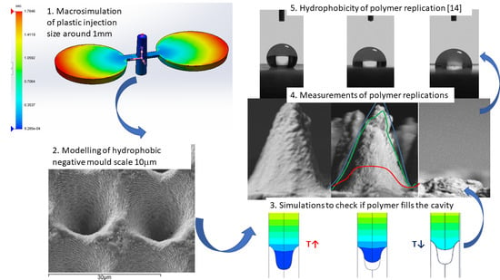
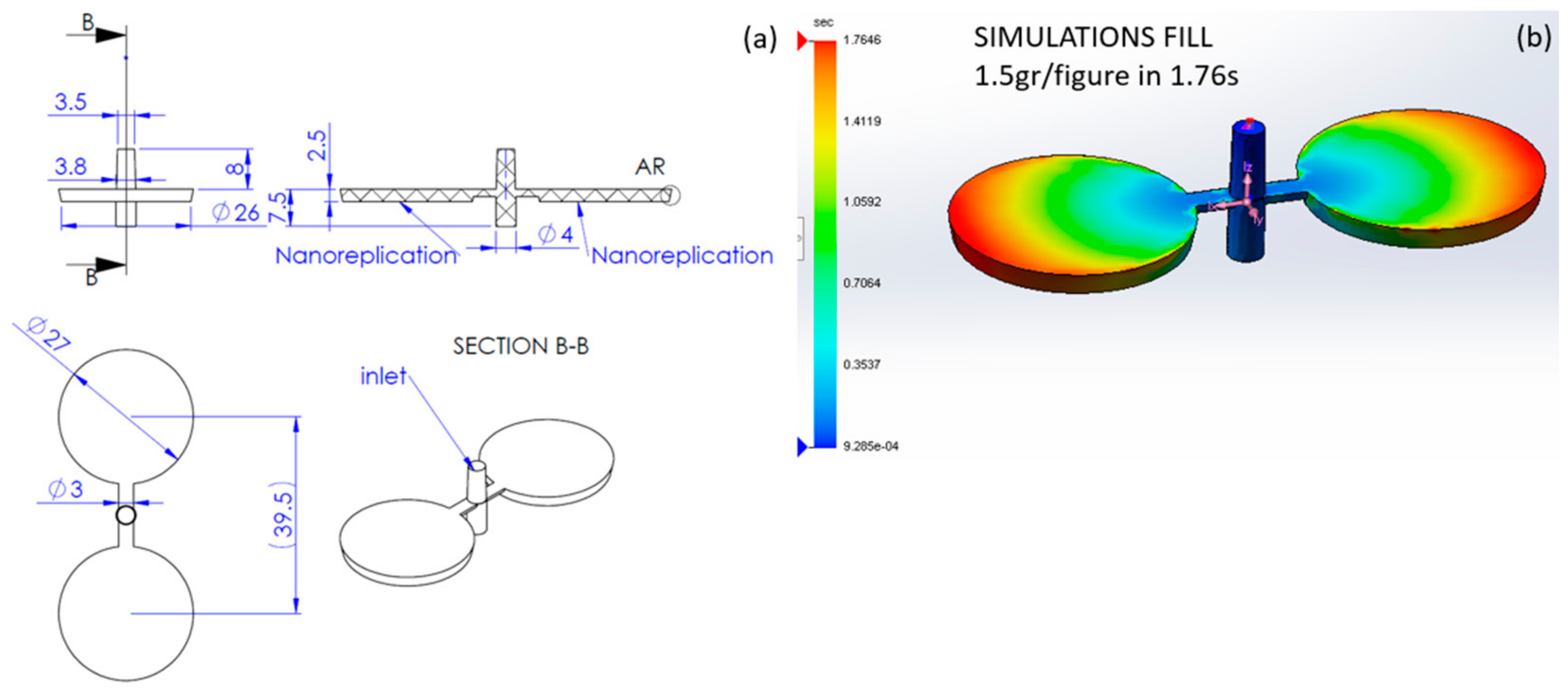
2.4.1. SolidWorks Plastics Macro Simulation
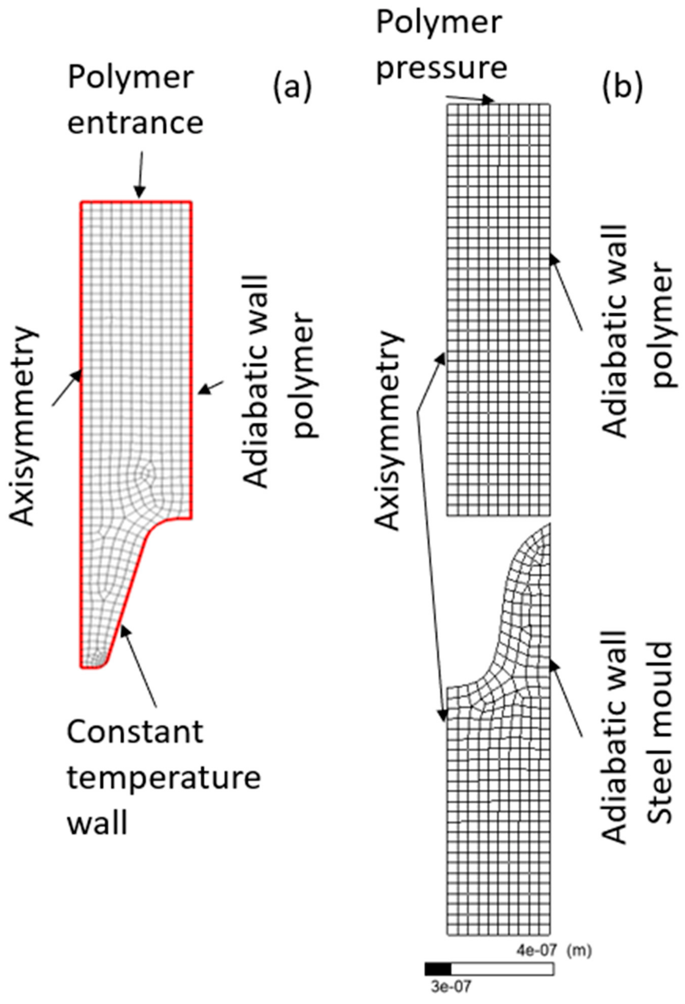
2.4.2. Fluent Approach for Nanoreplication
2.4.3. Polyflow Approach for Nanoreplication
3. Results
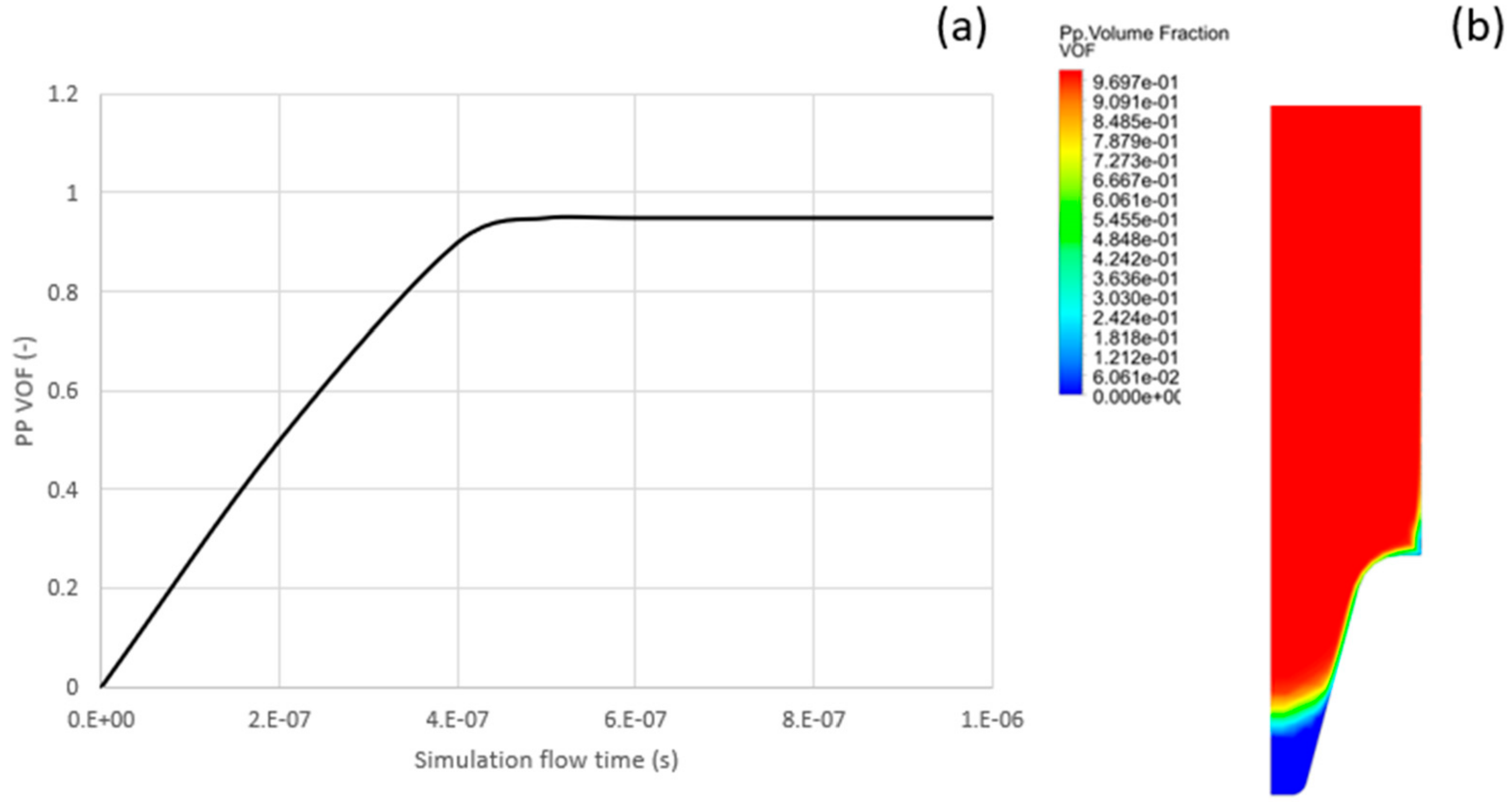
3.1. Fluent
3.2. Polyflow
4. Discussion
5. Conclusions
Supplementary Materials
Author Contributions
Funding
Institutional Review Board Statement
Informed Consent Statement
Data Availability Statement
Conflicts of Interest
References
- Yoo, Y.; Kim, T.; Choi, D.; Hyun, S.; Lee, H.; Lee, K.; Kim, S.; Kim, B.; Seo, Y.; Lee, J.; et al. Injection molding of a nanostructured plate and measurement of its surface properties. Curr. Appl. Phys. 2009, 9, e12–e18. [Google Scholar] [CrossRef]
- Christiansen, A.B.; Clausen, J.S.; Mortensen, N.A.; Kristensen, A. Injection moulding antireflective nanostructures. Microelectron. Eng. 2014, 121, 47–50. [Google Scholar] [CrossRef] [Green Version]
- Kim, S.; Jung, U.T.; Kim, S.; Lee, J.; Choi, H.S.; Kim, C.; Jeong, M.Y. Nanostructured multifunctional surface with antireflective and antimicrobial characteristics. ACS Appl. Mater. Interfaces 2015, 7, 326–331. [Google Scholar] [CrossRef] [PubMed]
- Baruah, S.; Pal, S.K.; Dutta, J. Nanostructured Zinc Oxide for Water Treatment. Nanosci. Nanotechnol. Asia 2012, 2, 90–102. [Google Scholar] [CrossRef] [Green Version]
- Oh, H.J.; Park, J.H.; Lee, S.J.; Kim, B.I.; Song, Y.S.; Youn, J.R. Sustainable fabrication of micro-structured lab-on-a-chip. Lab Chip 2011, 11, 3999–4005. [Google Scholar] [CrossRef] [PubMed]
- Barthlott, W.; Neinhuis, C. Purity of the sacred lotus, or escape from contamination in biological surfaces. Planta 1997, 202, 1–8. [Google Scholar] [CrossRef]
- Yamamoto, M.; Nishikawa, N.; Mayama, H.; Nonomura, Y.; Yokojima, S.; Nakamura, S.; Uchida, K. Theoretical Explanation of the Lotus Effect: Superhydrophobic Property Changes by Removal of Nanostructures from the Surface of a Lotus Leaf. Langmuir 2015, 31, 7355–7363. [Google Scholar] [CrossRef] [PubMed]
- Fagade, A.A.; Kazmer, D.O. Early cost estimation for injection molded components. J. Inject. Molding Technol. 2000, 4, 97–106. [Google Scholar]
- Muntada-López, O.; Pina-Estany, J.; Colominas, C.; Fraxedas, J.; Pérez-Murano, F.; García-Granada, A. Replication of nanoscale surface gratings via injection molding. Micro Nano Eng. 2019, 3, 37–43. [Google Scholar] [CrossRef]
- Pina-Estany, J.; Colominas, C.; Fraxedas, J.; Llobet, J.; Perez-Murano, F.; Puigoriol-Forcada, J.M.; Ruso, D.; Garcia-Granada, A. A statistical analysis of nanocavities replication applied to injection moulding. Int. Commun. Heat Mass Transf. 2017, 81, 131–140. [Google Scholar] [CrossRef] [Green Version]
- Pina-Estany, J.; Granada, A.A.G. 3D Simulation of Nanostructures Replication via Injection Molding. Int. Polym. Process. 2017, 32, 483–488. [Google Scholar] [CrossRef]
- Pina-Estany, J.; Granada, A.A.G. Molecular dynamics simulation method applied to nanocavities replication via injection moulding. Int. Commun. Heat Mass Transf. 2017, 87, 1–5. [Google Scholar] [CrossRef]
- Biosca, A.; Borrós, S.; Clemente, V.P.; Hyre, M.R.; Granada, A.G. Numerical and experimental study of blow and blow for perfume bottles to predict glass thickness and blank mold influence. Int. J. Appl. Glas. Sci. 2019, 10, 569–583. [Google Scholar] [CrossRef]
- Boleda, T.B.; Guardia, C.C.; García-Granada, A.-A. Hydrophobic Hierarchical Structures on Polypropylene by Plastic Injection Molding. 2019. Available online: https://meaagg.com/PLASTFUN/Poster-Nanotoday.pdf (accessed on 2 March 2021).
- Peydró, M.A.; Parres, F.; Crespo, J.E.; Varón, D.J. Study of rheological behavior during the recovery process of high impact polystyrene using cross-WLF model. J. Appl. Polym. Sci. 2010, 120, 2400–2410. [Google Scholar] [CrossRef]
- Anderson, J.D., Jr. Fundamentals of Aerodynamics; Tata McGraw-Hill Education: New York, NY, USA, 2010. [Google Scholar]
- Vasquez, S. A Phase Coupled method for Solving Multiphase Problems on Unstructured Mesh. In Proceedings of the ASME FEDSM’00: ASME 2000 Fluids Engineering Division Summer Meeting, Boston, MA, USA, 11–15 June 2000. [Google Scholar]
- Patankar, S.V. Numerical Heat Transfer and Fluid Flow; CRC Press: Boca Raton, FL, USA, 2018. [Google Scholar]
- Jemcov, A.; Maruszewski, J.P. 12 Algorithm stabilization and acceleration in computational fluid dynamics: Exploiting recursive properties of fixed point algorithms. Comput. Fluid Dyn. Heat Transf. Emerg. Top. 2011, 23, 459. [Google Scholar]
- Choudhary, M.K.; Venuturumilli, R.; Hyre, M.R. Mathematical Modeling of Flow and Heat Transfer Phenomena in Glass Melting, Delivery, and Forming Processes. Int. J. Appl. Glas. Sci. 2010, 1, 188–214. [Google Scholar] [CrossRef]
- Chouffart, Q. Experimental and Numerical Investigation of the Continuous Glass Fiber Drawing Process; Université de Liège: Liège, Belgium, 2018. [Google Scholar]
- Loaldi, D.; Regi, F.; Baruffi, F.; Calaon, M.; Quagliotti, D.; Zhang, Y.; Tosello, G. Experimental Validation of Injection Molding Simulations of 3D Microparts and Microstructured Components Using Virtual Design of Experiments and Multi-Scale Modeling. Micromachines 2020, 11, 614. [Google Scholar] [CrossRef] [PubMed]


| ρ (kg/m3) | α (W/(m K)) | k (J/kg K) | |
|---|---|---|---|
| Steel mold | 7800 | 20 | 460 |
| PP polymer | 850 | 0.15 | 3100 |
| D1 (Pa·s) | D2 (K) | D31 (K/Pa) | A1 (-) | A3 (K) | τ (Pa) | n (-) | T*1 (K) | A21 (K) |
|---|---|---|---|---|---|---|---|---|
| 7.4 × 1031 | 113.15 | 0 | 32.7 | 51.6 | 26,260 | 0.272 | 113.15 | 51.6 |
| A1 (log(Pa s)) | B1 (K*log(Pa s)) | T0 (K) |
|---|---|---|
| 0.2 | 1110 | 113.15 |
| CPU Time (s) | Simulated Time (s) | Mesh Size (mm) | Nodes (-) | Time Step (s) | Hard Disk Required (MB) | |
|---|---|---|---|---|---|---|
| SolidWorks Plastics | 1320 | 50 | 1 | 10,500 | 0.012 1 | 93 |
| Ansys Fluent | 43,200 | 1 × 10⁻⁶ | 0.001 | 1092 | 1 × 10⁻¹⁵ | 80,000 2 |
| Ansys Polyflow | 600 | 15 | 0.001 | 813 | 5 × 10⁻³ | 534 |
Publisher’s Note: MDPI stays neutral with regard to jurisdictional claims in published maps and institutional affiliations. |
© 2021 by the authors. Licensee MDPI, Basel, Switzerland. This article is an open access article distributed under the terms and conditions of the Creative Commons Attribution (CC BY) license (https://creativecommons.org/licenses/by/4.0/).
Share and Cite
Baldi-Boleda, T.; Sadeghi, E.; Colominas, C.; García-Granada, A. Simulation Approach for Hydrophobicity Replication via Injection Molding. Polymers 2021, 13, 2069. https://doi.org/10.3390/polym13132069
Baldi-Boleda T, Sadeghi E, Colominas C, García-Granada A. Simulation Approach for Hydrophobicity Replication via Injection Molding. Polymers. 2021; 13(13):2069. https://doi.org/10.3390/polym13132069
Chicago/Turabian StyleBaldi-Boleda, Tomás, Ehsan Sadeghi, Carles Colominas, and Andrés García-Granada. 2021. "Simulation Approach for Hydrophobicity Replication via Injection Molding" Polymers 13, no. 13: 2069. https://doi.org/10.3390/polym13132069
APA StyleBaldi-Boleda, T., Sadeghi, E., Colominas, C., & García-Granada, A. (2021). Simulation Approach for Hydrophobicity Replication via Injection Molding. Polymers, 13(13), 2069. https://doi.org/10.3390/polym13132069