1. Introduction
The imbalance of polymer flow in geometrically balanced multi-cavity injection molds is a serious and difficult to handle problem in the injection molding process. This phenomenon may be observed in H-type runner layouts, which are depicted in
Figure 1. At present, it is established that the imbalance results from the polymer melt flow shear gradients developed in the runner system, which in turn lead to non-symmetrical temperature and viscosity distributions. This is influenced and complicated by the runner’s geometry, thermo-rheological material characteristics, and injection molding process parameters [
1,
2,
3,
4,
5,
6,
7].
The imbalance phenomenon has been investigated extensively for years by scientists and engineers [
1,
2,
3,
4,
5,
6,
7,
8,
9,
10,
11,
12,
13,
14,
15,
16,
17,
18,
19,
20,
21,
22,
23,
24,
25]. However, there is not any commonly accepted procedure for problem solving. A detailed discussion of the literature review has been recently presented by the authors of this paper [
1,
2]. This review is summarized below.
The fundamental research was carried out by Beaumont and his co-workers [
3,
4,
5,
6] as well as by Reifschneider [
7] who tried to explain the phenomenon of filling imbalance. Beaumont et al. developed the commercial technique called melt rotation technology to diminish the filling imbalance [
3,
4,
5,
6]. In addition to the basic design with one correction element, double corrections and a circular element were proposed. However, these designs were not studied by simulation or experimentation. Another approach has been proposed by Huang [
8], who applied profiled channels instead of straight channels.
Petzold [
9] and Fernandes [
10] developed the concepts of optimizing the temperature field of the flowing polymer. Rhee [
11,
12] proposed flow balancing by using the throttle valves in the runners which were activated when the mold temperature rises. Schwenk [
13] studied the effect of mold venting on flow balancing.
Recently, the filling imbalance has been investigated with advanced techniques. Gim et al. [
14] used a mold equipped with thermocouples and in-direct pressure sensors, and they observed that the filling imbalance may be inverse. Li et al. [
15] studied the phenomenon by direct in-mold observations using a mold with a sight glass.
The mold filling simulation software [
16,
17,
18,
19] was not able to diagnose the shear effect on the polymer flow for a long time. The use of simple 1D beam elements, and 2D or 2.5D approach did not allow to predict the shear phenomena properly. Thus, new simulation concepts have been proposed to study the problem [
20,
21]. These included three-dimensional non-isothermal non-Newtonian flow and inertia effects. Convection was predicted using 3D velocity vector, and this allowed the simulation of the temperature field around the runners properly. Moreover, a flexible meshing was applied to provide high-resolution mesh for the runners and the cavity. Several simulation studies have confirmed this approach [
22,
23,
24,
25].
Summarizing, so far, the filling imbalance has been studied experimentally and to a less extent by simulation for geometrically balanced systems and for basic melt rotation solutions only.
Recently, extensive experimental and simulation studies on the filling imbalance have been performed by the authors of this paper [
1,
2]. Balancing the polymer flow between cavities has been investigated at various operating conditions using various runner systems, which are depicted in
Figure 2. The experiments indicated that the process parameters: injection rate, mold and melt temperature as well as the runners’ layout geometry significantly affect the filling imbalance. However, the imbalance has never been eliminated completely. A special simulation technique was developed to simulate the phenomenon properly, including inertia effects and 3D tetrahedron meshing of at least 12 layers as well as meshing of the nozzle. It has been concluded that the thermo-rheological characteristics of the material, defined by the parameters of the Cross-WLF model, i.e., the index flow, critical shear stress (relaxation time), and zero shear viscosity, as well as characterized by the thermal diffusivity and heat transfer coefficient, significantly affect the filling imbalance. This is strongly dependent on the runners’ layout geometry and process operating conditions: flow rate and shear rate. The main conclusion of these studies was that there is no universal procedure to overcome the filling imbalance, and the only reasonable approach is to optimize the process parameters (material parameters, operating conditions, as well as runners’ geometry and layout) for the currently implemented process.
In this paper, a novel optimization approach has been presented to solve the filling imbalance problem. Three optimization procedures were applied: Response Surface Method (RSM), Taguchi procedure, and Artificial Neural Networks (ANN).
2. Optimization Window
The phenomenon was studied both by simulation and experimentation using several different runner systems at various thermo-rheological material parameters and process operating conditions. Operating process parameters of the injection rate
Vinj, melt temperature
Tm, and mold temperature
TM, as well as the geometry of the runner system were optimized, i.e., these were the optimized process parameters. The imbalance of the mold filling
Im as well as the process parameters of injection pressure
Pinj, injection time
tinj, and molding temperature
Tmolding were the optimization criteria (
Table 1).
Studies have been performed for an eight-cavity injection mold of “H-type” runner layout equipped with inserts of different geometry. A standard geometry GS have been used as well as three overturn geometries, G1 with one correction element, G2 with two correction elements, and G3 with circled element, these are depicted in
Figure 2.
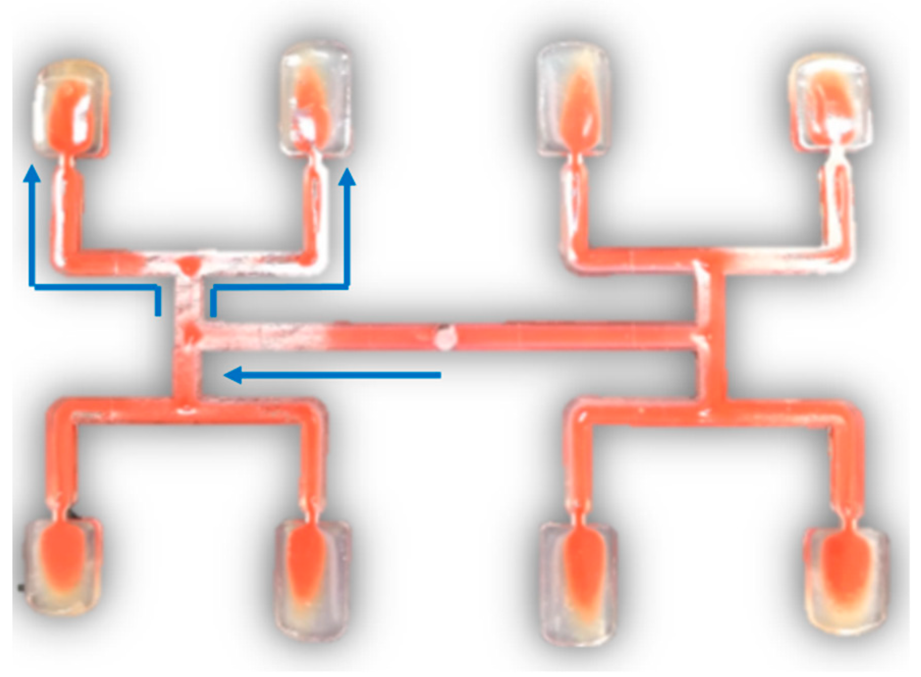
The factor of mass filling imbalance
Im [
2] has been applied to evaluate the degree of imbalance which is defined as
where
Im is the factor of mass filling imbalance,
m1 is the mass of polymer from the inner cavities, and
m2 is the mass of polymer from the outer cavities (
Figure 3).
The imbalance factor is positive when the inner cavities (1) fills faster (Im > 0), and it is negative when the outer cavities (2) filled faster (Im < 0).
The optimization criteria determine the global objective function which was defined in the following way:
where
F is the global objective function,
i is the number of optimization criteria,
wi is the weight of the
i-criterion,
fi is the value of the normalized
i-criterion.
The optimization criteria were specified as follows: f1 is the filling imbalance Im, f2 is the injection pressure Pinj, f3 is the injection time tinj, and f4 is the molding temperature Tmolding.
The values of the weights were as follows:
w1 = 0.5 for the filling imbalance
Im,
w2 = 0.1 for the injection pressure
Pinj,
w3 = 0.2 for the injection time
tinj, and
w4 = 0.2 for the molding temperature
Tmolding. These are summarized in
Table 2.
The optimization criteria were normalized in the following way:
- -
when the optimization criterion is the minimum value of the output variable
yi:
- -
when the optimization criterion is the maximum value of the output variable
yi:
3. Optimization Procedures
Three optimization procedures were applied: Response Surface Methodology (RSM), Taguchi Method, and Brain Construction Algorithm (BCA) developed by STASA, which are shortly characterized below.
Response Surface Methodology (RSM) is a widely known and recognized statistical optimization method that explores the relationships between several input variables (independent variables) and one or more output variables (dependent or response variables) [
26,
27,
28]. The main idea of RSM is to use a sequence of designed experiments to obtain an optimal response. However, a full factorial design is used in RSM, which means considering all combinations of parameter interactions, and it is time-consuming.
The RSM procedure consists of a full factorial experiment, approximation of the experimentation results (to do this, using a second-degree polynomial model is suggested), development of an extended set of data (to densify the response surface), and data normalization and selection based on the global objective function.
The Taguchi method [
29,
30] is based on the orthogonal array experiments, which provides much reduced variance for the study with an optimum setting of process control parameters. Thus, the integration of design of experiments (DOE) with parametric optimization of process to obtain desired results is achieved in the Taguchi method. Many experiments must be performed when the number of control factors is high. Taguchi methods use a special design of orthogonal arrays to study the entire factor space with only a small number of experiments.
The Taguchi method uses the signal-to-noise (S/N) ratio instead of the average value to convert the trial result data into a value for the characteristic in the optimum setting analysis. The S/N ratio reflects both the average and the variation of the quality characteristic.
The standard S/N ratios generally used are as follows: nominal is best (NB), lower the better (LB), and higher the better (HB). The larger (higher) the better type characteristic (HB) is applied for problems where maximization of the quality characteristic of interest is sought. The smaller (lower) the better type characteristic (LB) is applied for problems where minimization of the characteristic is intended. The nominal the best characteristic (NB) is used for problems where one tries to minimize the mean squared error around a specific target value.
Brain Construction Algorithm (BCA) is based on self-generating neural networks developed by STASA [
31,
32] that are linked with classical statistics. This has the flexibility and universality of neural models and the transparency of statistical theory. STASA has implemented a D-optimal design routine that tries to maximize the parameter space with a minimum of experiments. The result is an optimally adapted experimental design.
This novel optimization approach is based on the combination of mold filling numerical simulation and the BCA procedure implemented in the STASA QC software.
The procedure starts with the definition of optimization parameters and quality features (optimization criteria). Besides continuous measurable quality features such as dimensions or weight, also, attributive features that are evaluated in a more subjective way, e.g., surface glance, can be defined.
In the next step, the software provides a design of experiment that is automatically created based on the parameters’ definitions. The experimental design provides a table with different parameter settings, which have to be set on the simulation consecutively. At every setting, the quality features of the simulated parts have to be measured. With this experimental design, the user receives guidance how to change the process setting systematically to receive the information about the interrelations between parameters and quality features required to generate the models.
In practice, the number of experiments (different machine settings) in the experimental design is limited by cost factors. In general, no more than about 10 to 20 different machine settings are acceptable in practical applications. That is the reason the numerical calculation have been utilized. In spite of that, taking into account a full factorial design used in RSM, which means considering all combinations of parameter interactions, can only be used in exceptional cases.
4. Optimization Results
4.1. Optimization by Response Surface Methodology (RSM)
The results of optimizations performed by RSM method are depicted in
Figure 4 and
Figure 5. Simulation and experimental results for optimum set of data are presented in
Figure 6.
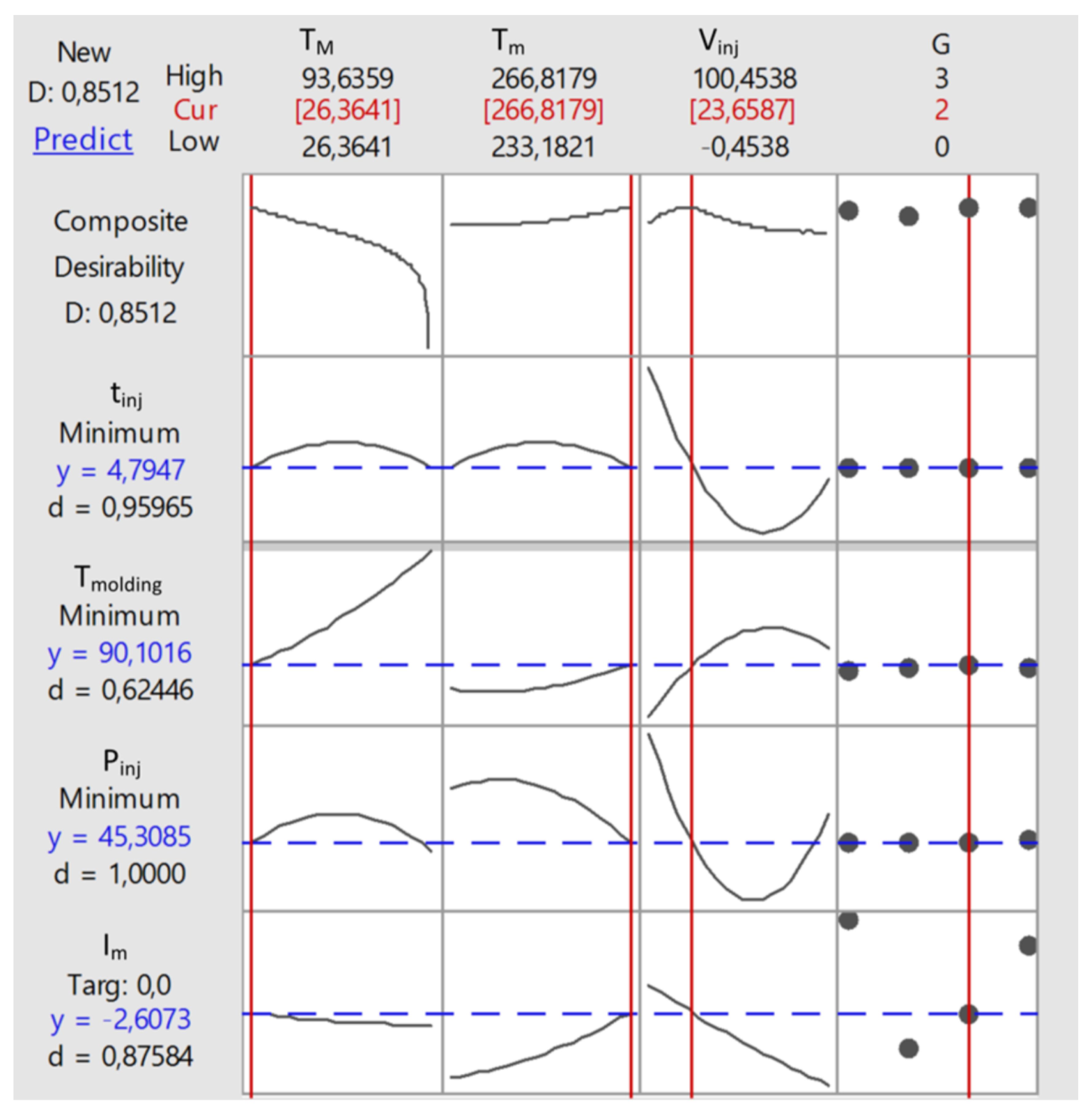
Figure 4 shows the optimum values of process parameters: the mold temperature
TM, the melt temperature
Tm, the injection rate
Vinj, as well as the geometry of the runner system
G, which are marked in red. The graphs show the optimum solution (red line) against the background of the desirability function (objective function). The optimum values of process parameters are listed in the conclusion table (Table 5).
The composite (global) desirability dependence on each of the optimized parameters with the fixed (optimum) values of the other three parameters is presented in the first line. For example, the first graph from the left shows the dependence of the composite desirability
D on the mold temperature
TM at constant values of other parameters, i.e
.,The individual desirability functions are shown in the next four lines with the values of these for the optimum set of data, i.e.,
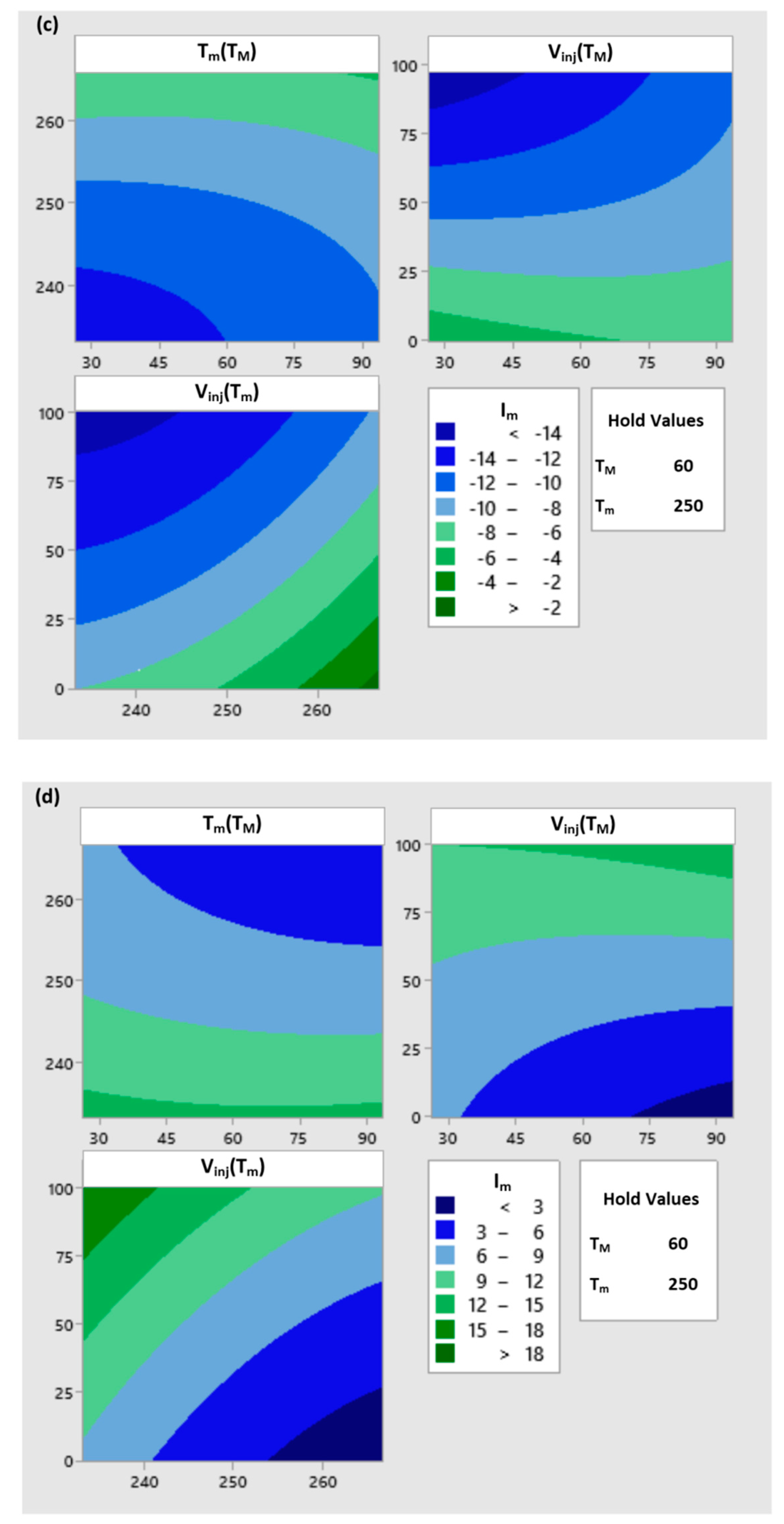
Figure 5 presents the dependence (by regression) of the filling imbalance
Im (output parameter) on each pair of two of the four input parameters (
TM,
Tm,
Vinj,
G) with fixed values (center of the variation range) of the other two parameters. For example, the graph in the upper left corner shows the dependence of the filling imbalance
Im on the mold temperature
TM and the melt temperature
Tm at the constant values
Vinj = 50 mm/s and
G = 0.
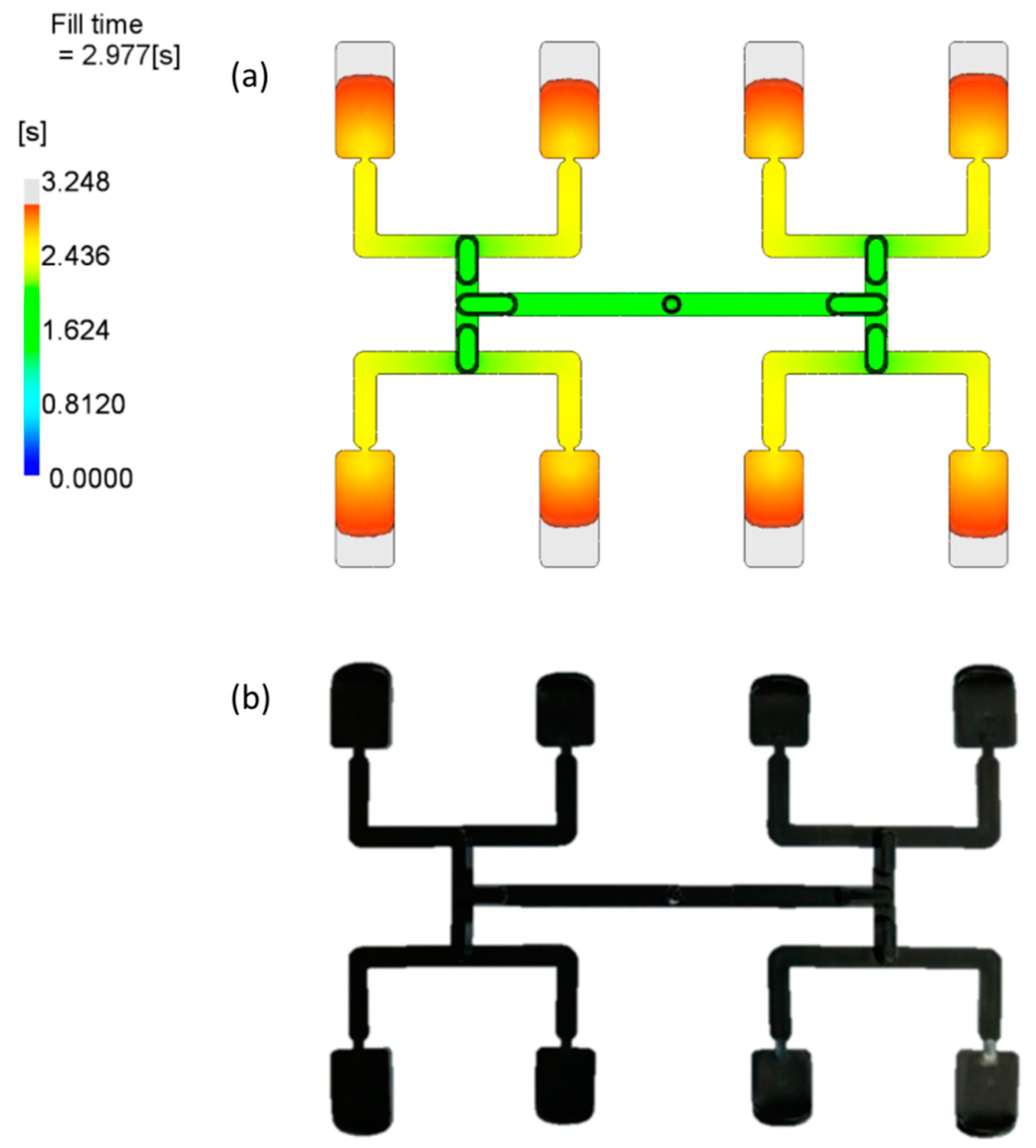
Figure 6 presents simulation and experimental results for optimum set of data. It is clearly seen that the imbalance is relatively low, and equal to about
Im = −9%, which means the outer cavities are filled faster.
4.2. Optimization by Taguchi Method
The Taguchi method implemented into the Moldex3D software has some limitations. The optimization window is defined by the limited number of optimized parameters. For that reason, we assumed (from the available data) the following parameters (control factors, optimized parameters): the mold temperature
TM, the melt temperature
Tm, the filling time
tfill, and the mesh size
M. In this approach, the filling time
tfill corresponds to the injection rate
Vinj, and the mesh size
M corresponds to the runner geometry
G. The range of these data is presented in
Table 3.
The optimization criteria (quality factors) are also limited, and were selected as follows: the density distribution
Ddistrib, the average temperature distribution
Tav, and the sprue injection value
Psprue. These factors correspond to the filling imbalance
Im, the molding temperature
Tmolding, and the injection pressure
Pinj. The characteristics of these and their weighting is presented in
Table 4.
The optimal setting is the parameters combination that has the highest S/N ratio. For example, the filling time has the highest S/N ratio for the set of control factors (optimized parameters) defined by Level 4 (
Figure 7).
In the paper,
smaller the better characteristic has been used for the average temperature distribution
Tav and the sprue injection pressure
Psprue, and
nominal the best characteristic for the density distribution
Ddistrib (
Table 4).
The results of optimizations performed by Taguchi method are depicted in
Figure 7 and
Figure 8. Simulation and experimental results for optimum set of data are presented in
Figure 9.
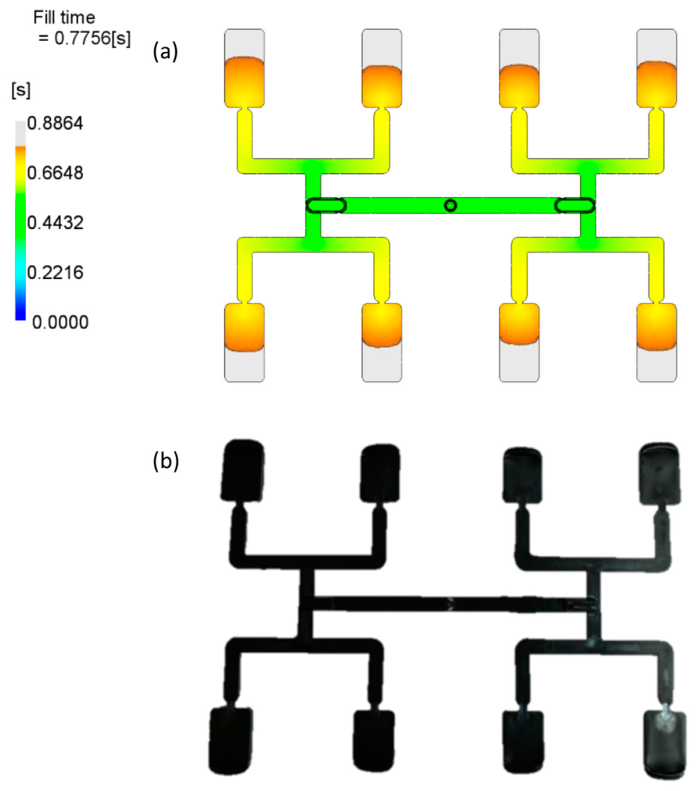
Figure 9 presents simulation and experimental results for optimum set of data. It is clearly seen that the imbalance is relatively low, and equal to about
Im = −14%, which means the outer cavities are filled faster.
4.3. Optimization by Neural Network STASA
The results of optimizations performed by STASA software are depicted in
Figure 10 and
Figure 11. Simulation and experimental results for optimum set of data are presented in
Figure 12.
Figure 10 shows the optimum values of process parameters: the mold temperature
TM, the melt temperature
Tm, the injection rate
Vinj, as well as the geometry of the runner system
G, which are equal to:
TM = 40 °C,
Tm = 257 °C,
Vinj = 68 mm/s,
G = 1, respectively. The optimum is described by the red line that connects the optimal parameter values.
The optimum values of process parameters are listed in the conclusion table (
Table 5).
The values of optimization criteria for optimal setting with respect to the predefined range of searching are presented in
Figure 11. The red dots indicate the values of the criteria, the black dots represent the predefined target values, and the green areas represent the range of searching.
Figure 12 presents simulation and experimental results for optimum set of data. It is clearly seen that the imbalance is relatively low, and equal to about I
m = −9%, which means the outer cavities are filled faster.
5. Discussion
The optimization results are summarized in
Table 5. The optimal values of process parameters (
Vinj,
Tm, TM, G) and the corresponding values of optimization criteria (
Im,
Pinj,
tinj,
Tmolding), as well as the values of global objective function
F are given. The simulation results were obtained using Moldflow software, the prediction results were received from optimization software by calculation on the base of their own models built on the simulation data. The experimental results were obtained by performing the experiment at the optimal process parameters.
The highest value of the global objective function has been predicted for the optimal process parameters indicated by BCA method (STASA QC), and also for these optimal parameters, the highest value of the experimental global objective function has been obtained. So, it seems to be justified that the Artificial Neural Networks approach is the most efficient optimization procedure, and the Brain Construction Algorithm (BCA) might be proposed for problem solving of imbalance phenomena.
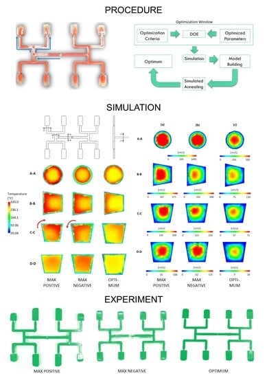
However, it is important to note that all the optimization procedures substantially improved the filling balance, which is also confirmed by simulations depicted in
Figure 13 and
Figure 14.
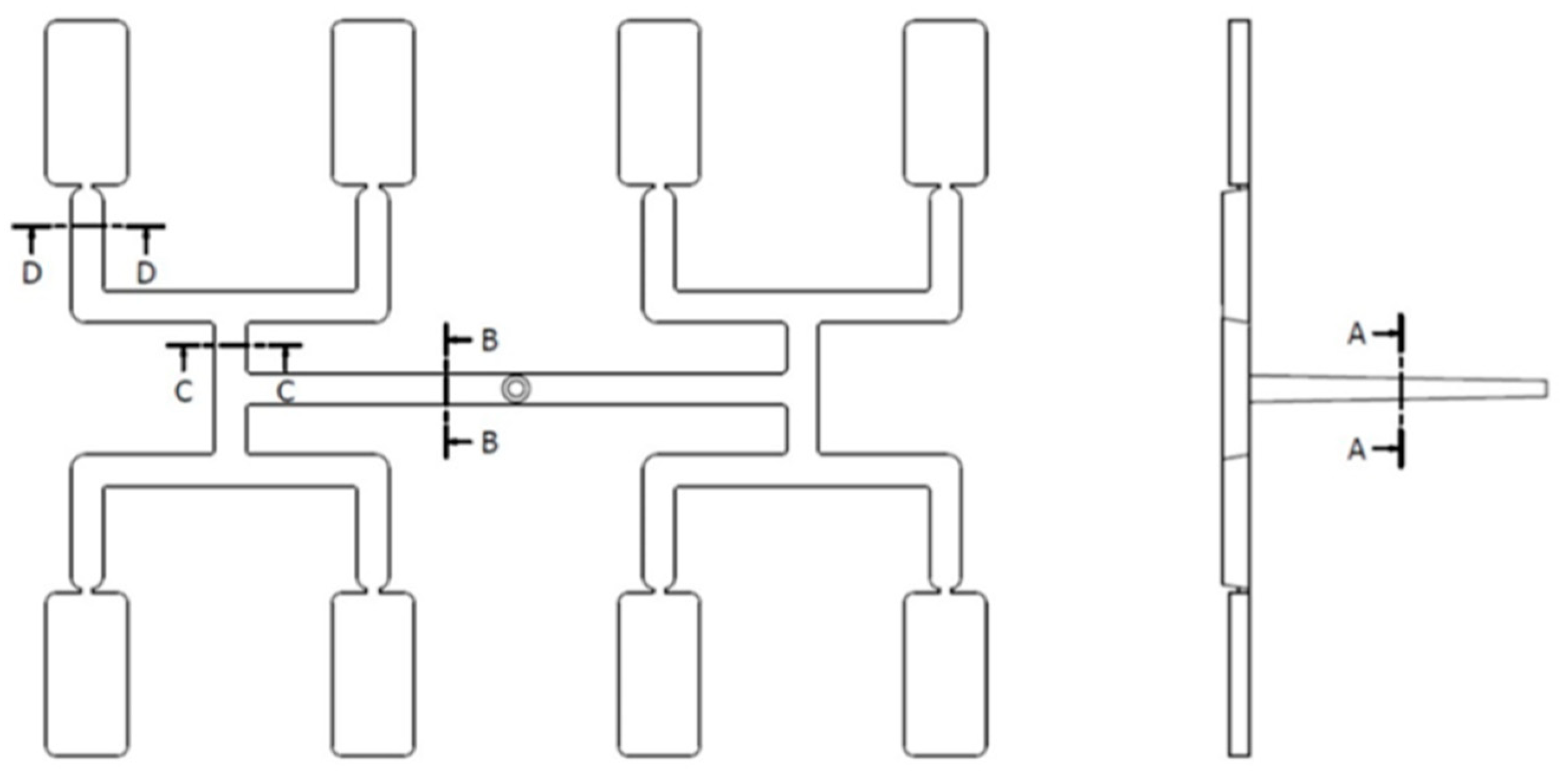
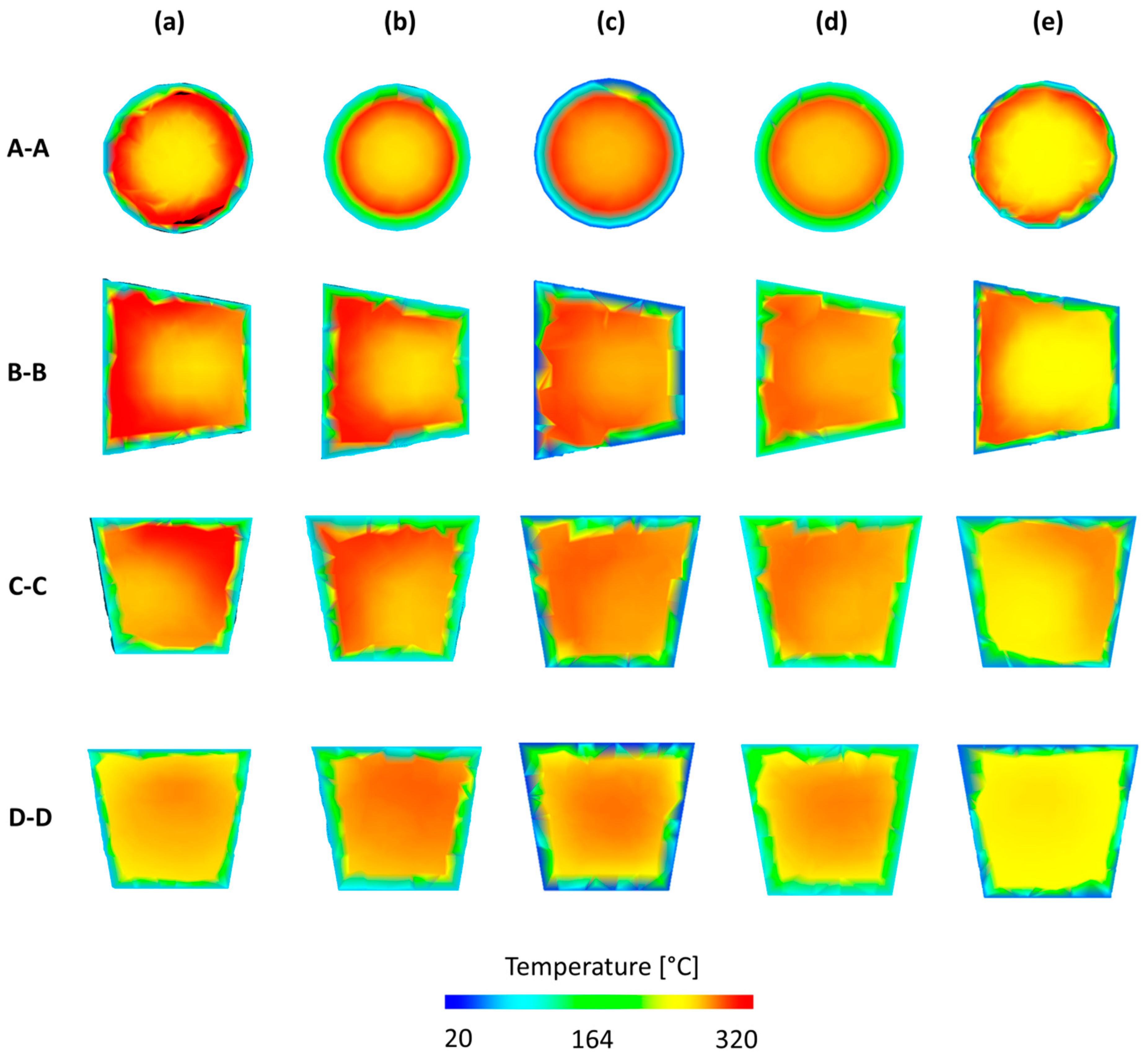
Temperature plots in specific cross-sections of the standard runner system (
Figure 13) obtained from simulations performed on different data, and using different optimization procedures are depicted in
Figure 14. A maximum positive imbalance and maximum negative imbalance, as well as optimum data for RSM, Taguchi, and STASA are shown. It is clearly seen that for the standard geometry
GS, the polymer melt stream rotates to the right (cross-section C–C,
Figure 14a), which results in a positive imbalance. While, for the two overturn geometry
G2 the polymer melt stream rotates to the left (cross-section C–C,
Figure 14b), which results in a negative imbalance. In the optimized cases, there is no substantial melt stream rotation that leads to much more balanced flow and cavity filling. It is worth noting that rotation is observed in all cases; however, the degree of rotation varies.
Velocity plots in specific cross-sections of the runner system (
Figure 13) obtained from simulations performed on the data providing a maximum positive imbalance and maximum negative imbalance as well as optimum data for STASA system are depicted in
Figure 15. The most balanced flow is clearly seen for the data indicated by STASA (
Figure 15c).
The comparison is related to the simulation validation, not to the optimization. An accuracy of simulation is quite good, especially in the case of BCM procedure. In this case, the optimized value of injection rate
Vinj was very high. It results from our previous studies that discrepancies between simulation and experimentation data substantially increase when injection rate
Vinj increases [
1].
6. Conclusions
Three optimization techniques were used to study and optimize the filling imbalance in geometrically balanced injection molds: Response Surface Methodology (RSM), Taguchi method, and Artificial Neural Networks (ANN). The process parameters of injection rate Vinj, melt temperature Tm, and mold temperature TM, as well as the geometry of the runner system G were optimized. The mold filling imbalance Im as well as the process parameters of injection pressure Pinj, injection time tinj, and molding temperature Tmolding were the optimization criteria.
It can be concluded that using the optimization procedures improves the filling imbalance; however, the Artificial Neural Networks using the Brain Construction Algorithm (BCA) seems to be the most efficient optimization procedure.
It can be also noted that a comprehensive approach to modeling of injection molding may be useful for simulation of the flow in injection molds and for the prediction of the filling imbalance. A global injection molding model might be considered for simulation of the polymer melt flow in the plasticating unit of the injection molding machine as well as in the mold. Resulting parameters of the plasticating unit simulations would be input data for the mold flow simulations. Some of the injection molding studies with this respect were recently discussed by the authors [
1,
2].


