Mathematical Analysis of Pseudoplastic Polymers during Reverse Roll-Coating


Abstract

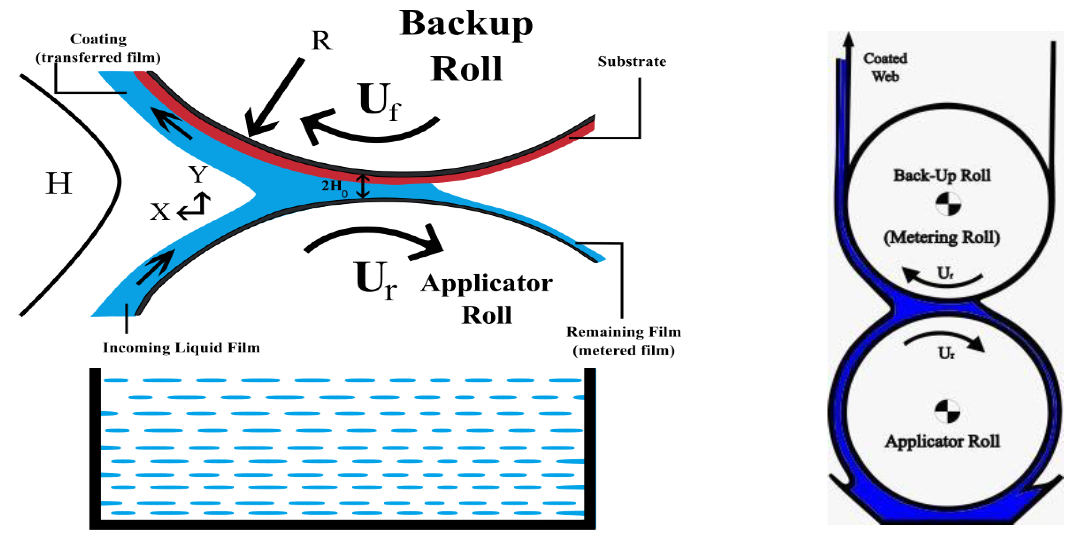
1. Introduction
2. Mathematical Formulation
3. The Dimensionless Form
4. Solution of the Problem
4.1. Zeroth-Order Solution
4.2. First-Order Solution
5. Operating Variables
5.1. Separating Force
5.2. Power Input
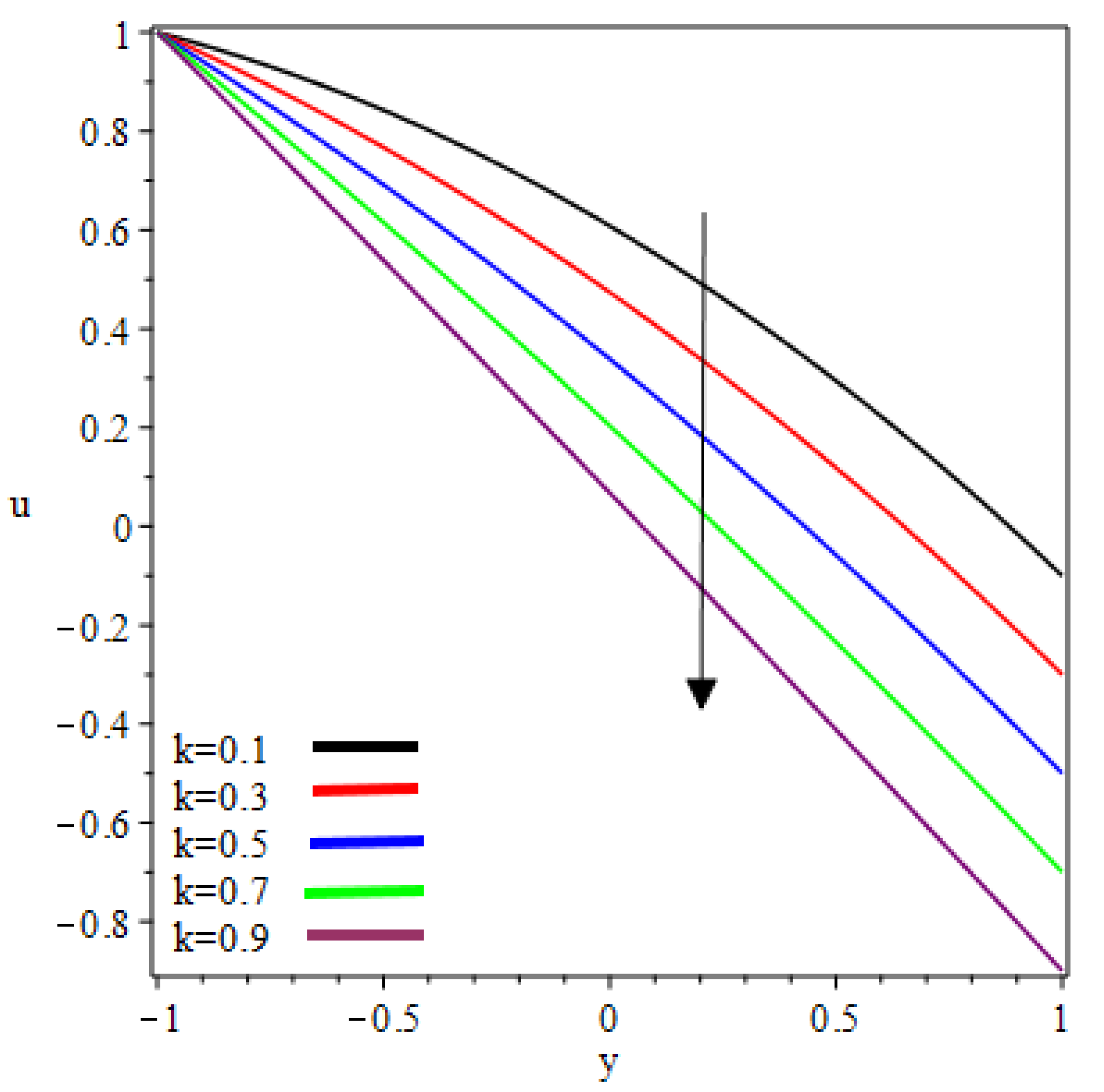
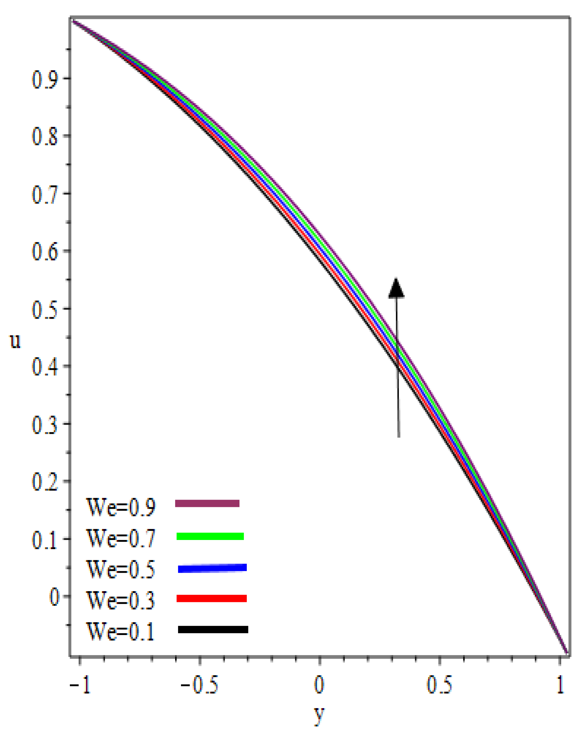
6. Results and Discussion
7. Conclusions
- ➢
- Flow velocity increases as increases.
- ➢
- Maximum velocity occurs at the roll surface of the reverse roll.
- ➢
- Absolute pressure gradient is maximum at the nip point.
- ➢
- Viscous forces are dominant over the elastic forces.
- ➢
- Concavity of the pressure distribution changes in the interval .
- ➢
- The velocity ratio parameters and Weissenberg number play important roles in controlling the pressure gradient and pressure distribution.
- ➢
- The Weissenberg number provides an economical mechanism to control the magnitude of separation force and power input.
- ➢
- The Weissenberg number also plays fundamental role to have flow rate, separation points and coating thickness as per desirous.
- ➢
- Pressure distribution, power input and the viscous forces play a significant role in coating thickness.
- ➢
- As a fluid moves to the separation point of reverse roll-coating, the viscosity of the fluid increases and the coating of the web is done after this position.
- ➢
- If , the results of [13] are recovered.
8. Future Work
Author Contributions
Funding
Conflicts of Interest
Abbreviations
| Peripheral velocity of the reverse roll | |
| Peripheral velocity of forwarding roll | |
| Radius of the roll | |
| Velocities ratio | |
| Extra stress tensor | |
| Density | |
| Share rate | |
| Second invariant strain tensor | |
| Weissenberg number | |
| Half the nip separation | |
| Thickness of the coating on reverse roll | |
| Thickness of the coating on the forwarding roll | |
| Coating Thickness | |
| Ratio of the half of the nip region to the coating thickness on the reverse roll | |
| Dimensionless flow rate |
References
- Balzarotti, F.; Rosen, M. Systematic study of coating systems with two rotating rolls. Lat. Am. Appl. Res. 2009, 39, 99–104. [Google Scholar]
- Belblidia, F.; Tamaddon-Jahromi, H.R.; Echendu, S.O.S.; Webster, M.F. Reverse roll-coating flow: A computational investigation towards high-speed defect free coating. Mech. Time Depend. Mater. 2013, 17, 557–579. [Google Scholar] [CrossRef]
- Zafar, M.; Rana, M.A.; Zahid, M.; Malik, M.A.; Lodhi, M.S. Mathematical Analysis of Roll Coating Process by Using Couple Stress Fluid. J. Nanofluids 2019, 8, 1683–1691. [Google Scholar] [CrossRef]
- Zheng, G.; Wachter, F.; Al-Zoubi, A.; Durst, F.; Taemmerich, R.; Stietenroth, M.; Pircher, P. Computations of coating windows for reverse roll coating of liquid films. J. Coat. Technol. Res. 2020. [Google Scholar] [CrossRef]
- Benkreira, H.; Edwards, M.F.; Wilkinson, W.L. A semi-empirical model of the forward roll coating flow of newtonian fluids. Chem. Eng. Sci. 1981, 36, 423–427. [Google Scholar] [CrossRef]
- Jang, J.Y.; Chen, P.Y. Reverse roll coating flow with non-Newtonian Fluids. Commun. Comput. Phys. 2009, 6, 536–552. [Google Scholar]
- Hao, Y.; Haber, S. Reverse roll coating flow. Int. J. Numer. Methods Fluids 1999, 30, 635–652. [Google Scholar] [CrossRef]
- Benkreira, H.; Edwards, M.F.; Wilkinson, W.L. Roll coating of purely viscous liquids. Chem. Eng. Sci. 1981, 36, 429–434. [Google Scholar] [CrossRef]
- Greener, J.; Middleman, S. Theoretical and experimental studies of the fluid dynamics of a two-roll coater. Ind. Eng. Chem. Fundam. 1979, 18, 35–41. [Google Scholar] [CrossRef]
- Coyle, D.J.; Macosko, C.W.; Scriven, L.E. The fluid dynamics of reverse roll coating. Aiche J. 1990, 36, 161–174. [Google Scholar] [CrossRef]
- Taylor, J.; Zettlemoyer, A. Hypothesis on the mechanism of ink splitting during printing. Tappi J. 1958, 12, 749–757. [Google Scholar]
- Hintermaier, J.; White, R. The splitting of a water film between rotating rolls. Tappi J. 1965, 48, 617–625. [Google Scholar]
- Greener, J.; Middleman, S. Reverse roll coating of viscous and viscoelastic liquids. Ind. Eng. Chem. Fundam. 1981, 20, 63–66. [Google Scholar] [CrossRef]
- Ho, W.S.; Holland, F.A. Between-rolls metering coating technique. Tappi J. 1978, 61, 53–56. [Google Scholar]
- Shiode, H.; Tamai, H.; Isaki, T. Flow Simulations of Dynamic Wetting Line at a Reverse-roll Coater Using the VOF Method. Nihon Reoroji Gakkaishi 2009, 37, 59–64. [Google Scholar] [CrossRef]
- Zahid, M.; Rana, M.A.; Siddiqui, A.M. Roll coating analysis of a second-grade material. J. Plast. Film Sheeting 2017, 34, 232–255. [Google Scholar] [CrossRef]
- M, Z.; Zafar, M.; Rana, M.A.; Rana, M.; Lodhi, M.S. Numerical analysis of the forward roll coating of a rabinowitsch fluid. J. Plast. Film Sheeting 2019, 36, 191–208. [Google Scholar] [CrossRef]
- Khandavalli, S.; Rothstein, J.P. Ink transfer of non-Newtonian fluids from an idealized gravure cell: The effect of shear and extensional deformation. J. Non Newton. Fluid Mech. 2017, 243, 16–26. [Google Scholar] [CrossRef]
- Khan, M.I.; Alzahrani, F.; Hobiny, A.; Ali, Z. Fully developed second order velocity slip Darcy-Forchheimer flow by a variable thicked surface of disk with entropy generation. Int. Commun. Heat Mass Transf. 2020, 117, 104778. [Google Scholar] [CrossRef]
- Wang, J.; Muhammad, R.; Khan, M.I.; Khan, W.A.; Abbas, S.Z. Entropy optimized MHD nanomaterial flow subject to variable thicked surface. Comput. Methods Programs Biomed. 2020, 189, 105311. [Google Scholar] [CrossRef]
- Khan, M.I.; Alzahrani, F.; Hobiny, A. Heat transport and nonlinear mixed convective nanomaterial slip flow of Walter-B fluid containing gyrotactic microorganisms. Alex. Eng. J. 2020. [Google Scholar] [CrossRef]
- Wang, J.; Khan, M.I.; Khan, W.; Abbas, S.Z.; Khan, M.I. Transportation of heat generation/absorption and radiative heat flux in homogeneous—Heterogeneous catalytic reactions of non-Newtonian fluid (Oldroyd-B model). Comput. Methods Programs Biomed. 2020, 189, 105310. [Google Scholar] [CrossRef] [PubMed]
- Zafar, M.; Rana, M.A.; Zahid, M.; Ahmad, B. Mathematical Analysis of the Coating Process over a Porous Web Lubricated with Upper-Convected Maxwell Fluid. Coatings 2019, 9, 458. [Google Scholar] [CrossRef]
- Lyubimov, D.V.; Perminov, A.V. Motion of a thin oblique layer of a pseudoplastic fluid. J. Eng. Phys. Thermophys. 2002, 75, 920–924. [Google Scholar] [CrossRef]
- Williamson, R.V. The flow of pseudoplastic materials. Ind. Eng. Chem. 1929, 21, 1108–1111. [Google Scholar] [CrossRef]
- Nadeem, S.; Akbar, N.S. Numerical solutions of peristaltic flow of williamson fluid with radially varying mhd in an endoscope. Int. J. Numer. Methods Fluids 2011, 66, 212–220. [Google Scholar] [CrossRef]
- Cramer, S.D.; Marchello, J.M. Numerical evaluation of models describing non-Newtonian behavior. Aiche J. 1968, 14, 980–983. [Google Scholar] [CrossRef]
- Dapra, I.; Scarpi, G. Perturbation solution for pulsatile flow of a non-Newtonian Williamson fluid in a rock fracture. Int. J. Rock Mech. Min. Sci. 2007, 44, 271–278. [Google Scholar] [CrossRef]


| 0.1 | 0.5554 | 0.7243 | 2.3216 | 0.2262 | −1.0113 |
| 0.2 | 0.4978 | 0.7242 | 2.1912 | 0.1999 | −1.0566 |
| 0.3 | 0.4325 | 0.7241 | 2.0300 | 0.1742 | −1.1013 |
| 0.4 | 0.3709 | 0.7239 | 1.8836 | 0.1485 | −1.1454 |
| 05 | 0.3093 | 0.7238 | 1.7372 | 0.1231 | −1.1891 |
| 0.6 | 0.2476 | 0.7236 | 1.5904 | 0.0981 | −1.2321 |
| 0.7 | 0.1859 | 0.7234 | 1.4436 | 0.0728 | −1.2751 |
| 0.8 | 0.1240 | 0.7230 | 1.2960 | 0.0483 | −1.3169 |
| 0.9 | 0.0619 | 0.7218 | 1.1476 | 0.0244 | −1.3575 |
| 0.1 | 0.5554 | 0.7243 | 2.3216 | 0.2262 | −1.0113 |
| 0.2 | 0.5593 | 0.7767 | 2.4372 | 0.2128 | −0.9696 |
| 0.3 | 0.5632 | 0.8291 | 2.5528 | 0.1994 | −0.9172 |
| 0.4 | 0.5670 | 0.8815 | 2.6680 | 0.1859 | −0.8320 |
| 0.5 | 0.5708 | 0.9339 | 2.7832 | 0.1722 | −0.7966 |
| 0.6 | 0.5747 | 0.9863 | 2.8988 | 0.1583 | −0.7235 |
| 0.7 | 0.5785 | 1.0387 | 3.0140 | 0.1442 | −0.6428 |
| 0.8 | 0.5824 | 1.0912 | 3.1296 | 0.1298 | −0.5546 |
| 0.9 | 0.5863 | 1.1436 | 3.2452 | 0.1149 | −0.4588 |
© 2020 by the authors. Licensee MDPI, Basel, Switzerland. This article is an open access article distributed under the terms and conditions of the Creative Commons Attribution (CC BY) license (http://creativecommons.org/licenses/by/4.0/).
Share and Cite
Ali, F.; Hou, Y.; Zahid, M.; Rana, M.A. Mathematical Analysis of Pseudoplastic Polymers during Reverse Roll-Coating. Polymers 2020, 12, 2285. https://doi.org/10.3390/polym12102285
Ali F, Hou Y, Zahid M, Rana MA. Mathematical Analysis of Pseudoplastic Polymers during Reverse Roll-Coating. Polymers. 2020; 12(10):2285. https://doi.org/10.3390/polym12102285
Chicago/Turabian StyleAli, Fateh, Yanren Hou, Muhammad Zahid, and Muhammad Afzal Rana. 2020. "Mathematical Analysis of Pseudoplastic Polymers during Reverse Roll-Coating" Polymers 12, no. 10: 2285. https://doi.org/10.3390/polym12102285
APA StyleAli, F., Hou, Y., Zahid, M., & Rana, M. A. (2020). Mathematical Analysis of Pseudoplastic Polymers during Reverse Roll-Coating. Polymers, 12(10), 2285. https://doi.org/10.3390/polym12102285