Diagrams of States of Single Flexible-Semiflexible Multi-Block Copolymer Chains: A Flat-Histogram Monte Carlo Study

 and
and 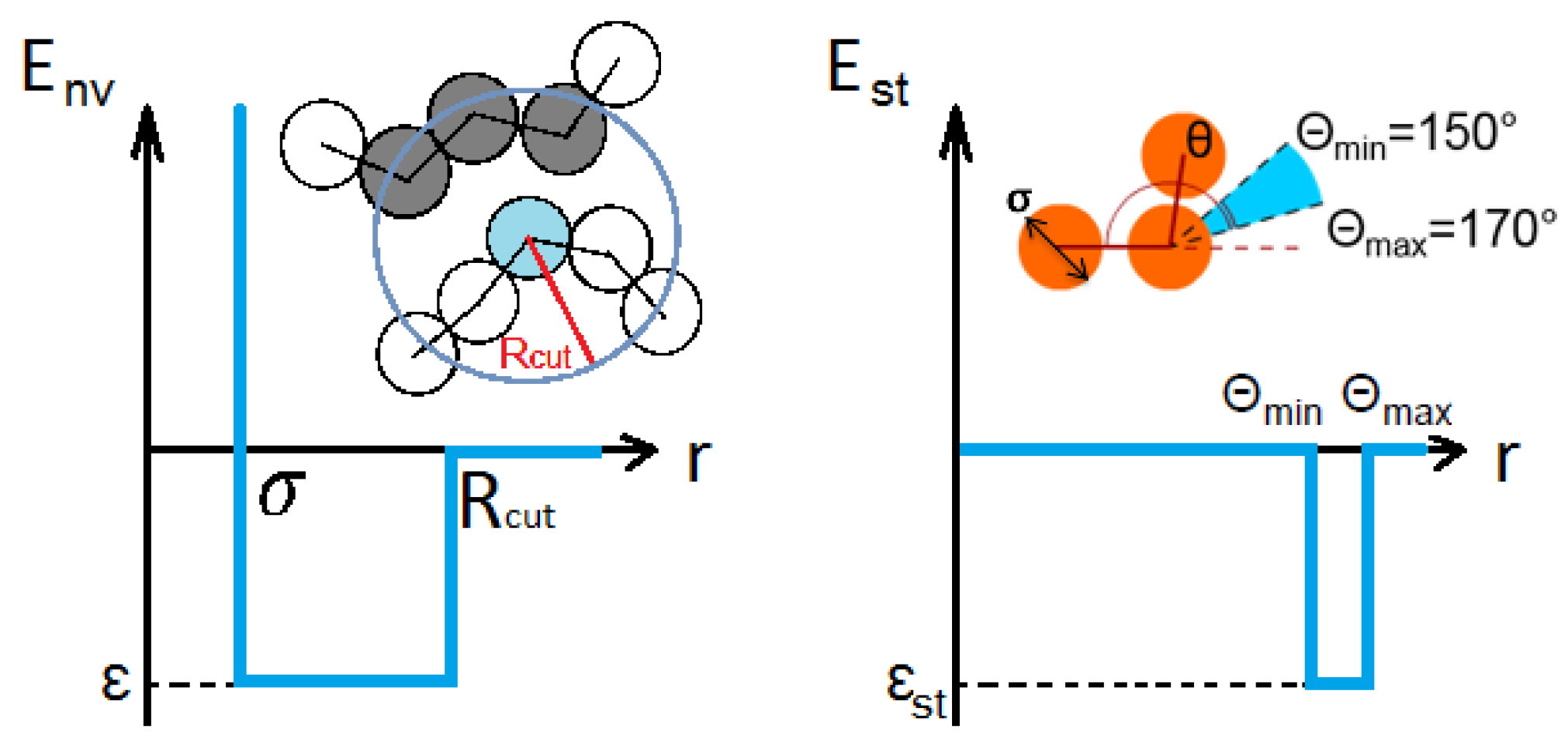
Abstract
1. Introduction
2. Model and Simulation Techniques
2.1. Model
2.2. SAMC Technique
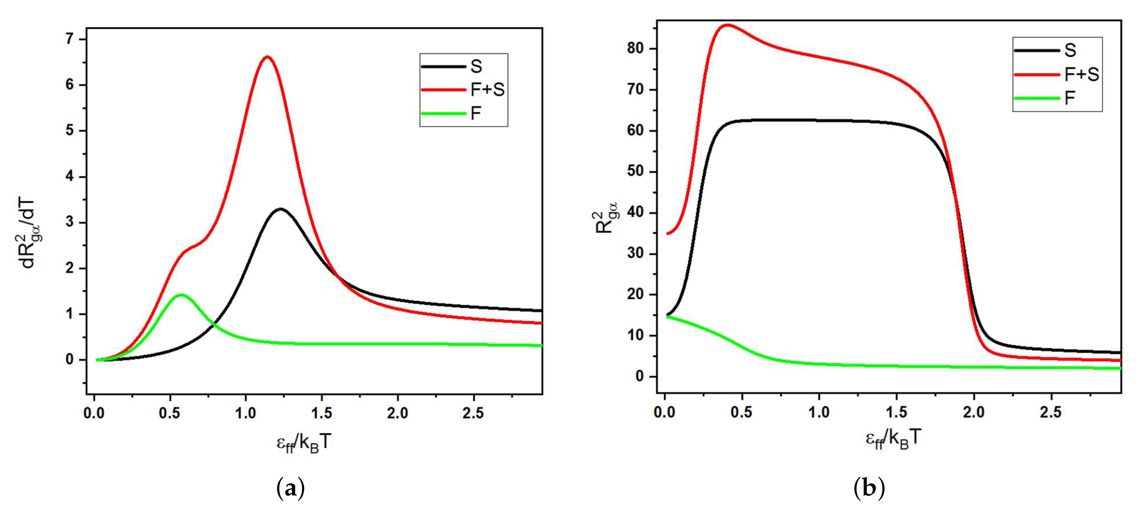
2.3. Canonical Analysis
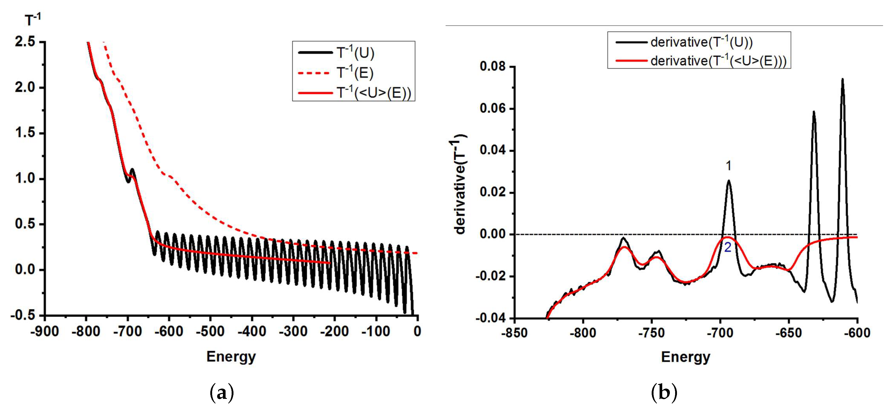
2.4. Microcanonical Analysis
3. Results and Discussion
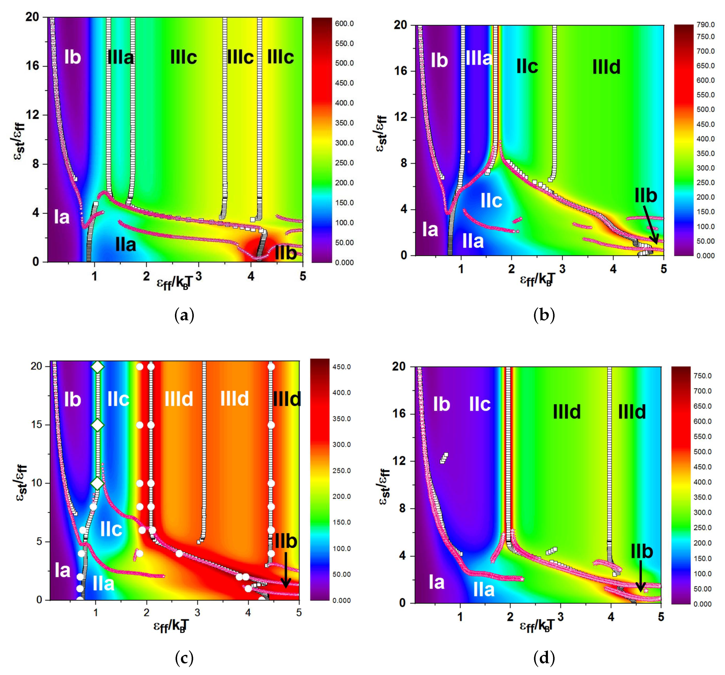
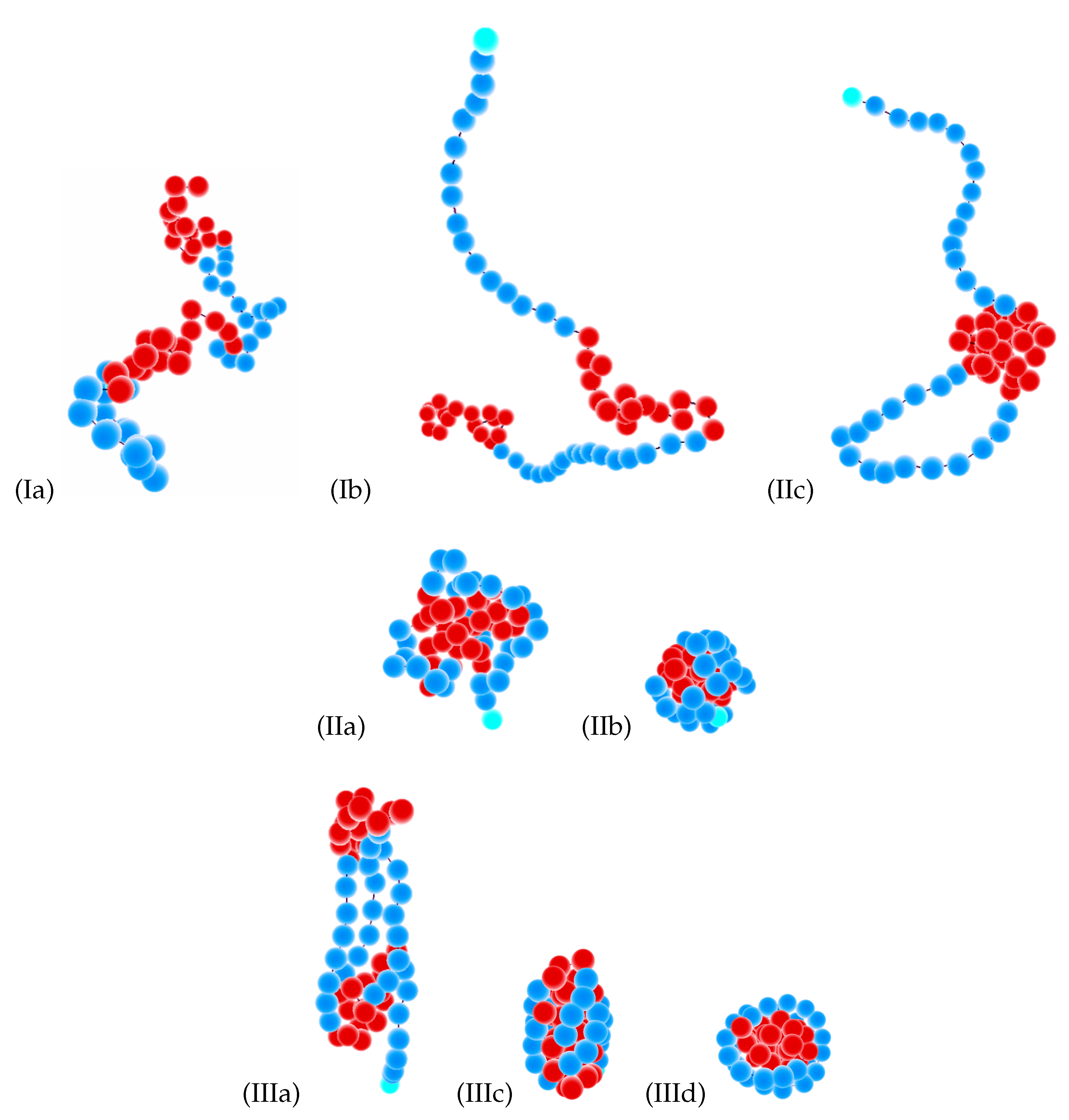
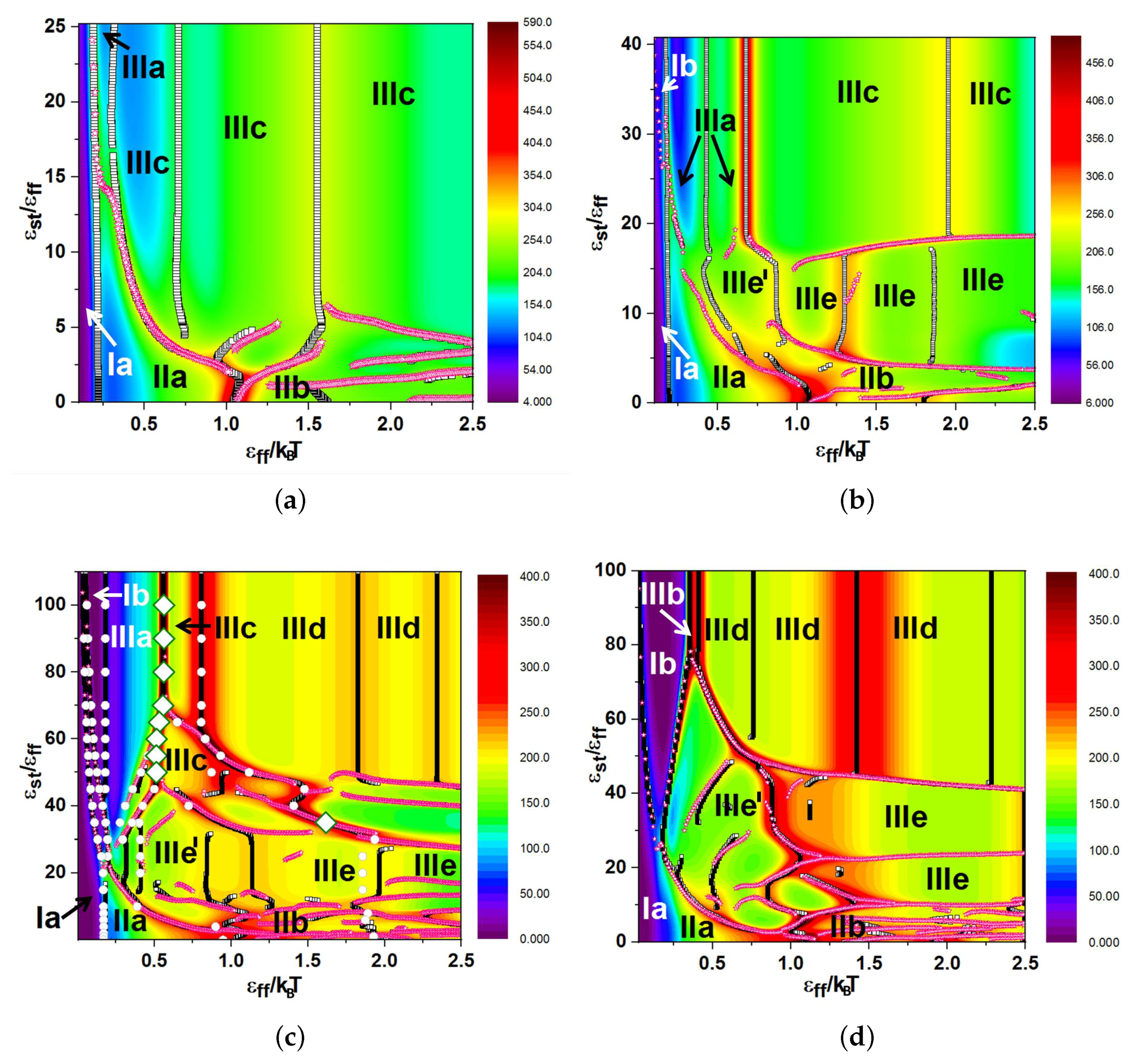
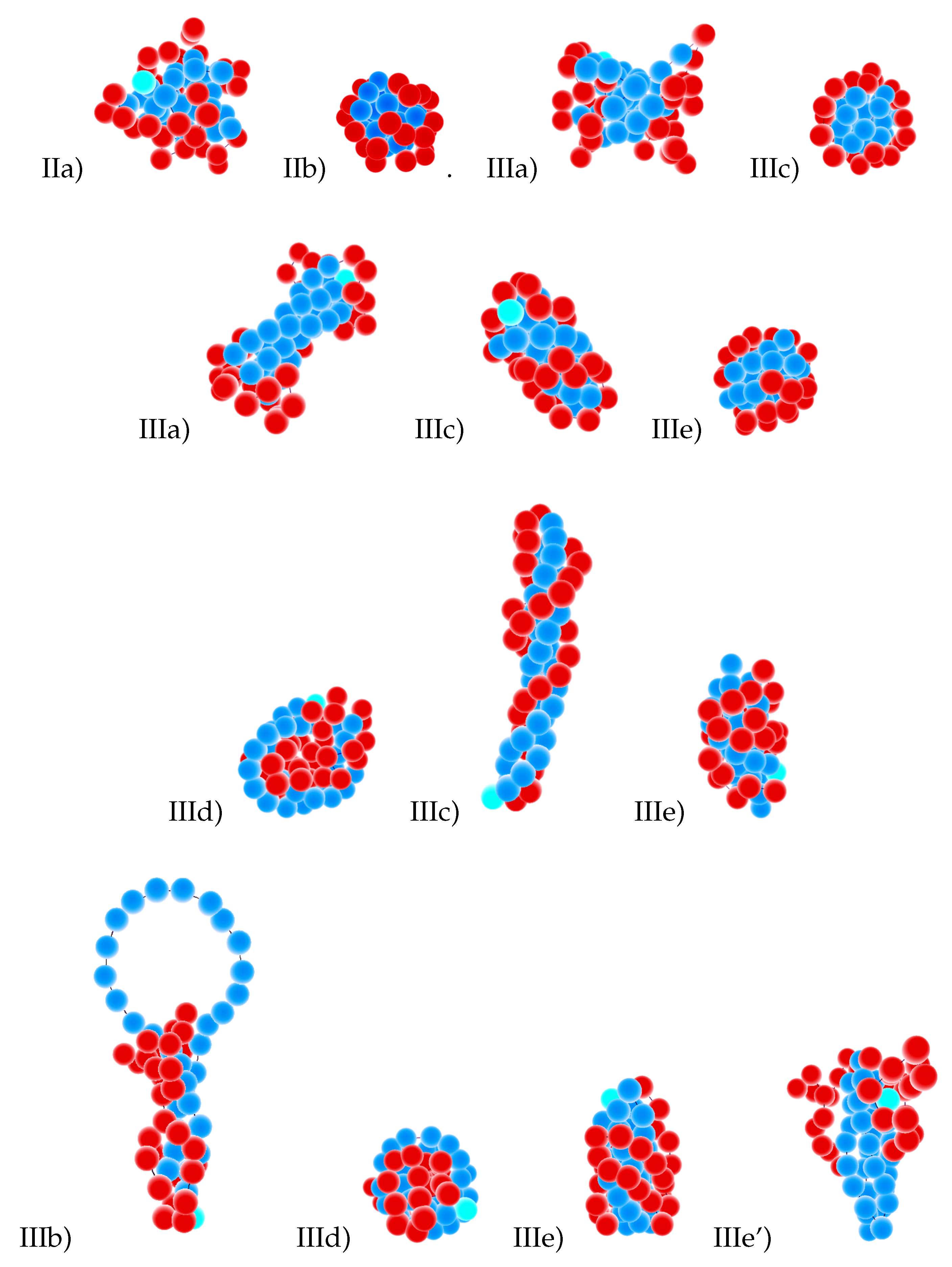
- The Roman number I stands for coils:
- (a)
- Ia = blocks of both types (F- and S-blocks) are coils;
- (b)
- Ib = F-blocks are coils, while S-blocks are extended.
- The Roman number II indicates isotropic globules:
- (a)
- IIa = liquid isotropic globule (F-core-S-shell or S-core-F-shell for the corresponding types of selective solvent);
- (b)
- IIb = frozen (solid) isotropic globule (F-core-S-shell or S-core-F-shell for the corresponding types of selective solvent);
- (c)
- IIc = “flower-like” globules and “tadpoles”, where only the flexible blocks are collapsed and aggregated into a single globule, while the semiflexible blocks form loops or tails.
- The Roman number III designates anisotropic globules:
- (a)
- IIIa = dumbbell globules, i.e., bundles of S-blocks forming a cylinder-like core (resembling a handle) with “caps” of F-beads at both ends of this handle;
- (b)
- IIIb = “tennis rackets”, i.e., globules where the S-blocks form this structure, while the F-monomers aggregate onto the shape defined by the S-blocks
- (c)
- IIIc = lamellar globules with the shape of prolate ellipsoids and with nematic ordering of S-blocks, but without folds inside S-blocks;
- (d)
- IIId = Saturn-like globules with an F-core and a toroidal S-shell;
- (e)
- IIIe = lamellar-like globules of the S-core-F-shell type with nematic ordering of S-blocks (and maybe also with translational ordering in the case of frozen globules) and with different numbers of folds in the S-blocks (leading to different numbers of S-stems in the core).
- Ia–Ib = no pseudo-phase transition can occur because this is just an sign. extension of semiflexible blocks, but there can be a maximum in the temperature dependence of the heat capacity (see below);
- Ia–IIa = coil–globule transition (second-order-like pseudo-phase transition from a coil to a liquid isotropic globule);
- Ib–IIc = collapse and aggregation of several liquid isotropic globules of F-blocks, while the S-blocks still stay extended (we found that the collapse of F-beads was always accompanied by their aggregation and therefore was registered as a first-order-like pseudo-phase transition);
- IIa–IIb = liquid–solid globule transition (first-order-like pseudo-phase transition from a liquid to a frozen globule);
- I–III = transitions between coils and globules with orientational ordering of bonds are usually first-order-like pseudo-phase transitions because they are accompanied by the generation of LC order (e.g., the formation of toroidal structures or the formation of bundles of stems);
- II–III = transitions between isotropic and anisotropic globules are usually first-order-like due to some underlying LC transitions;
- III–III = transitions between anisotropic globules with different types of symmetry in bond ordering could be both first- or second-order-like depending on the nature of the underlying structural changes.
3.1. Diagrams of States for the Case “F-Attract-Stronger”
3.2. Diagrams of States for the Case “S-Attract-Stronger”
4. Conclusions
Author Contributions
Funding
Acknowledgments
Conflicts of Interest
References
- Muraoka, T.; Kinbara, K. Bioinspired multi-block molecules. Chem. Commun. 2016, 52, 2667–2678. [Google Scholar] [CrossRef] [PubMed][Green Version]
- Stupp, S.I.; LeBonheur, V.; Walker, K.; Li, L.S.; Huggins, K.E.; Keser, M.; Amstutz, A. Supramolecular Materials: Self-Organized Nanostructures. Science 1997, 276, 384–389. [Google Scholar] [CrossRef]
- Topham, P.D.; Parnell, A.J.; Hiorns, R.C. Block copolymer strategies for solar cell technology. J. Polym. Sci. Part B Polym. Phys. 2011, 49, 1131–1156. [Google Scholar] [CrossRef]
- Petsko, G.; Ringe, D. Protein Structure and Function; Primers in Biology; Oxford University Press: Oxford, UK; New York, NY, USA, 2008. [Google Scholar]
- Lee, E.; Kim, J.K.; Lee, M. Tubular Stacking of Water-Soluble Toroids Triggered by Guest Encapsulation. J. Am. Chem. Soc. 2009, 131, 18242–18243. [Google Scholar] [CrossRef]
- Bates, F.S.; Hillmyer, M.A.; Lodge, T.P.; Bates, C.M.; Delaney, K.T.; Fredrickson, G.H. Multiblock Polymers: Panacea or Pandora’s Box? Science 2012, 336, 434–440. [Google Scholar] [CrossRef]
- Lo Verso, F.; Pomposo, J.A.; Colmenero, J.; Moreno, A.J. Simulation guided design of globular single-chain nanoparticles by tuning the solvent quality. Soft Matter 2015, 11, 1369–1375. [Google Scholar] [CrossRef]
- Hanlon, A.M.; Lyon, C.K.; Berda, E.B. What Is Next in Single-Chain Nanoparticles? Macromolecules 2016, 49, 2–14. [Google Scholar] [CrossRef]
- Zablotskiy, S.V.; Martemyanova, J.A.; Ivanov, V.A.; Paul, W. Diagram of states and morphologies of flexible-semiflexible copolymer chains: A Monte Carlo simulation. J. Chem. Phys. 2016, 144, 244903. [Google Scholar] [CrossRef]
- Zablotskiy, S.V.; Ivanov, V.A.; Paul, W. Multidimensional stochastic approximation Monte Carlo. Phys. Rev. E 2016, 93, 063303. [Google Scholar] [CrossRef] [PubMed]
- Zablotskiy, S.V.; Martemyanova, J.A.; Ivanov, V.A.; Paul, W. Stochastic approximation Monte Carlo algorithm for calculation of diagram of states of a single flexible-semiflexible copolymer chain. Polym. Sci. Ser. A 2016, 58, 899–915. [Google Scholar] [CrossRef]
- Liang, F. A Theory on Flat Histogram Monte Carlo Algorithms. J. Stat. Phys. 2006, 122, 511–529. [Google Scholar] [CrossRef]
- Liang, F.; Liu, C.; Carroll, R.J. Stochastic Approximation in Monte Carlo Computation. J. Am. Stat. Assoc. 2007, 102, 305–320. [Google Scholar] [CrossRef]
- Liang, F. On the use of stochastic approximation Monte Carlo for Monte Carlo integration. Stat. Probab. Lett. 2009, 79, 581–587. [Google Scholar] [CrossRef]
- Wang, F.; Landau, D.P. Efficient, Multiple-Range Random Walk Algorithm to Calculate the Density of States. Phys. Rev. Lett. 2001, 86, 2050–2053. [Google Scholar] [CrossRef]
- Wang, F.; Landau, D. Determining the density of states for classical statistical models: A random walk algorithm to produce a flat histogram. Phys. Rev. E 2001, 64, 056101. [Google Scholar] [CrossRef]
- Janke, W.; Paul, W. Thermodynamics and structure of macromolecules from flat-histogram Monte Carlo simulations. Soft Matter 2016, 12, 642–657. [Google Scholar] [CrossRef]
- Zhou, Y.; Hall, C.K.; Karplus, M. First-Order Disorder-to-Order Transition in an Isolated Homopolymer Model. Phys. Rev. Lett. 1996, 77, 2822–2825. [Google Scholar] [CrossRef]
- Zhou, Y.; Karplus, M.; Wichert, J.M.; Hall, C.K. Equilibrium thermodynamics of homopolymers and clusters: Molecular dynamics and Monte Carlo simulations of systems with square-well interactions. J. Chem. Phys. 1997, 107, 10691–10708. [Google Scholar] [CrossRef]
- Wüst, T.; Landau, D.P. Versatile Approach to Access the Low Temperature Thermodynamics of Lattice Polymers and Proteins. Phys. Rev. Lett. 2009, 102, 178101. [Google Scholar] [CrossRef] [PubMed]
- Gross, D.H.E. Microcanonical Thermodynamics: Phase Transitions in “Small” Systems; Lecture Notes in Physics; World Scientific: Singapore, 2001; Volume 66. [Google Scholar]
- Junghans, C.; Bachmann, M.; Janke, W. Microcanonical Analyses of Peptide Aggregation Processes. Phys. Rev. Lett. 2006, 97, 218103. [Google Scholar] [CrossRef] [PubMed]
- Lustig, R. Microcanonical Monte Carlo simulation of thermodynamic properties. J. Chem. Phys. 1998, 109, 8816–8828. [Google Scholar] [CrossRef]
- Martin-Mayor, V. Microcanonical Approach to the Simulation of First-Order Phase Transitions. Phys. Rev. Lett. 2007, 98, 137207. [Google Scholar] [CrossRef]
- Schierz, P.; Zierenberg, J.; Janke, W. First-order phase transitions in the real microcanonical ensemble. Phys. Rev. E 2016, 94, 021301. [Google Scholar] [CrossRef]
- Labastie, P.; Whetten, R.L. Statistical thermodynamics of the cluster solid-liquid transition. Phys. Rev. Lett. 1990, 65, 1567–1570. [Google Scholar] [CrossRef]
- Junghans, C.; Bachmann, M.; Janke, W. Thermodynamics of peptide aggregation processes: An analysis from perspectives of three statistical ensembles. J. Chem. Phys. 2008, 128, 085103. [Google Scholar] [CrossRef]
- Hernandez-Rojas, J.; Gomez Llorente, J.M. Microcanonical versus Canonical Analysis of Protein Folding. Phys. Rev. Lett. 2008, 100, 258104. [Google Scholar] [CrossRef]
- Dunkel, J.; Hilbert, S. Phase transitions in small systems: Microcanonical vs. canonical ensembles. Phys. A Stat. Mech. Appl. 2006, 370, 390–406. [Google Scholar] [CrossRef]
- Hilbert, S.; Dunkel, J. Nonanalytic microscopic phase transitions and temperature oscillations in the microcanonical ensemble: An exactly solvable one-dimensional model for evaporation. Phys. Rev. E 2006, 74, 011120. [Google Scholar] [CrossRef]
- Taylor, M.P.; Paul, W.; Binder, K. Phase transitions of a single polymer chain: A Wang–Landau simulation study. J. Chem. Phys. 2009, 131, 114907. [Google Scholar] [CrossRef]
- Zierenberg, J.; Marenz, M.; Janke, W. Dilute Semiflexible Polymers with Attraction: Collapse, Folding and Aggregation. Polymers 2016, 8, 333. [Google Scholar] [CrossRef]
- Grosberg, A.Y.; Khokhlov, A.R. Statistical theory of polymeric lyotropic liquid crystals. Adv. Polym. Sci. 1981, 41, 53–97. [Google Scholar]
- Wang, Z.; Wang, L.; He, X. Phase transition of a single protein-like copolymer chain. Soft Matter 2013, 9, 3106–3116. [Google Scholar] [CrossRef]
- Wang, W.; Zhao, P.; Yang, X.; Lu, Z.Y. Coil-to-globule transitions of homopolymers and multiblock copolymers. J. Chem. Phys. 2014, 141, 244907. [Google Scholar] [CrossRef] [PubMed]
- Cooke, I.R.; Williams, D.R.M. Collapse of Flexible-Semiflexible Copolymers in Selective Solvents: Single Chain Rods, Cages, and Networks. Macromolecules 2004, 37, 5778–5783. [Google Scholar] [CrossRef]
- Parsons, D.F.; Williams, D.R.M. Single Chains of Block Copolymers in Poor Solvents: Handshake, Spiral, and Lamellar Globules Formed by Geometric Frustration. Phys. Rev. Lett. 2007, 99, 228302. [Google Scholar] [CrossRef]
- Fytas, N.G.; Theodorakis, P.E. Analysis of the static properties of cluster formations in symmetric linear multiblock copolymers. J. Phys. Condens. Matter 2011, 23, 235106. [Google Scholar] [CrossRef] [PubMed]
- Rissanou, A.N.; Tzeli, D.S.; Anastasiadis, S.H.; Bitsanis, I.A. Collapse transitions in thermosensitive multi-block copolymers: A Monte Carlo study. J. Chem. Phys. 2014, 140, 204904. [Google Scholar] [CrossRef]
- Woloszczuk, S.; Banaszak, M.; Knychala, P.; Lewandowski, K.; Radosz, M. Alternating multiblock copolymers exhibiting protein-like transitions in selective solvents: A Monte Carlo study. J. Non-Cryst. Solids 2008, 354, 4138–4142. [Google Scholar] [CrossRef]
- Lewandowski, K.; Knychala, P.; Banaszak, M. Protein-like behavior of multiblock copolymer chains in a selective solvent by a variety of lattice and off-lattice Monte Carlo simulations. Phys. Status Solidi (b) 2008, 245, 2524–2532. [Google Scholar] [CrossRef]
- Nowak, C.; Rostiashvili, V.G.; Vilgis, T.A. Globular structures of a helix-coil copolymer: Self-consistent treatment. J. Chem. Phys. 2007, 126, 034902. [Google Scholar] [CrossRef]
- Seaton, D.T.; Schnabel, S.; Landau, D.P.; Bachmann, M. From Flexible to Stiff: Systematic Analysis of Structural Phases for Single Semiflexible Polymers. Phys. Rev. Lett. 2013, 110, 028103. [Google Scholar] [CrossRef]
- Marenz, M.; Janke, W. Knots as a Topological Order Parameter for Semiflexible Polymers. Phys. Rev. Lett. 2016, 116, 128301. [Google Scholar] [CrossRef]
- Shakirov, T.; Zablotskiy, S.; Böker, A.; Ivanov, V.; Paul, W. Comparison of Boltzmann and Gibbs entropies for the analysis of single-chain phase transitions. Eur. Phys. J. Spec. Top. 2017, 226, 705–723. [Google Scholar] [CrossRef]
- Sethna, J.P. Statistical Mechanics: Entropy, Order Parameters and Complexity; Oxford Master Series in Physics; Oxford University Press: Oxford, UK, 2006. [Google Scholar]
- Werlich, B.; Taylor, M.; Shakirov, T.; Paul, W. On the Pseudo Phase Diagram of Single Semi-Flexible Polymer Chains: A Flat-Histogram Monte Carlo Study. Polymers 2017, 9, 38. [Google Scholar] [CrossRef]
- Schnabel, S.; Seaton, D.T.; Landau, D.P.; Bachmann, M. Microcanonical entropy inflection points: Key to systematic understanding of transitions in finite systems. Phys. Rev. E 2011, 84, 011127. [Google Scholar] [CrossRef] [PubMed]
- Rocha, J.C.S.; Schnabel, S.; Landau, D.P.; Bachmann, M. Identifying transitions in finite systems by means of partition function zeros and microcanonical inflection-point analysis: A comparison for elastic flexible polymers. Phys. Rev. E 2014, 90, 022601. [Google Scholar] [CrossRef]
- Schierz, P.; Zierenberg, J.; Janke, W. Molecular Dynamics and Monte Carlo simulations in the microcanonical ensemble: Quantitative comparison and reweighting techniques. J. Chem. Phys. 2015, 143, 134114. [Google Scholar] [CrossRef]
- Zierenberg, J.; Schierz, P.; Janke, W. Canonical free-energy barrier of particle and polymer cluster formation. Nat. Commun. 2017, 8, 14546. [Google Scholar] [CrossRef] [PubMed]
- Janke, W.; Schierz, P.; Zierenberg, J. Transition barrier at a first-order phase transition in the canonical and microcanonical ensemble. J. Phys. Conf. Ser. 2017, 921, 012018. [Google Scholar] [CrossRef]
- Sommerfeld, A. Vorlesungen über Theoretische Physik (Band 5): Thermodynamik und Statistik; Verlag Harri Deutsch: Frankfurt am Main, Germany, 2011. [Google Scholar]
- Paul, W.; Müller, M. Enhanced sampling in simulations of dense systems: The phase behavior of collapsed polymer globules. J. Chem. Phys. 2001, 115, 630–635. [Google Scholar] [CrossRef]
- Martemyanova, J.A.; Stukan, M.R.; Ivanov, V.A.; Müller, M.; Paul, W.; Binder, K. Dense orientationally ordered states of a single semiflexible macromolecule: An expanded ensemble Monte Carlo simulation. J. Chem. Phys. 2005, 122, 174907. [Google Scholar] [CrossRef]
- Ivanov, V.A.; Stukan, M.R.; Vasilevskaya, V.V.; Paul, W.; Binder, K. Structures of stiff macromolecules of finite chain length near the coil-globule transition: A Monte Carlo simulation. Macromol. Theory Simul. 2000, 9, 488–499. [Google Scholar] [CrossRef]
- Ivanov, V.A.; Paul, W.; Binder, K. Finite chain length effects on the coil-globule transition of stiff-chain macromolecules: A Monte Carlo simulation. J. Chem. Phys. 1998, 109, 5659–5669. [Google Scholar] [CrossRef]
- Stukan, M.R.; Ivanov, V.A.; Grosberg, A.Y.; Paul, W.; Binder, K. Chain length dependence of the state diagram of a single stiff-chain macromolecule: Theory and Monte Carlo simulation. J. Chem. Phys. 2003, 118, 3392–3400. [Google Scholar] [CrossRef]
- Blundell, S. Magnetism In Condensed Matter; Oxford Master Series in Physics; Oxford University Press: Oxford, UK, 2000. [Google Scholar]
- Gopal, E. Specific Heats at Low Temperatures; Springer US: New York, NY, USA: 1966; Volume 66. [Google Scholar]
- Binder, K. Finite size effects at phase transitions. In Computational Methods in Field Theory; Lecture Notes in Physics; Gausterer, H., Lang, C.B., Eds.; Springer: Berlin/Heidelberg, Germany, 1992; pp. 59–125. [Google Scholar]
- Sadovnichy, V.; Tikhonravov, A.; Voevodin, V.; Opanasenko, V. “Lomonosov”: Supercomputing at Moscow State University. In Contemporary High Performance Computing: From Petascale toward Exascale; Vetter, J.S., Ed.; Chapman & Hall/CRC Computational Science Series; CRC Press: Boca Raton, FL, USA, 2013; pp. 283–307. [Google Scholar]


© 2019 by the authors. Licensee MDPI, Basel, Switzerland. This article is an open access article distributed under the terms and conditions of the Creative Commons Attribution (CC BY) license (http://creativecommons.org/licenses/by/4.0/).
Share and Cite
Maltseva, D.; Zablotskiy, S.; Martemyanova, J.; Ivanov, V.; Shakirov, T.; Paul, W. Diagrams of States of Single Flexible-Semiflexible Multi-Block Copolymer Chains: A Flat-Histogram Monte Carlo Study. Polymers 2019, 11, 757. https://doi.org/10.3390/polym11050757
Maltseva D, Zablotskiy S, Martemyanova J, Ivanov V, Shakirov T, Paul W. Diagrams of States of Single Flexible-Semiflexible Multi-Block Copolymer Chains: A Flat-Histogram Monte Carlo Study. Polymers. 2019; 11(5):757. https://doi.org/10.3390/polym11050757
Chicago/Turabian StyleMaltseva, Daria, Sergey Zablotskiy, Julia Martemyanova, Viktor Ivanov, Timur Shakirov, and Wolfgang Paul. 2019. "Diagrams of States of Single Flexible-Semiflexible Multi-Block Copolymer Chains: A Flat-Histogram Monte Carlo Study" Polymers 11, no. 5: 757. https://doi.org/10.3390/polym11050757
APA StyleMaltseva, D., Zablotskiy, S., Martemyanova, J., Ivanov, V., Shakirov, T., & Paul, W. (2019). Diagrams of States of Single Flexible-Semiflexible Multi-Block Copolymer Chains: A Flat-Histogram Monte Carlo Study. Polymers, 11(5), 757. https://doi.org/10.3390/polym11050757