Mathematical Modeling and Simulations for Large-Strain J-Shaped Diagrams of Soft Biological Materials


Abstract
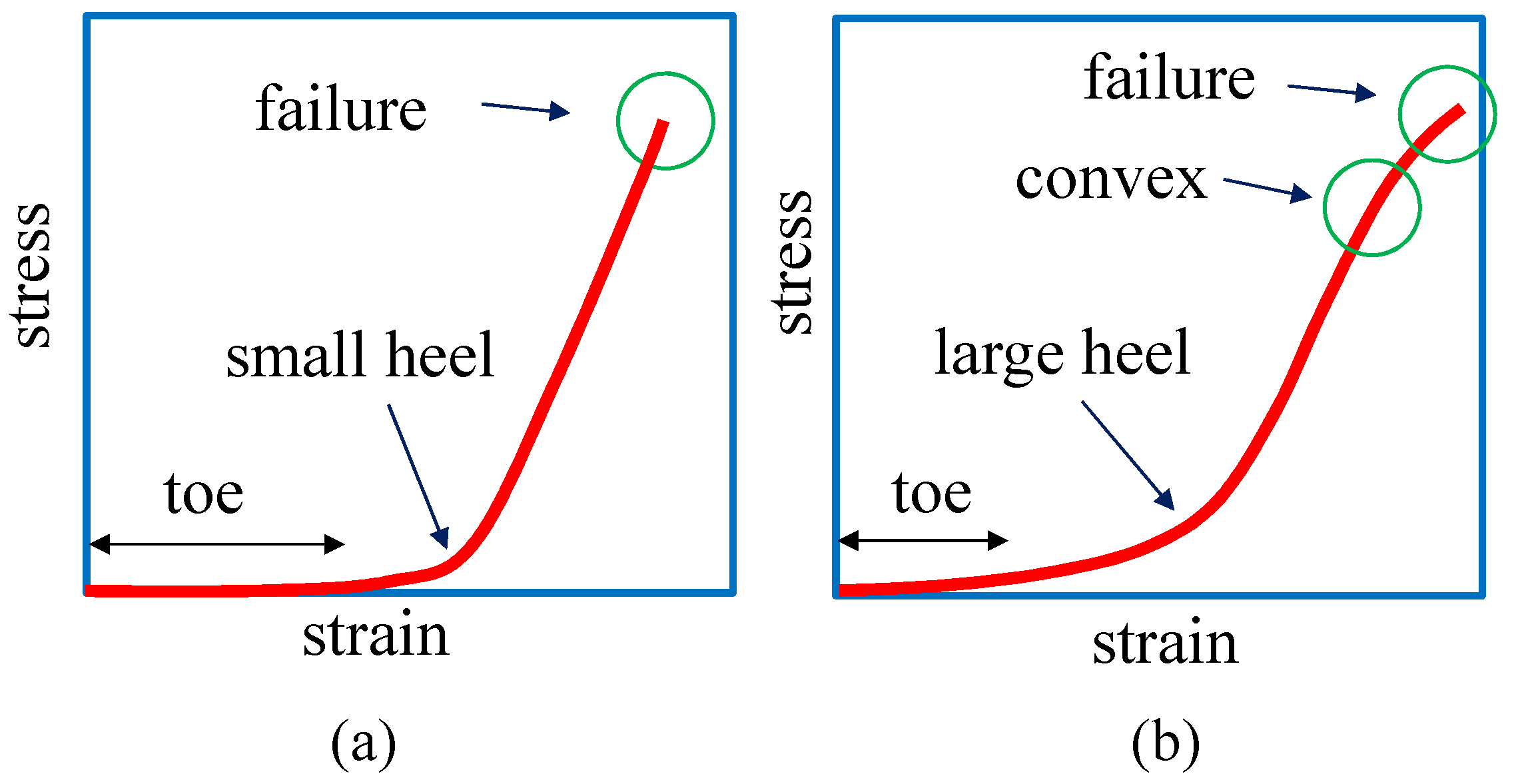
1. Introduction
2. Models and Monte Carlo Simulations
2.1. 2D Model
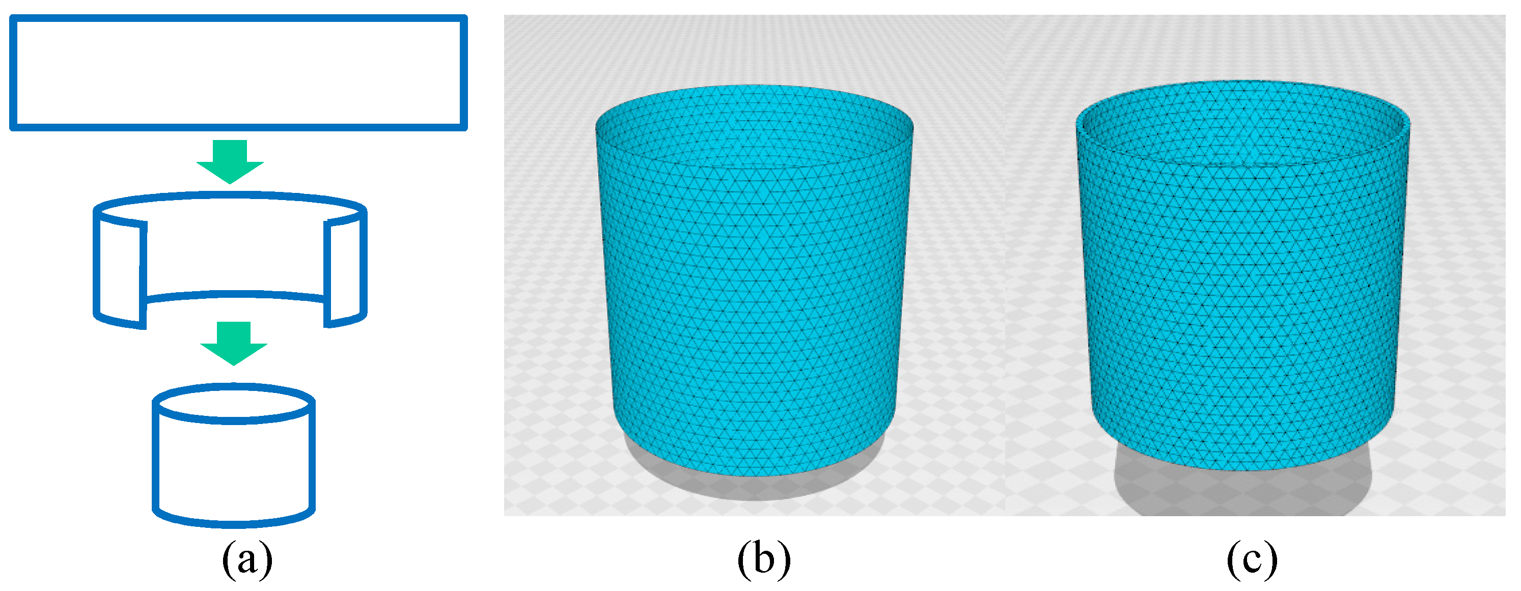
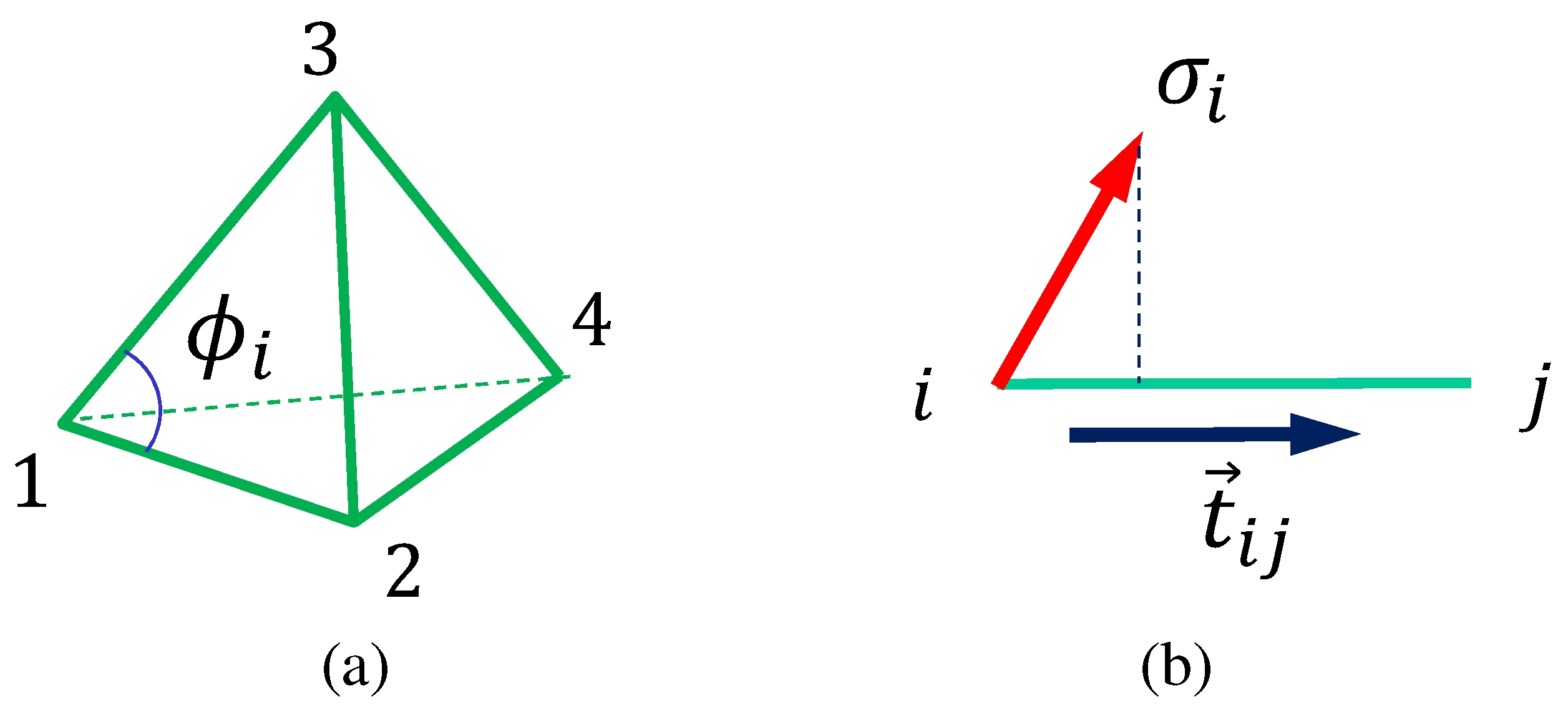
2.2. 3D Model
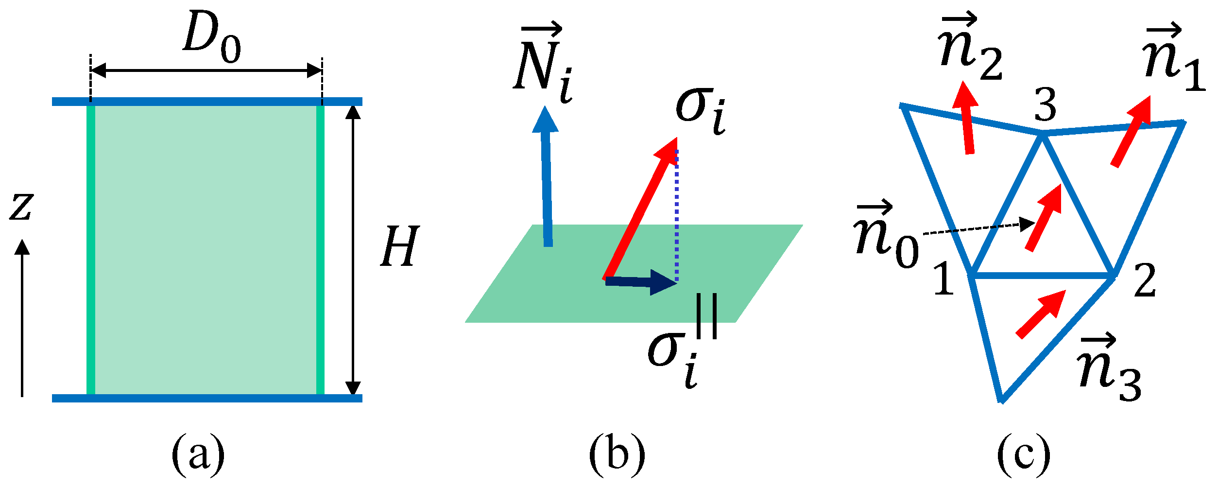
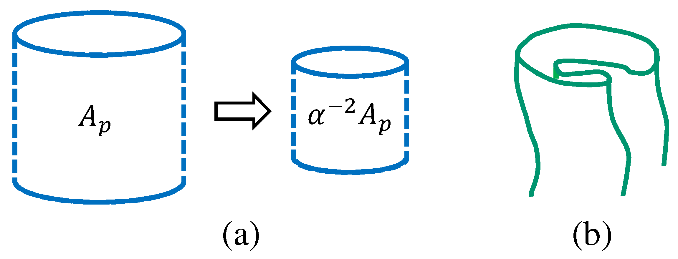
2.3. Formula for Stress Calculation
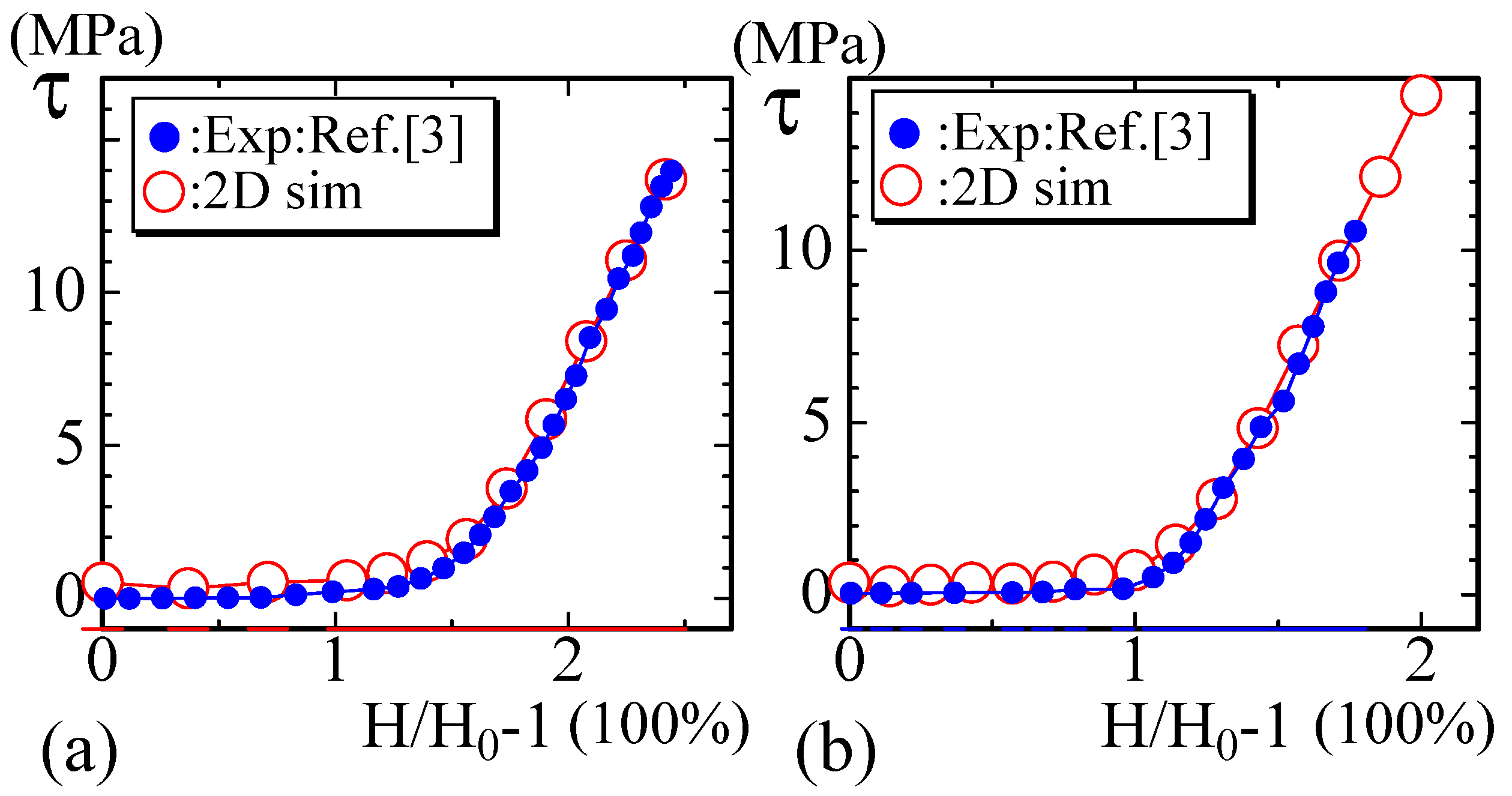
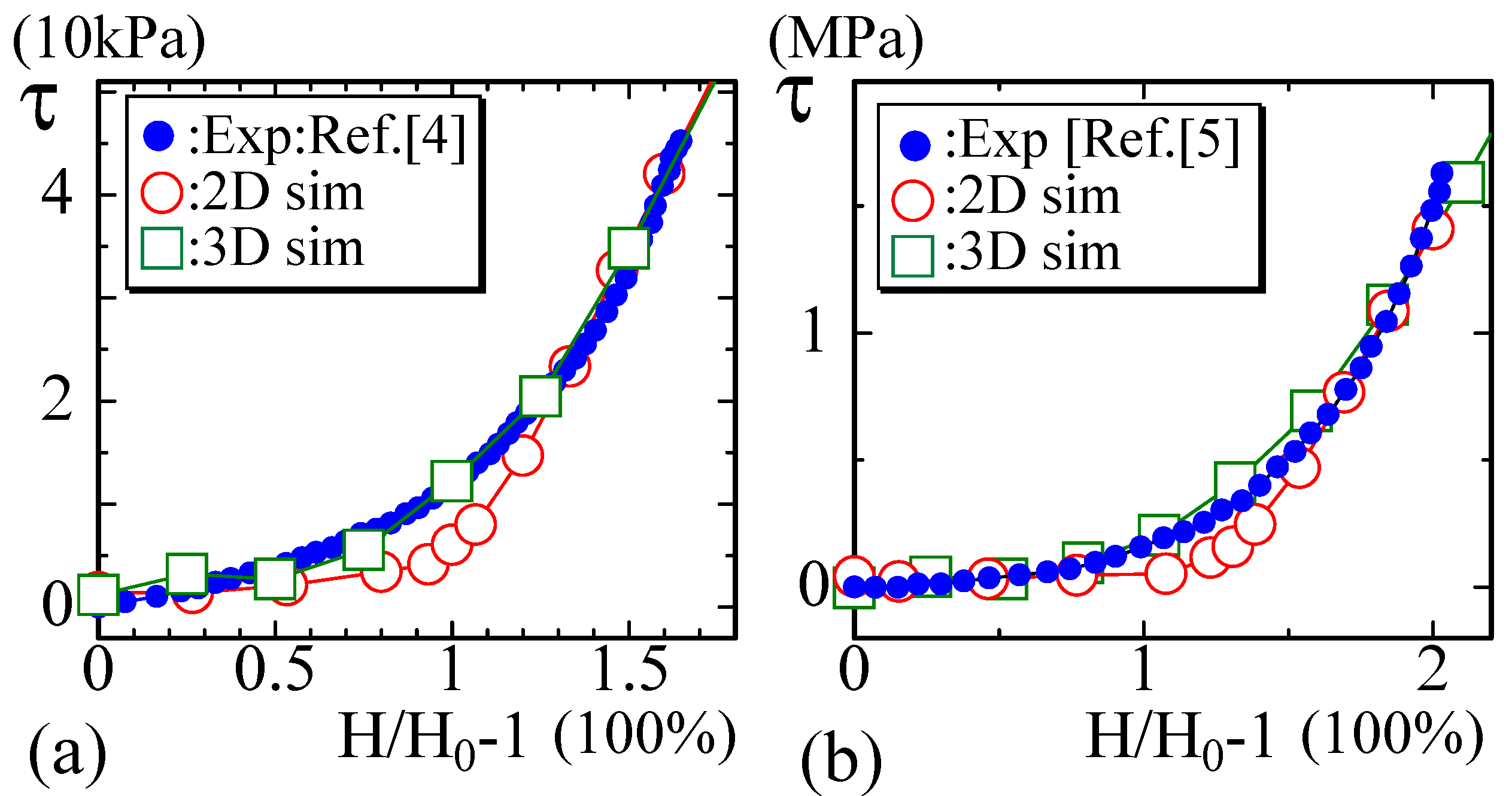
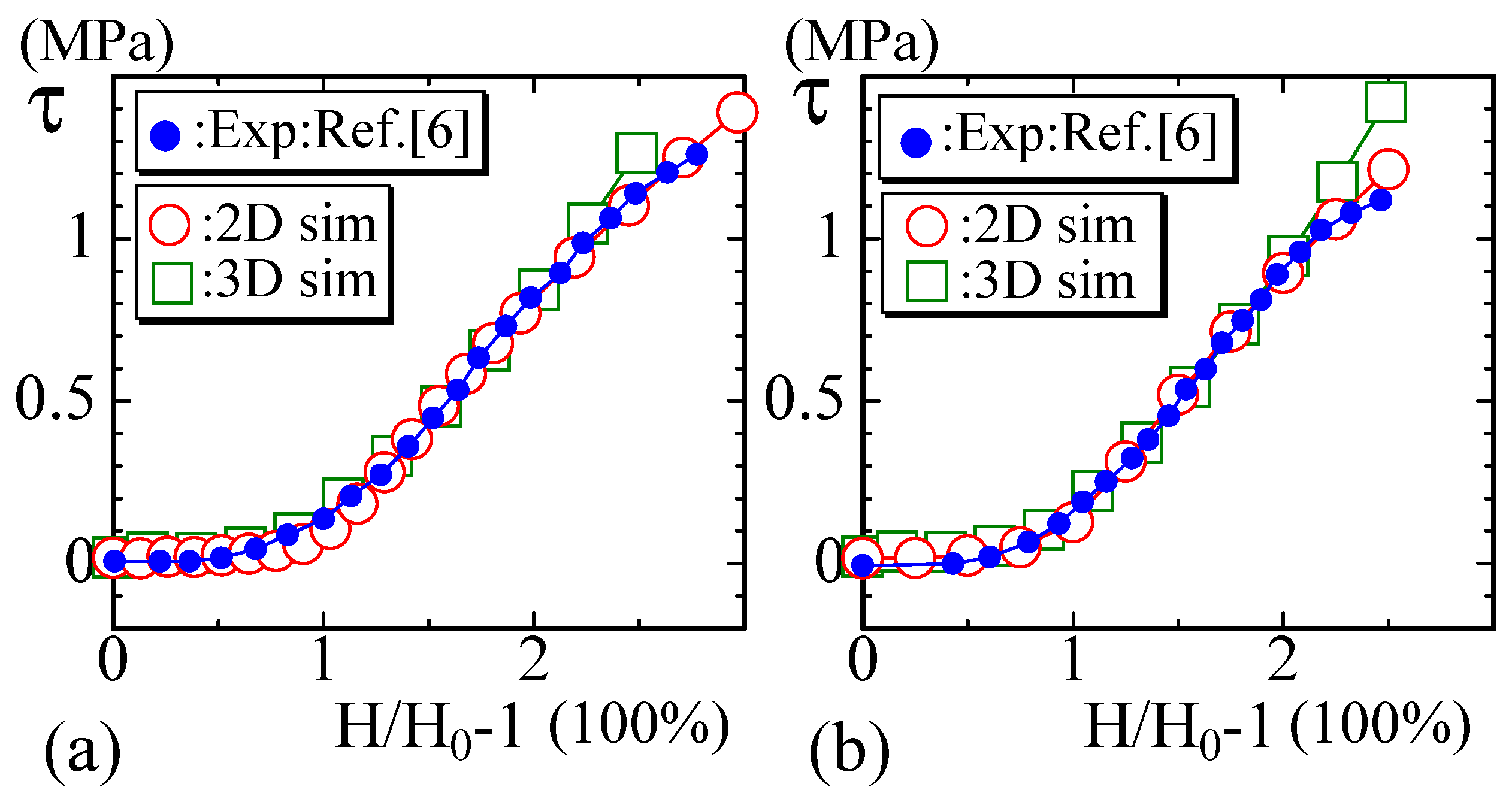
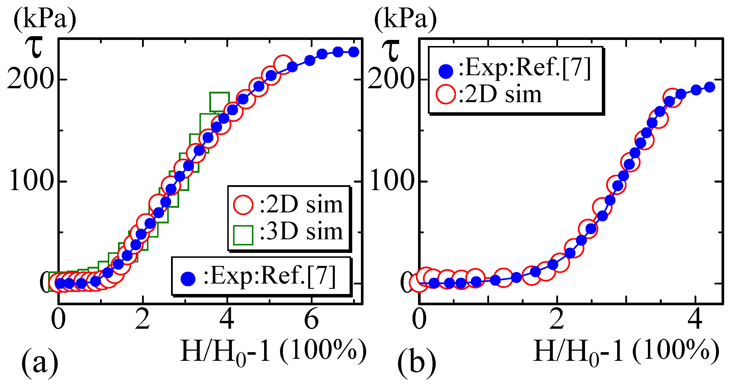
2.4. Comparison with Experimental Data
2.5. Monte Carlo Technique
3. Simulation Results
3.1. Comparison with Experimental Data
3.2. Dependence of the Results on the Simulation Parameters
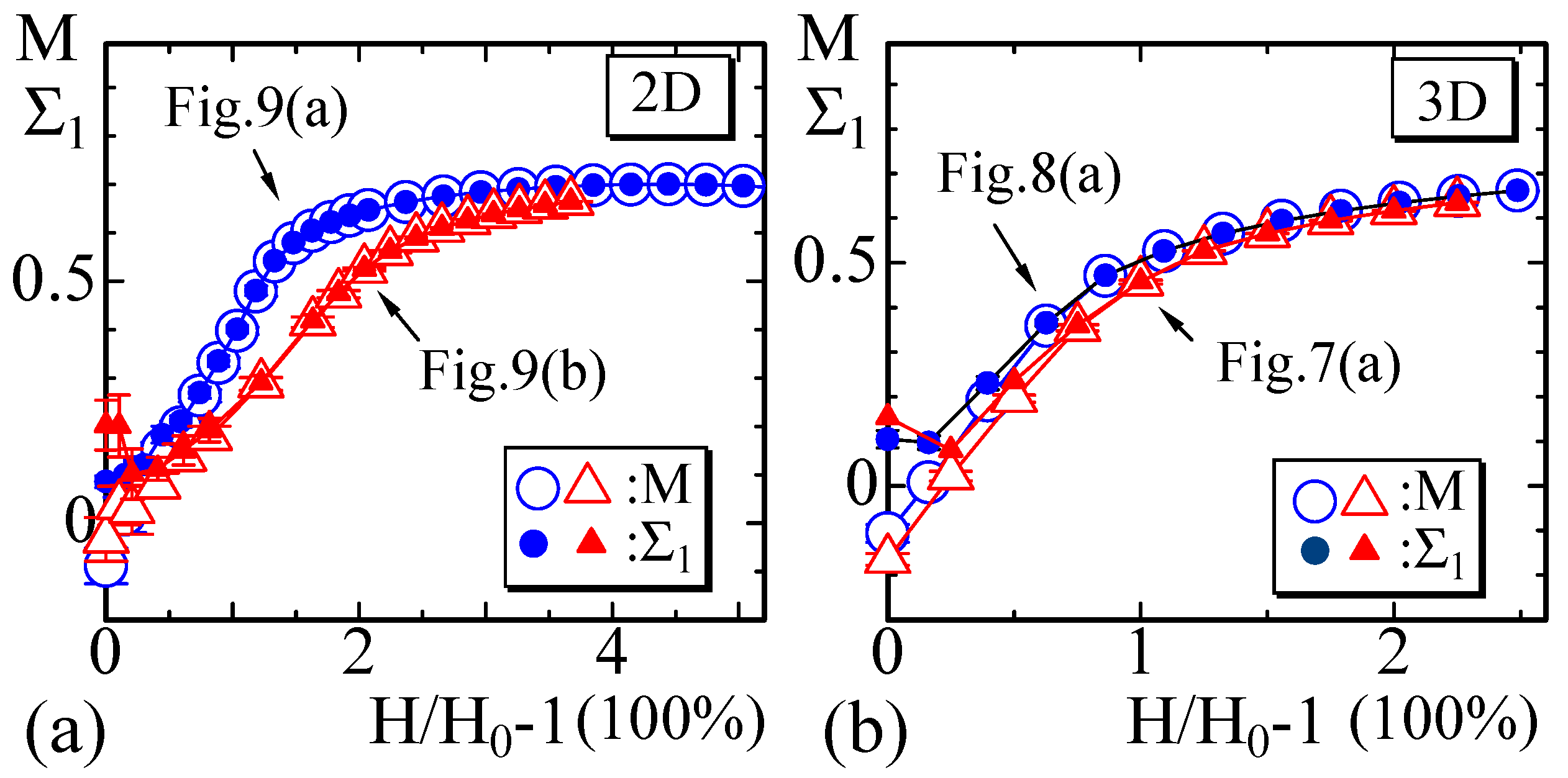
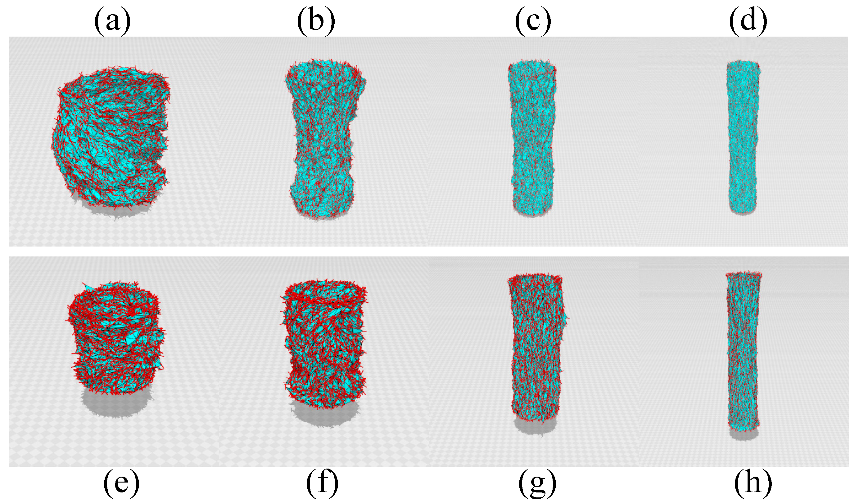
3.3. Behavior of the Variable and Snapshots
4. Summary and Conclusions
4.1. On the FG Modeling
4.2. Concluding Remarks
Author Contributions
Funding
Acknowledgments
Conflicts of Interest
Abbreviations
| 2D | 2-dimensional |
| 3D | 3-dimensional |
| S-heel | small heel |
| L-heel | large heel |
| FG | Finsler geometry |
| MC | Monte Carlo |
References
- Meyers, M.A.; Chen, P.; Lin, A.Y.; Seki, Y. Biological materials: Structure and mechanical properties. Prog. Mater. Sci. 2008, 53, 1–206. [Google Scholar] [CrossRef]
- Gautieri, A.; Vesentini, S.; Redaelli, A.; Buehler, M.J. Hierarchical Structure and Nanomechanics of Collagen Microfibrils from the Atomistic Scale Up. Nano Lett. 2011, 11, 757–766. [Google Scholar] [CrossRef] [PubMed]
- Xiong, Y.; Duong, P.L.T.; Raghavan, N.; Rosen, D.W. A rapid design exploration framework under additive manufacturing process uncertainty. In Proceedings of the 3rd International Conference on Progress in Additive Manufacturing (Pro-AM 2018), Singapore, 14–17 May 2018. [Google Scholar]
- Jang, K.-I.; Chung, H.U.; Xu, S.; Lee, C.H.; Luan, H.; Jeong, J.; Cheng, H.; Kim, G.-T.; Han, S.Y.; Lee, J.W.; et al. Soft network composite materials with deterministic and bio-inspired designs. Nat. Commun. 2015, 6, 6566. [Google Scholar] [CrossRef] [PubMed]
- Rivera, G.; Savitzky, A.H.; Hinkley, J.A. Mechanical properties of the integument of the common gartersnake, Thamnophis sirtalis (Serpentes: Colubridae). J. Exp. Biol. 2005, 208, 2913–2922. [Google Scholar] [CrossRef] [PubMed]
- Lopez, M.A.; Pardo, P.S.; Cox, G.A.; Boriek, A.M. Early mechanical dysfunction of the diaphragm in the muscular dystrophy with myositis (Ttnmdm) model. Am. J. Physiol. Cell Physiol. 2008, 295, C1092–C1102. [Google Scholar] [CrossRef] [PubMed]
- Arroyave, G.A.I.; Lima, R.G.; Martins, P.A.L.S.; Ramiäo, N.; Jorge, R.M.N. Methodology for Mechanical Characterization of Soft Biological Tissues: Arteries. Procedia Eng. 2015, 110, 74–81. [Google Scholar]
- Komatsu, K.; Kanazashi, M.; Shimada, A.; Shibata, T.; Viidik, A.; Chiba, M. Effects of age on the stress–strain and stress-relaxation properties of the rat molar periodontal ligament. Arch. Oral Biol. 2004, 49, 817–824. [Google Scholar] [CrossRef] [PubMed]
- Granzier, H.L.; Irving, T.C. Passive Tension in Cardiac Muscle: Contribution of Collagen, Titin, Microtubules, and Intermediate Filaments. Biophys. J. 1995, 68, 1027–1044. [Google Scholar] [CrossRef]
- Dunn, M.G.; Silver, F.H.; Swan, D.A. Mechanical Analysis of Hypertrophic Scar Tissue: Structural Basis for Apparent Increased Rigidity. J. Investig. Dermatol. 1985, 84, 9–13. [Google Scholar] [CrossRef]
- Frederick, H.S.; Joseph, W.F.; Dale, D. Viscoelastic Properties of Human Skin and Processed Demis. Skin Res. Technol. 2001, 7, 18–23. [Google Scholar]
- Spencer, P.L.; Kristin, S.M.; Dawn, M.E.; Louis, J.S. Effect of Fiber Distribution and Realignment on the Nonlinear and Inhomogeneous Mechanical Properties of Human Supraspinatus Tendon under Longitudinal Tensile Loading. J. Orthop. Res. 2009, 12, 1596–1602. [Google Scholar]
- Fratzl, P.; Misof, K.; Zizak, I.; Rapp, G.; Amenitsch, H.; Bernstorff, S. Fibrillar Structure and Mechanical Properties of Collagen. J. Struct. Biol. 1997, 122, 119–122. [Google Scholar] [CrossRef] [PubMed]
- Chowa, J.P.; Simionescu, D.T.; Warner, H.; Wang, B.; Patnaik, S.S.; Liao, J.; Simionescu, A. Mitigation of diabetes-related complications in implanted collagen and elastin scaffolds using matrix-binding polyphenol. Biomaterials 2013, 34, 685–695. [Google Scholar] [CrossRef] [PubMed]
- Greven, H.; Zanger, K.; Schwinger, G. Mechanical Properties of the Skin of Xenopus laevis (Anura, Amphibia). J. Morphol. 1995, 224, 15–22. [Google Scholar] [CrossRef] [PubMed]
- Tronci, G.; Doyle, A.; Russell, S.J.; Wood, D.J. Triple-helical collagen hydrogels via covalent aromatic functionalisation with 1,3-phenylenediacetic acid. J. Mater. Chem. B 2013, 1, 5478–5488. [Google Scholar] [CrossRef] [PubMed]
- Toscano, A.E.; Ferraz, K.M.; de Castro, R.M.; Canon, F. Passive stiffness of rat skeletal muscle undernourished during fetal development. Clinics 2010, 65, 1363–1369. [Google Scholar] [CrossRef] [PubMed]
- Roeder, B.A.; Kokini, K.; Sturgis, J.E.; Robinson, J.P.; Voytik-Harbin, S.L. Tensile Mechanical Properties of Three-Dimensional Type I Collagen Extracellular Matrices With Varied Microstructure. J. Biomed. Eng. Trans. ASME 2002, 124, 214–222. [Google Scholar] [CrossRef]
- Seliktar, D.; Black, R.A.; Vito, R.P.; Nerem, R.M. Dynamic Mechanical Conditioning of Collagen-Gel Blood Vessel Constructs Induces Remodeling In Vitro. Ann. Biomed. Eng. 2000, 28, 351–362. [Google Scholar] [CrossRef] [PubMed]
- Warner, M.; Terentjev, E.M. Liquid Crystal Elastomer; Oxford University Press: Oxford, UK, 2003. [Google Scholar]
- Domenici, V. 2H NMR studies of liquid crystal elastomers: Macroscopic vs. molecular properties. Prog. Nucl. Mag. Reson. Spectrosc. 2012, 63, 1–32. [Google Scholar] [CrossRef] [PubMed]
- Lubensky, T.C.; Mukhopadhyay, R.; Radzihovsky, L.; Xing, X. Symmetries and elasticity of nematic gels. Phys. Rev. E 2002, 66, 011702. [Google Scholar] [CrossRef] [PubMed]
- Xing, X.; Mukhopadhyay, R.; Lubensky, T.C.; Radzihovsky, L. Fluctuating nematic elastomer membranes. Phys. Rev. E 2003, 68, 021108. [Google Scholar] [CrossRef] [PubMed]
- Xing, X.; Radzihovsky, L. Nonlinear elasticity, fluctuations and heterogeneity of nematic elastomers. Ann. Phys. 2008, 323, 105–203. [Google Scholar] [CrossRef]
- Stenull, O.; Lubensky, T.C. Phase Transitions and Soft Elasticity of Smectic Elastomers. Phys. Rev. Lett. 2005, 94, 018304. [Google Scholar] [CrossRef] [PubMed]
- Stenull, O.; Lubensky, T.C. Soft elasticity in biaxial smectic and smectic-C elastomers. Phys. Rev. E 2006, 74, 051709. [Google Scholar] [CrossRef] [PubMed]
- Ogden, R.W. Non-Linear Elastic Deformations, 2nd ed.; Dover: New York, NY, USA, 1997. [Google Scholar]
- Fung, Y.C. Biomechanics: Mechanical Properties of Living Tissues, 2nd ed.; Springer: New York, NY, USA, 1993. [Google Scholar]
- Temmen, H.; Pleiner, H.; Liu, M.; Brand, H.R. Convective Nonlinearity in Non-Newtonian Fluids. Phys. Rev. Lett. 2000, 84, 3228–3231. [Google Scholar] [CrossRef] [PubMed]
- Pleiner, H.; Liu, M.; Brand, H.R. The structure of convective nonlinearities in polymer rheology. Rheol. Acta 2000, 39, 560–565. [Google Scholar] [CrossRef]
- Koibuchi, H.; Sekino, H. Monte Carlo studies of a Finsler geometric surface model. Physics A 2014, 393, 37–50. [Google Scholar] [CrossRef]
- Osari, K.; Koibuchi, H. Finsler geometry modeling and Monte Carlo study of 3D liquid crystal elastomer. Polymer 2017, 114, 355. [Google Scholar] [CrossRef]
- Takano, Y.; Koibuchi, H. J-shaped stress–strain diagram of collagen fibers: Frame tension of triangulated surfaces with fixed boundaries. Phys. Rev. E 2017, 95, 042411. [Google Scholar] [CrossRef] [PubMed]
- Takano, Y.; Koibuchi, H. Finsler geometry modeling for J-shaped stress–strain diagram of collagen fiber networks. Proc. Mater. Methods Technol. 2017, 11, 207–215. [Google Scholar]
- Lebwohl, P.A.; Lasher, G. Nematic-Liquid-Crystal Order—A Monte Carlo Calculation. Phys. Rev. A 1972, 6, 426–429. [Google Scholar] [CrossRef]
- Doi, M.; Edwards, S.F. The Theory of Polymer Dynamics; Oxford University Press: Oxford, UK, 1986. [Google Scholar]
- Helfrich, W. Elastic Properties of Lipid Bilayers: Theory and Possible Experiments. Z. Naturforsch. C 1973, 28, 693–703. [Google Scholar] [CrossRef] [PubMed]
- Polyakov, A.M. Fine structure of strings. Nucl. Phys. B 1986, 268, 406–412. [Google Scholar] [CrossRef]
- Bowick, M.; Travesset, A. The statistical mechanics of membranes. Phys. Rep. 2001, 344, 255–308. [Google Scholar] [CrossRef]
- Wiese, K.J. Polymerized Membranes, a Review. In Phase Transitions and Critical Phenomena 19; Domb, C., Lebowitz, J.L., Eds.; Academic Press: Cambridge, MA, USA, 2000; pp. 253–498. [Google Scholar]
- Nelson, D. The Statistical Mechanics of Membranes and Interfaces. In Statistical Mechanics of Membranes and Surfaces, 2nd ed.; Nelson, D., Piran, T., Weinberg, S., Eds.; World Scientific: Singapore, 2004; pp. 1–17. [Google Scholar]
- Gompper, G.; Kroll, D.M. Triangulated-surface Models of Fluctuating Membranes. In Statistical Mechanics of Membranes and Surfaces, 2nd ed.; Nelson, D., Piran, T., Weinberg, S., Eds.; World Scientific: Singapore, 2004; pp. 359–426. [Google Scholar]
- Wheater, J.F. Random surfaces: From polymer membranes to strings. J. Phys. A Math. Gen. 1994, 27, 3323–3354. [Google Scholar] [CrossRef]
- Creutz, M. Quarks, Gluons and Lattices; Cambridge University Press: Cambridge, MA, USA, 1983. [Google Scholar]
- Metropolis, N.; Rosenbluth, A.W.; Rosenbluth, M.N.; Teller, A.H. Equation of State Calculations by Fast Computing Machines. J. Chem. Phys. 1953, 21, 1087–1092. [Google Scholar] [CrossRef]
- Landau, D.P. Finite-size behavior of the Ising square lattice. Phys. Rev. B 1976, 13, 2997–3011. [Google Scholar] [CrossRef]
- Kantor, Y.; Nelson, D.R. Phase Transitions in Flexible Polymeric Surfaces. Phys. Rev. A 1987, 36, 4020–4032. [Google Scholar] [CrossRef]
- Essafi, K.; Kownacki, J.P.; Mouhanna, D. First-order phase transitions in polymerized phantom membranes. Phys. Rev. E 2014, 89, 042101. [Google Scholar] [CrossRef] [PubMed]
- Kownacki, J.P.; Diep, H.T. First-order transition of tethered membranes in three-dimensional space. Phys. Rev. E 2002, 66, 066105. [Google Scholar] [CrossRef] [PubMed]
- Nishiyama, Y. Crumpling transition of the triangular lattice without open edges: Effect of a modified folding rule. Phys. Rev. E 2010, 81, 041116. [Google Scholar] [CrossRef] [PubMed]
- Nishiyama, Y. Crumpling transition of the discrete planar folding in the negative-bending-rigidity regime. Phys. Rev. E 2010, 82, 012102. [Google Scholar] [CrossRef] [PubMed]
- Noguchi, H. Membrane simulation models from nanometer to micrometer scale. J. Phys. Soc. Jpn. 2009, 78, 041007. [Google Scholar] [CrossRef]
- Doi, M. Introduction to Polymer Physics; Oxford University: Oxford, UK, 1992. [Google Scholar]
- Flory, P.J. Principles of Polymer Chemistry; Cornell University: Ithaca, NY, USA, 1953. [Google Scholar]
- Treloar, L.R.G. The Physics of Rubber Elasticity; Oxford University Press: Oxford, UK, 1975. [Google Scholar]


© 2018 by the authors. Licensee MDPI, Basel, Switzerland. This article is an open access article distributed under the terms and conditions of the Creative Commons Attribution (CC BY) license (http://creativecommons.org/licenses/by/4.0/).
Share and Cite
Mitsuhashi, K.; Ghosh, S.; Koibuchi, H. Mathematical Modeling and Simulations for Large-Strain J-Shaped Diagrams of Soft Biological Materials. Polymers 2018, 10, 715. https://doi.org/10.3390/polym10070715
Mitsuhashi K, Ghosh S, Koibuchi H. Mathematical Modeling and Simulations for Large-Strain J-Shaped Diagrams of Soft Biological Materials. Polymers. 2018; 10(7):715. https://doi.org/10.3390/polym10070715
Chicago/Turabian StyleMitsuhashi, Kazuhiko, Swapan Ghosh, and Hiroshi Koibuchi. 2018. "Mathematical Modeling and Simulations for Large-Strain J-Shaped Diagrams of Soft Biological Materials" Polymers 10, no. 7: 715. https://doi.org/10.3390/polym10070715
APA StyleMitsuhashi, K., Ghosh, S., & Koibuchi, H. (2018). Mathematical Modeling and Simulations for Large-Strain J-Shaped Diagrams of Soft Biological Materials. Polymers, 10(7), 715. https://doi.org/10.3390/polym10070715