Morphological Monte Carlo Simulation for Crystallization of Isotactic Polypropylene in a Temperature Gradient

Abstract

Polymers are poor heat conductors, so the cooling of thick-walled shapes results in temperature gradients. Here, isotactic polypropylene (iPP) is chosen as a model polymer for the study of polymer crystallization in a temperature gradient field. The morphological Monte Carlo algorithm is applied, combined with the radius growth model, to predict the growth of spherulites. Through comparison of the two numerical solutions, analytical solution and experimental data, the validity of the morphological Monte Carlo algorithm is demonstrated. In addition, the roles of central temperature, temperature gradient for the evolution of spherulites, and the conversion degree of the melt into spherulites are considered. The results of the study show that increases in central temperature and temperature gradient can increase the anisotropy of spherulites. Isothermal crystallization and crystallization in a temperature gradient field are compared, and the differences are considered. Results show that when the central temperature is below 125 °C, and when the temperature gradients are less than 15 K/mm and 27 K/mm, the differences in the conversion degree of the melt into spherulites are less than 2% and 5%, respectively. Therefore, crystallization under such temperature gradient conditions can be simplified as isothermal crystallization.

1. Introduction

Polymers are currently widely used in industry and processed into a variety of products. Common processing techniques include injection molding, extrusion molding, blow molding, and some others [1,2]. With respect to semi-crystalline polymers, the crystallization that takes place during a product’s cooling stage is the key factor in determining the mechanical properties of that product [1,2]. Therefore, the study of the crystallization of polymers is of great importance for the manufacturing industry.

In polymer processing, the temperature effects complicate crystallization significantly. At present, it is believed that at a mesoscopic scale the crystalline morphology of a polymer affected only by a uniform temperature field consists of isotropic spherulites, whereas when temperature gradients are present, the crystalline morphology consists of anisotropic spherulites [3]. Polymers are poor heat conductors, as cooling of thick-walled shapes results in temperature gradients. Moreover, the latent heat generated by crystallization also causes an increase in temperature. Therefore, the temperature varies in space during polymer processing, and the crystalline morphology that can be expected is that of anisotropic spherulites.

In the computer simulation of polymer crystalline morphology, most work is based on isotropic crystal morphology. Methods include the cellular automata method [4,5], the pixel coloring method [6,7,8], the Monte Carlo method [9,10,11], the Level Set method [12,13], and the phase field method [14], etc. Some researchers [15,16,17] considered the anisotropic growth of spherulites and established that both normal and radial growth models apply. It is noteworthy that, using these models, it is difficult to obtain the conversion degree of the melt into spherulites, and thereforethe coupling in the energy equation at a macroscopic scale, to carry out the multiscale simulation. Therefore, the construction of numerical methods for simulating the growth of anisotropic spherulites and calculating the conversion degree of the melt into spherulites in a temperature gradient field plays an important role in the accurate study of polymer crystallization.

In this paper, isotactic polypropylene (iPP) is chosen as a model polymer for the study of polymer crystallization in a temperature gradient field. The morphological Monte Carlo algorithm is used in conjunction with the radius growth model to predict the growth of spherulites. A comparison of numerical solutions, the analytical solution, and experimental data, is used to validate the morphological Monte Carlo algorithm. In addition, the roles of central temperature, temperature gradient for the evolution of spherulites, and the conversion degree of the melt into spherulites are considered. The temperature gradient range is also analyzed, using simplified isothermal crystallization, when the central temperature falls below 125 °C.

2. Mathematical Model and Numerical Method

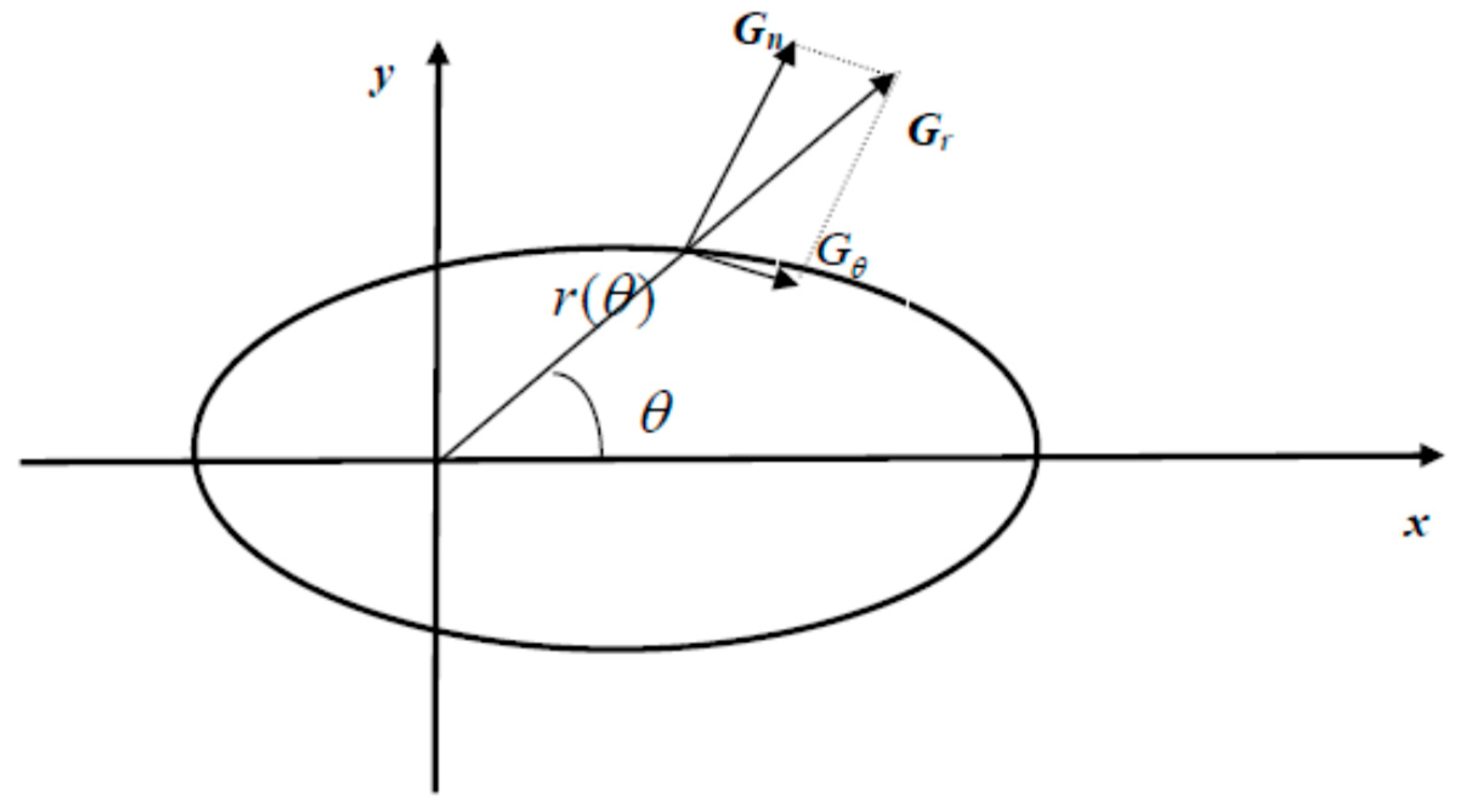
2.1. Mathematical Model

In a temperature gradient, polymers tend to grow anisotropic spherulites. Figure 1 presents the growth model. Here, we assume the temperature gradient is in the x direction and the temperature $T$ obeys linear distribution [18], namely, $T=T_0+\Lambda \cdot x$, where $T_0$ is the central temperature and $\Lambda$ is the temperature gradient. As per Figure 1, the interface between the spherulite and the melt grows normal to itself, with the growth rate given by the local temperature. However, it is possible to attenuate the computation burden by the radial directions instead. The relation between the normal growth rate, $G_n$, and the radial growth rate, $G_r$, is given as follows [16,17]:

$$G_r=G_n\sqrt{1+{\left(\frac{r^{\prime }}{r}\right)}^2}$$

(1)

with

$$r^{\prime }=dr/d\theta$$

(2)

where $r$ and $\theta$ are the space variables in the $r-\theta$ coordinate system.

The normal growth rate, $G_n$, satisfies the well-known Hoffman–Lauritzen equation [18,19]:

$$G_n=G_0\exp \left\{-U^{*}/\left[R_g(T-T_{\infty })\right]\right\}\exp \left\{-K_g/\left[T(T_m^0-T)\right]\right\}$$

(3)

where $U^{*}$ is an energy parameter similar to an apparent activation energy of motion, $R_g$ is the gas constant, $T_{\infty }=T_g-30$ is considered to be the temperature at which no further molecular displacement is possible. $G_0$ and $K_g$ are experimentally determined constants. For a given iPP, the parameters are as follows [18]: $U^{*}=1500 \mathrm{cal}/\mathrm{mol}$, $R_g=8.314472 \mathrm{J}/(\mathrm{mol}\cdot \mathrm{K})$, $T_{\infty }=231.2 \mathrm{K}$, $T_m^0=458.2 \mathrm{K}$. Constants $K_g$ and $G_0$ depend on the regime of crystallization [18]: $K_g=1.47\times {10}^5 {\mathrm{K}}^2,$ $G_0=0.3359 \mathrm{cm}/\mathrm{s}$, ($T\ge {136 }^{\circ }\mathrm{C}$); $K_g=3.3\times {10}^5 {\mathrm{K}}^2,G_0=3249 \mathrm{cm}/\mathrm{s}$, ($T\le {136 }^{\circ }\mathrm{C}$).

Equations (1–3) provide the mathematical model for the growth of a single spherulite. In the crystallization process, all spherulites start to grow from nuclei. The nucleation density, D, is dependent on temperature. For iPP, the following formula is used [18]:

$$D=\exp [111.265-0.2544(T+273.15)]/{\mathrm{mm}}^3$$

(4)

Piorkowska [18] proposed a probabilistic model for polymer crystallization in a gradient temperature field. This model was based on the Avrami equation [20], namely:

$$\alpha =1-\exp \left[-E(x_0,t)\right]$$

(5)

where $\alpha$ is the conversion degree of the melt into the spherulite. Here, $E(x_0,t)$ can be treated as the “extended volume”, which is [18]:

$$E(x_0,t)=2{\displaystyle {\int }_{x_0-r(\pi ,t)}^{x_0+r(0,t)}D\left|x-x_0\right|{\left\{t^2{\left[{\displaystyle {\int }_{x_0}^x{G}_n{(x^{\prime })}^{-1}d{x}^{\prime }}\right]}^{-2}-1\right\}}^{1/2}dx}$$

(6)

where $x_0$ is an arbitrarily chosen point, and t is the time from the beginning of the crystallization. Here, $\left|x-x_0\right|$ is the absolute distance between $x$ and $x_0$. Note that the nucleation density D is a function of the temperature T, and the temperature T is in turn a function of the space variable x andcare should be taken when integrating. The nucleation density is given in Equation (4) and the unit is per mm³.

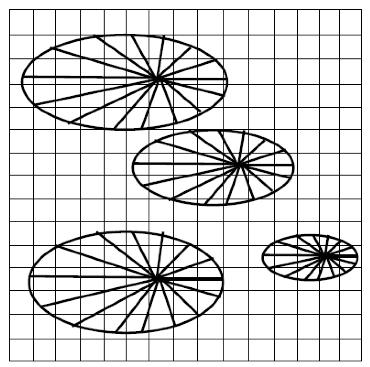
2.2. Numerical Method

The morphological Monte Carlo method [9,11] was used to capture the growth fronts of spherulites. The algorithm is given as follows:

STEP 1: Initialization. The computational zone is divided into several equally sized cells with the total number $N_{tot}$. Each cell is assigned the initial color value 0.

STEP 2: Nucleation. Produce each random nucleus center with a nucleation density D at the beginning of the crystallization, t = 0. Assume that each nucleation unit occupies one cell. Assign different colors to different nuclei in order to distinguish them.

STEP 3: Growth. For each time step $[t_j,t_{j+1}]$, calculate the growth radius r of spherulites according to Equations (1–3). Generate several random points, $N_{rand}$, restricted to the centers of cells. For each random point, if it falls into the radius of one spherulite, it is considered to belong to this spherulite, and the color is assigned to match this spherulite. If a random point falls into the growth radius of more than one spherulite, it is assumed that the point is covered by the first spherulite to reach the point, and the color is assigned to match this spherulite.

STEP 4: Calculate the conversion degree of the melt into spherulites. $\alpha =N_s/N_{tot}$, with $N_s$ being the number of cells that areoccupied by spherulites.

STEP 5: Go to STEP 3 until $t=t_{end}$.

The computational method for the radius r of spherulites should also be presented. As seen in Figure 1, the radius r of spherulites is a function of $\theta$, and this explains why the morphology of spherulites in a gradient temperature field is different from that in a uniform temperature field.

When calculating the radius r of spherulites, a different mesh is used. For each spherulite, we introduce the $\theta$ points at which we will compute the radius r of the spherulite. These points are labeled ${\theta }_0,{\theta }_1,\cdots {\theta }_M$. A uniform grid is used with the step size being $\Delta \theta =2\pi /M$. Therefore, we need to calculate the radius of spherulites $r_0,r_1,\cdots r_M$. From Figure 1, it is obvious that:

$$r_i^{j+1}=r_i^j+G_r\Delta t$$

(7)

where $r_i^{j+1}$ is the radius of spherulites $r_i^{}$ at $t=t_{j+1}$, $r_i^j$ is the radius of spherulites $r_i^{}$ at $t=t_j$, and $\Delta t=t_{j+1}-t_j$ is the time-step size. The radial growth rate, $G_r$, is dependent on the local temperature, and is computed by Equation (1). Then, $r^{\prime }$ is calculated by the finite difference equation [16,17,21], namely:

$${r^{\prime }}_i\approx \{\begin{array}{ll}\frac{r_{i+1}-r_{i-1}}{2\Delta \theta }& i=1,\cdots M-1;\\ \frac{r_1-r_{M-1}}{2\Delta \theta }& i=0,M.\end{array}$$

(8)

Figure 2 shows the schematic representation of two kinds of grid. The square cells are used for Monte Carlo simulation while the unstructured grids are used for prediction ofthe shape evolution of individual spherulites.

3. Results and Discussion

The iPP sample is 600 μm × 600 μm× 11 μm. As this is very thin, it can be treated as essentially two-dimensional. In our simulation, parameters are set as follows: the total number of cells N_tot = 400 × 400, the divisional number in $\theta$ direction M = 500, the total random points $N_{rand}=800000$, the time step size $\Delta t=1 s$ and the initial radius of spherulites $r^0=0$ at $t=0$.

Figure 3 shows the nucleation number and growth rate of spherulites in the iPP sample over the temperature range 105–140 °C. The nucleation number indicates rarity, and the growth rate of spherulites is rather slow when the temperature rises above 130 °C. As the temperature decreases, both the nucleation number and the spherulite growth rate increase. It is obvious from the Figure 3 that the nucleation number increases significantly when the temperature falls below 115 °C.

3.1. Validity of the Morphological Monte CarloMethod

3.1.1. The Growth of a Single Spherulite

Figure 4 shows the growth fronts of a single spherulite with different central temperatures and temperature gradients. Here, the ending time is $t_{end}=12 \min$ and the positions of spherulite growth fronts are plotted at 1-min intervals. The growth fronts of the spherulite are in good agreement with the numerical work of Piorkowska [18] and Liu et al. [12]. Thus, the validity of the morphological Monte Carlo method for capturing the growth front of a single representative spherulite is demonstrated.

As can be seen from Figure 4, the spherulite exhibits anisotropy over the temperature gradient. The growth radius of the spherulite increases on the left side with the lower local temperature, while it is shorter on the right side where the local temperature is higher. The lower central temperature accounts for the longer growth radius of the spherulite. Additionally, the higher temperature gradient supports the longer growth radius of spherulite on the left side and the shorter growth radius on the right side. This is determined by the growth rate of the spherulite expressed by Equation (3). In addition, we can conclude from Figure 4 that the anisotropy of the spherulite can be improved by increasing the central temperature and temperature gradient.

We now discuss the divisional number of $M$ in $\theta$ direction. This value is important since it directly affects the grid to calculate the spherulite size. Figure 5 presents the spherulite shapes at the conditions of $T_0=130 °\mathrm{C}, \Lambda =100 \mathrm{K}/\mathrm{mm}$ predicted with different divisional number of $M$ in $\theta$ direction. When $M$ is small ($M=100$), the growth fronts are not smooth at larger radius of spherulite. This trend improves with the increase of $M$. As shown in Figure 4d, when $M=500$, the smooth growth fronts are obtained. Generally, the larger the $M$, the more accurate the results are. However, the larger $M$ leads to the larger computational cost. Therefore, $M$ should be chosen appropriately. In fact, when simulating the growth of several crystals, due to the impingement, $M$ can be appropriately small.

3.1.2. The Growth of Several Spherulites

Figure 6 describes the crystal morphology evolution with the central temperature of $T_0=132.5 °\mathrm{C}$ and temperature gradient of $\Lambda =35 \mathrm{K}/\mathrm{mm}$. The white region represents the iPP melt, while the colored region represents the spherulites. Different spherulites are distinguished by different colors. The nucleation number is larger on the left (lower local temperature) side, while on the right (higher local temperature) side it is smaller. Due to the fast growth rate at low temperature on the left side, the growth fronts of spherulites impinge on each other and rapidly form the curve boundary. Over time, spherulites with free fronts grow to the right side and form the elongated shapes. These numerical resultsare in good agreement with the experimental results of Piorkowska et al. [22] and the numerical results of Piorkowska [18] and Liu et al. [12]. Thus, our morphological Monte Carlo method is shown to remain effective when capturing the evolution of several spherulites.

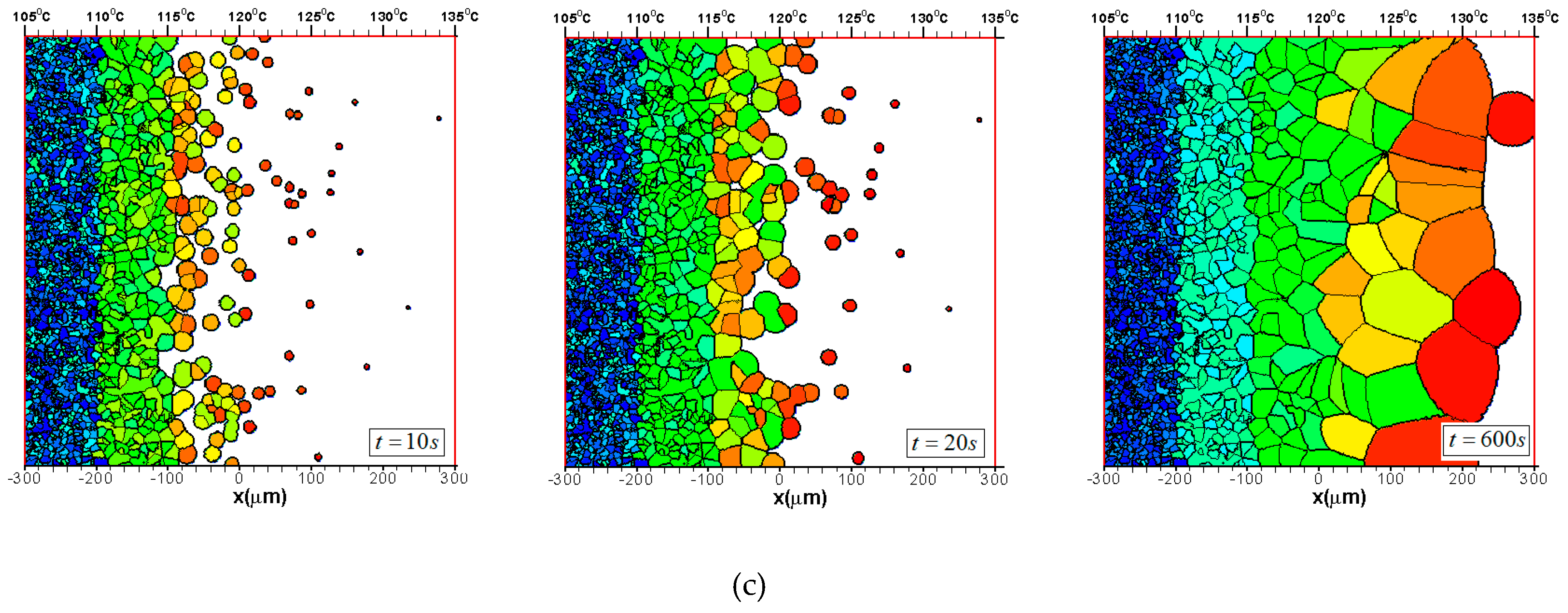
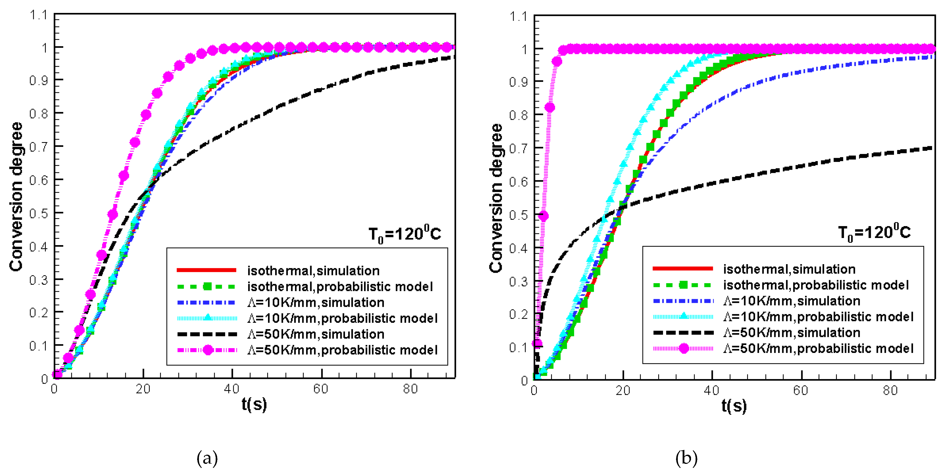
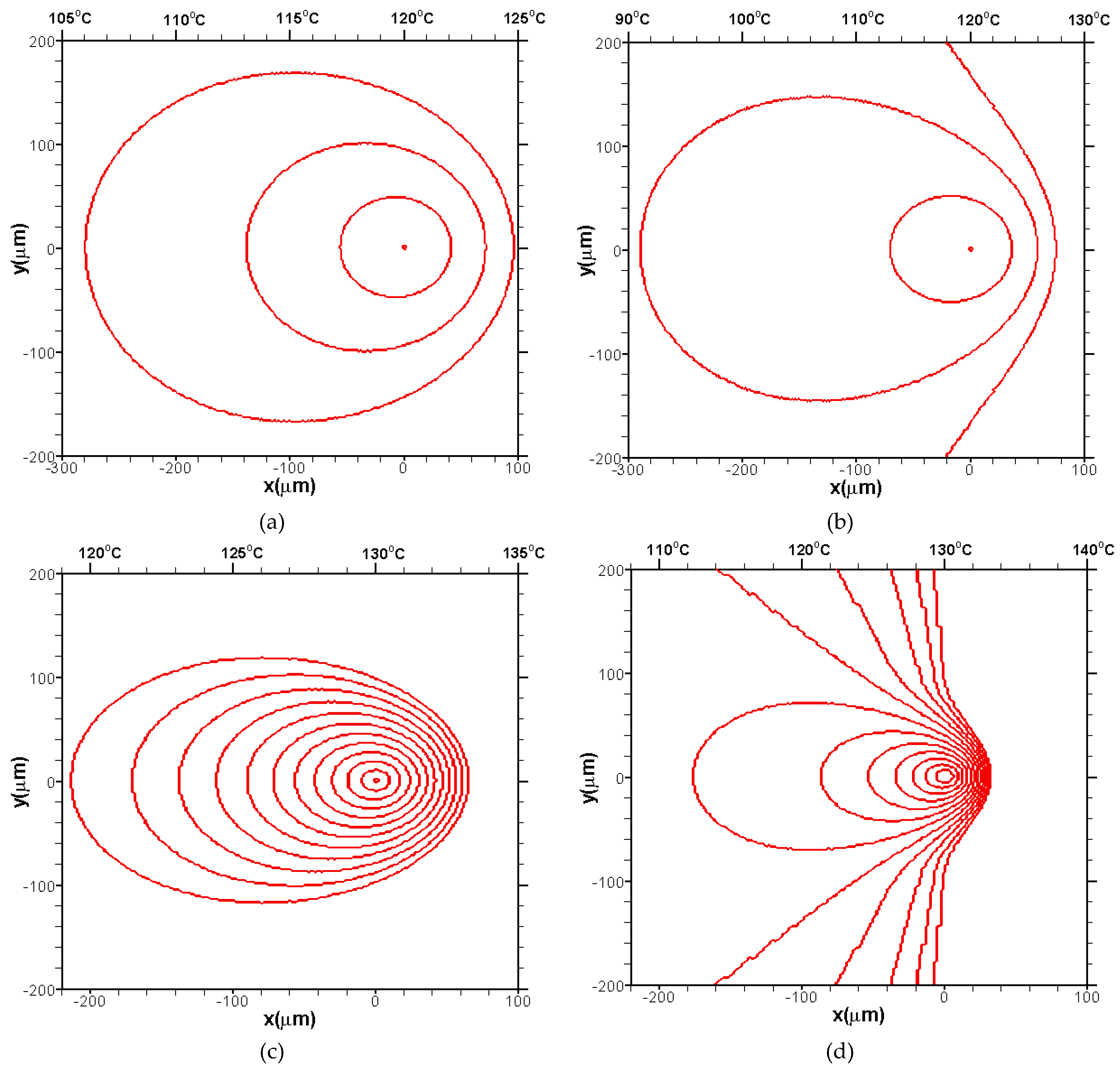
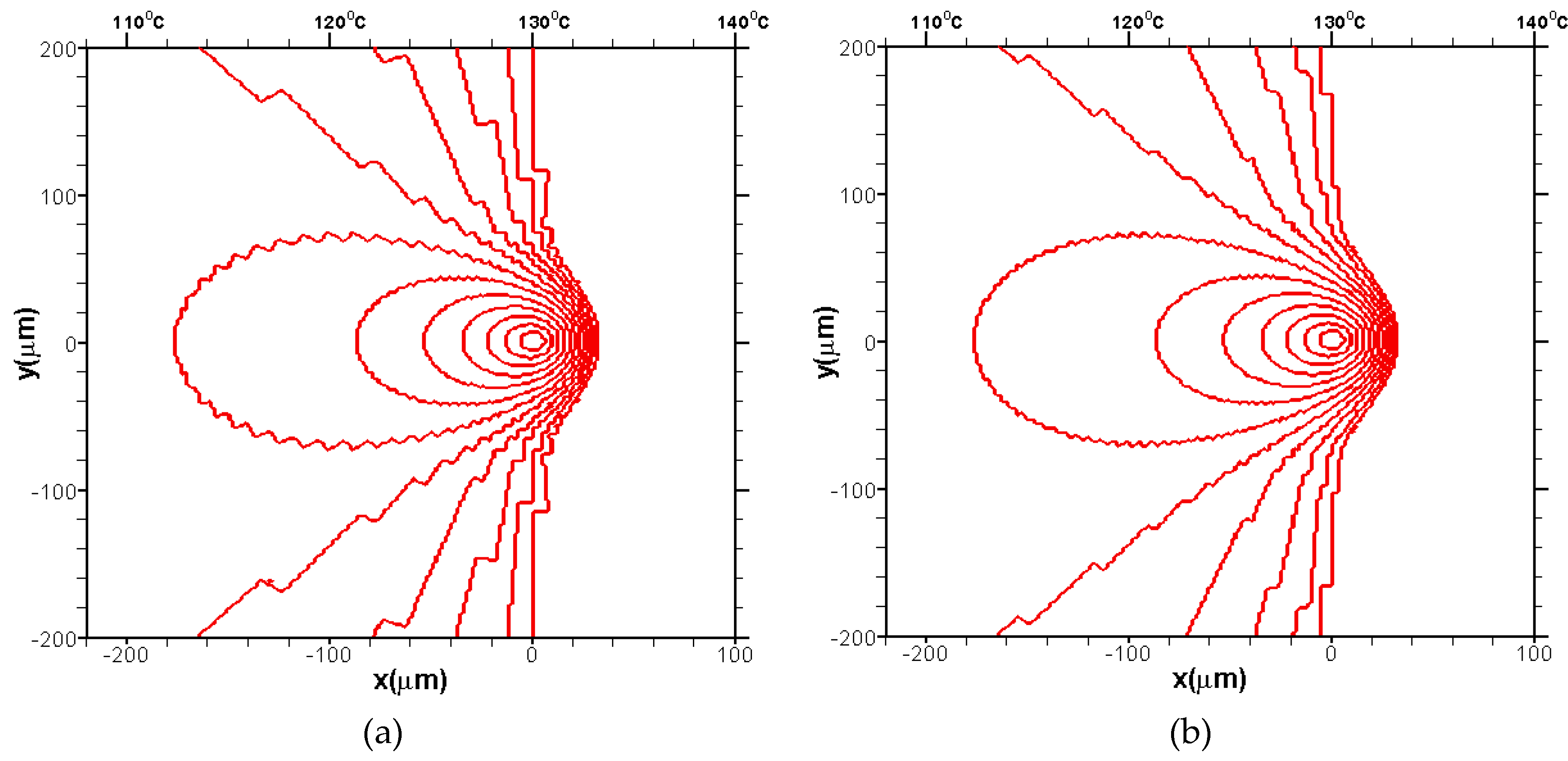
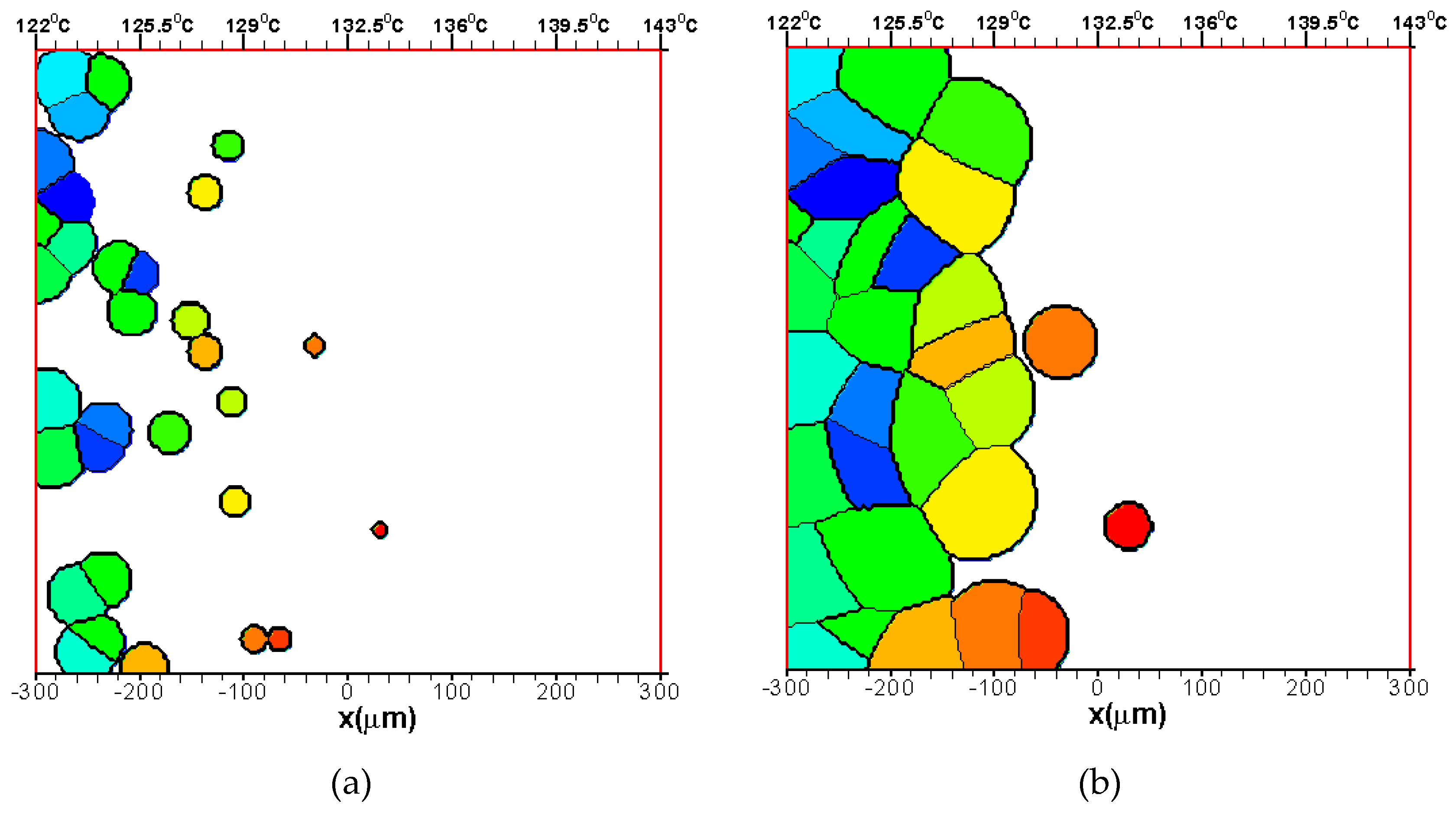
3.2. Effects of CentralTtemperature and Temperature Gradient

Figure 7 and Figure 8 show the morphologyevolution of spherulites with different central temperatures and temperature gradients. Under the isothermal condition ($\Lambda =0 \mathrm{K}/\mathrm{mm}$), the growth fronts of spherulites are isotropic and form a straight line boundary when impingement occurs, while in the temperature gradient field, the growth fronts of spherulites are anisotropic and form a curvilinear boundary when impingement occurs [3]. The curvature of the boundary increases with an increase in central temperature and temperature gradient. The impinged boundary is nearly parallel to the temperature gradient and the growth fronts are nearly perpendicular to the temperature gradient under conditions of higher central temperature and higher temperature gradient. Additionally, the spherulites are elongated in these cases, and the anisotropy is pronounced. This is because on the left (lower temperature) side, the spherulites can grow faster but soon impinge on each other, while on the right (higher temperature) side, the spherulites grow more slowly and have enough space to grow due to the rare nucleation number. The observed tendency is consistent with the numerical works of Piorkowska [18].

Figure 9 and Figure 10 show the comparison of the conversion degree of the melt into spherulites at isotherms of 125 °C and 120 °C under different temperature gradients. Two different representative volume element (RVE) sizes are used to calculate the conversion degree, namely, $[-100 \mathsf{\mu }\mathrm{m}, 100 \mathsf{\mu }\mathrm{m}]$ and $[-300 \mathsf{\mu }\mathrm{m}, 300 \mathsf{\mu }\mathrm{m}]$. Here, the simulation results are obtained by the fraction of crystals (see Section 2.2, morphological Monte Carlo method, STEP 4). The analytical results are obtained by the probabilistic model set out in Equations (5) and (6).

It can be seen from Figure 9 and Figure 10 that in the isothermal crystallization, the results obtained by the morphological Monte Carlo method are in good agreement with the analytical solution. However, with an increase in the temperature gradient, the deviations between these results gradually increase. Under a temperature gradient of $\Lambda =50 \mathrm{K}/\mathrm{mm}$, there is a significant difference between them. The explanation for the simulation results is as follows: The higher temperature gradient leads to a lower temperature on the left side and a higher temperature on the right side. As the lower temperature is favorable for nucleation and the growth of spherulites, and the higher temperature is not conducive to the formation of spherulites, there is a segmentation at $\alpha \approx 0.5$. However, in the probabilistic model, the conversion degree is determined by the “extended volume,” calculated by all spherulites growing unrestricted (without considering the impingement or growth outside the computational zone). Due to the higher temperature gradient, the largerextended volume is obtained on the colder side, and its contribution to the total extended volume will be much more significant than that of the smaller extended volume on the hotter side. Thus, the higher the temperature gradient, the larger the conversion degree. This is inconsistent with our Monte Carlo simulation results.

Piorkowska [18] compared the solution for the probabilistic model with the experimental data when the central temperature was higher than 130 °C, and concluded that increasing the temperature gradient would accelerate the conversion degree of the melt into spherulites. From Figure 4 and Figure 6, we speculate that this is because the nucleation number on the right side is nearly 0 when the central temperature is above 130 °C. Under a higher temperature gradient, the nucleation number and the spherulites with free growth fronts increase significantly on the left side. These crystals can extend from the left side to the right side. Although the growth rate of spherulites is smaller due to the higher local temperature on the right side, it can also contribute to the overall crystallization kinetics. However, when the central temperature is lower than 125 °C, and when there is a higher temperature gradient, the nucleation is weaker and the growth rate of spherulites is slower on the right side, leading to a decrease in the crystallization rate as shown in Figure 9 and Figure 10.

Therefore, it can be concluded that the probabilistic model is not suitable to calculate the conversion degree of the melt into spherulites in the high temperature gradient field (e.g., $\Lambda =50 \mathrm{K}/\mathrm{mm}$) when the central temperature is below 125 °C.

Figure 9 and Figure 10 also show us that the lower the central temperature, the higher the conversion degree of the melt into spherulites.

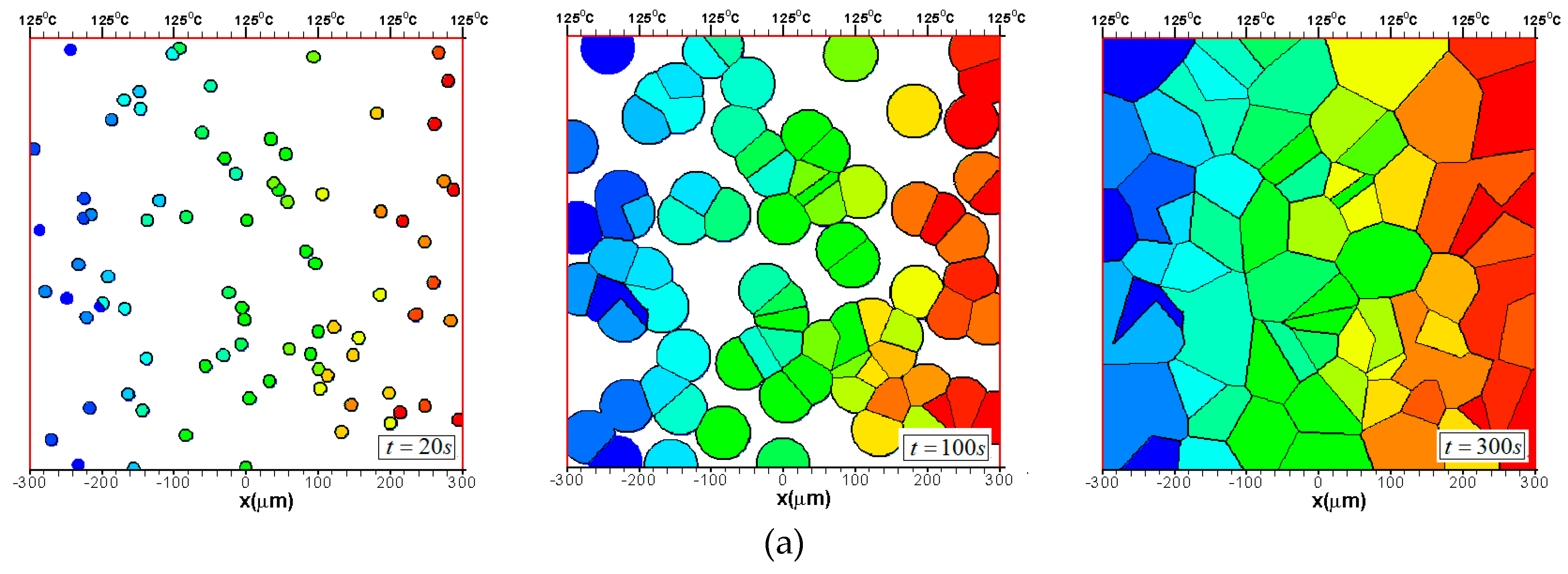
3.3. Difference Between IsothermalCcrystallization and Crystallization in a Temperature Gradient

In the multiscale simulation, there are two kinds of temperature and crystal morphology models in a control volume: one is to treat the temperature as a uniform field (e.g., temperature on the central vertex of the control volume) and apply the isotropic spherulites model [8,10], and the other is to assume the temperature with a linear gradient and apply the anisotropic spherulites model [13,15]. Although the latter is more accurate, it is both more algorithmically complex and more computationally expensive.

The coupling between meso- and macro-scale is realized by the conversion degree of the melt into spherulites in the multiscale simulation [10,15]. Therefore, it is necessary to study whether the crystallization in a temperature gradient can be simplified as isothermal crystallization given the conversion degree error remains within a certain value. This work can provide useful data to support the multiscale simulation. It should be noted that in the multiscale simulation, the temperature in a control volume changes with time (non-isothermal). However, the non-isothermal condition can be treated as the accumulation of multiple isothermal conditions, accounting for the continuing significance of this work.

We define the following errors, namely:

$$L_1-error=\frac{1}{t_{end}}{\displaystyle {\int }_0^{t_{end}}\left|{\alpha }_{\Lambda }-{\alpha }_{iso}\right|dt}$$

(9)

where ${\alpha }_{\Lambda }$ is the conversion degree ofthe melt into spherulites in a temperature gradient, ${\alpha }_{iso}$ is the conversion degree of the melt into spherulites in isothermal crystallization, and $t_{end}$ is the ending time. The conversion degree at isothermals of central temperature is used. The volume used for calculation is $[-100 \mathsf{\mu }\mathrm{m}, 100 \mathsf{\mu }\mathrm{m}]$.

Table 1. Maximum temperature gradient under different central temperature.

${\mathit{T}}_0$	${\mathit{L}}_1-\mathit{e}\mathit{r}\mathit{r}\mathit{o}\mathit{r}$	${\mathbf{\Lambda }}_{\mathbf{max}}$	${\mathit{L}}_1-\mathit{e}\mathit{r}\mathit{r}\mathit{o}\mathit{r}$	${\mathbf{\Lambda }}_{\mathbf{max}}$
125 °C	2.1%	15 K/mm	5.1%	27 K/mm
120 °C	1.6%	18 K/mm	5.0%	30 K/mm
115 °C	1.5%	30 K/mm	5.0%	45 K/mm
110 °C	1.5%	31 K/mm	5.0%	48 K/mm
105 °C	2.2%	40 K/mm	3.8%	50 K/mm

lists the maximum temperature gradient ${\Lambda }_{\max }$ under different central temperatures when $L_1-error$ is less than 2% and less than 5%. Withan increase in central temperature, the maximum temperature gradient decreases. When the central temperature is lower than 125 °C, the temperature gradient should not be higher than 15 K/mm and 27 K/mm if $L_1-error$ is set as 2% and 5%, respectively. Therefore, crystallization in these temperature gradient conditions can be simplified as isothermal crystallization. The effects of temperature gradients should be taken into account, under other conditions.

Since the conversion degree of the melt into spherulites is not the only quantity to analyze by comparing isothermal crystallization and the crystallization in a temperature gradient, we now define the anisotropy of the spherulite. As illustrated in Figure 1, spherulites grow anisotropically from the nucleus center. Spherulite asymmetry is defined as follows:

$$S=\frac{{\overline{r}}_0}{{\overline{r}}_{M/2}}$$

(10)

where ${\overline{r}}_0$ is the averageradius of spherulite at $\theta =0$ and ${\overline{r}}_{M/2}$ is the average radius of spherulite at $\theta =\pi$. Note that here the average radius of spherulite is calculated by the final morphology, considering the impingement.

Table 2. Spherulite asymmetryerror under different central temperature and different temperature gradients.

${\mathit{T}}_0$	$\mathbf{\Lambda }$	$({\mathit{S}}_{\mathbf{\Lambda }}-{\mathit{S}}_{\mathit{i}\mathit{s}\mathit{o}})/{\mathit{S}}_{\mathit{i}\mathit{s}\mathit{o}}$	$\mathbf{\Lambda }$	$({\mathit{S}}_{\mathbf{\Lambda }}-{\mathit{S}}_{\mathit{i}\mathit{s}\mathit{o}})/{\mathit{S}}_{\mathit{i}\mathit{s}\mathit{o}}$
125 °C	15 K/mm	8.8%	27 K/mm	14.2%
120 °C	18 K/mm	3.5%	30 K/mm	6.6%
115 °C	30 K/mm	3.0%	45 K/mm	4.2%
110 °C	31 K/mm	2.4%	48 K/mm	3.0%
105 °C	40 K/mm	2.0%	50 K/mm	2.5%

lists the spherulite asymmetry error under different central temperature and different temperature gradients. Here, $S_{\Lambda }$ is the spherulite asymmetry in temperature gradients and $S_{iso}$ is the spherulite asymmetry with isothermal crystallization. It is obvious that with a decrease in central temperature, the spherulite asymmetry error decreases.

4. Conclusions

In this paper, the morphological Monte Carlo method for simulating the anisotropic growth of spherulites for iPP in a temperature gradient field is presented. The evolution of spherulites and the development of the conversion degree of the melt into spherulites under different central temperatures and temperature gradients are analyzed. Conclusions are drawn as follows:

(1) The morphological Monte Carlo method presented here is valid and effective. It is capable of not only successfully capturing the growth fronts of anisotropic spherulites, but also accurately predicting the conversion degree of the melt into spherulites.

(2) High central temperature and high temperature gradient can improve the anisotropy of spherulites.

(3) When the central temperature is lower than 125 °C and the temperature gradient is high, the probabilistic model is not suitable to predict the conversion degree of the melt into spherulites.

(4) When the temperature gradient is less than 15 K/mm and 27 K/mm, the error in conversion degree of the melt into spherulites is controlled within 2% and 5%, respectively, which can be simplified as isothermal crystallization.

We present a morphological Monte Carlo simulation for the anisotropic growth of spherulites for iPP in a temperature gradient. The proposed modelling method can be easily extended to the study of different polymers when the nucleation formula and the growth rate formula are known. The athermal nucleation [23] model can also be applied. We hope the method and the results presented here can give more insight about the polymer crystallization in industrial processes.

References

1. Kennedy, P.; Zheng, R. Flow Analysis of Injection Molds; Munich Carl Hanser Verlag: Munich, Germany, 2013. [Google Scholar]
2. Pantanin, R.; Coccorullo, I.; Speranza, V.; Titomanlio, G. Modeling of morphology evolution in the injection molding process of thermoplastic polymers. Prog. Polym. Sci. 2005, 30, 1185–1222. [Google Scholar] [CrossRef]
3. Piorkowska, E.; Galeski, A. Handbook of Polymer Crystallization; Wiley: New Jersey, NJ, USA, 2013. [Google Scholar]
4. Raabe, D. Mesoscale simulation of spherulite growth during polymer crystallization by use of a cellular automaton. Acta Mater. 2004, 52, 2653–2664. [Google Scholar] [CrossRef]
5. Raabe, D.; Godara, A. Mesoscale simulation of the kinetics and topology of spherulite growth during crystallization of isotactic polypropylene (iPP) by using a cellular automaton. Modell. Simul. Mater. Sci. Eng. 2005, 13, 733–751. [Google Scholar] [CrossRef]
6. Capasso, V. Mathematical Modeling for Polymer Processing; Springer: Berlin, Germany, 2002. [Google Scholar]
7. Micheletti, A.; Burger, M. Stochastic and deterministic simulation of nonisothermal crystallization of polymers. J. Math. Chem. 2001, 30, 169–193. [Google Scholar] [CrossRef]
8. Ruan, C.; Ouyang, J.; Liu, S. Multi-scale modeling and simulation of crystallization during cooling in short fiber reinforced composites. Int. J. Heat Mass Transfer. 2012, 55, 1911–1921. [Google Scholar] [CrossRef]
9. Ruan, C. Kinetics and morphology of flow induced polymer crystallization in 3D shear flow investigated by Monte Carlo simulation. Crystals 2017, 7, 51. [Google Scholar] [CrossRef]
10. Ruan, C.; Liang, K.; Liu, E. Macro-micro simulation for polymer crystallization in Couette flow. Polymers 2017, 9, 699. [Google Scholar] [CrossRef] [PubMed]
11. Ruan, C.; Liu, C.; Zheng, G. Monte carlo simulation for the morphology and kinetics of spherulites and shish-kebabs in isothermal polymer crystallization. Math. Prob. Eng. 2015, 50624, 1–10. [Google Scholar] [CrossRef]
12. Liu, Z.; Ouyang, J.; Ruan, C.; Liu, Q. Simulation of polymer crystallization under isothermal and temperature gradient conditions using praticle level set method. Crystals 2016, 6, 90. [Google Scholar] [CrossRef]
13. Liu, Z.; Ouyang, J.; Zhou, W.; Wang, X.D. Numerical simulation of the polymer crystallization during cooling stage by using level set method. Comput. Mater. Sci 2015, 97, 245–253. [Google Scholar] [CrossRef]
14. Wang, X.; Ouyang, J.; Zhou, W.; Liu, Z. A phase field technique for modeling and predicting flow induced crystallization morphology of semi-crystalline polymers. Polymers 2016, 8, 230. [Google Scholar] [CrossRef]
15. Charbon, C.; Swaminarayar, S. A multiscale model for polymer crystallization. II: Solidification of a macroscopic part. Polym. Eng. Sci. 1998, 38, 644–656. [Google Scholar] [CrossRef]
16. Swaminarayan, S.; Charbon, C. A multiscale model for polymer crystallization. I. growth of individual spherulites. Polym. Eng. Sci. 1998, 38, 634–643. [Google Scholar] [CrossRef]
17. Thananchai, L. Mathematical modeling of solidification of semi-crystalline polymers under quiescent non-isothermal crystallization: Determination of crystallite’s size. Sci. Asia. 2001, 27, 127–132. [Google Scholar]
18. Piorkowska, E. Modeling of polymer crystallization in a temperature gradient. J. Appl. Polym. Sci 2002, 86, 1351–1362. [Google Scholar] [CrossRef]
19. Hoffman, J.D.; Miller, R.L. Kinetics of crystallization from the melt and chain folding in polyethylene fractions revisited: theory and experiment. Polymer 1997, 38, 3151–3212. [Google Scholar] [CrossRef]
20. Avrami, M. Kinetics of phase change. I. General theory. J. Chem. Phys. 1939, 7, 1103–1112. [Google Scholar]
21. Mark, H. Introduction to Numerical Methods in Differential Equations; Springer: Berlin, Germany, 2011. [Google Scholar]
22. Pawlak, A.; Piorkowska, E. Crystallization of isotactic polypropylene in a temperature gradient. Colloid. Polym. Sci. 2001, 279, 939–946. [Google Scholar] [CrossRef]
23. Ziabicki, A. Crystallization of polymers in variable external conditions. Colloid. Polym. Sci. 1996, 274, 705–716. [Google Scholar] [CrossRef]
Figure 1. Geometric interpretation of the relation between the normal growth rate G n and radial growth rate G r .
Crystals 09 00213 g001
Figure 2. Schematic representation of square cells and unstructured grids: the square cells are used for Monte Carlo simulation, the unstructured grids are used for prediction the shape evolution of spherulites.
Crystals 09 00213 g002
Figure 3. Nucleation number and growth rate for isotactic polypropylene (iPP) over the temperature range 105–140 °C.
Crystals 09 00213 g003
Figure 4. Spherulite shapes predicted by morphological Monte Carlo method: (a) T 0 = 120   ° C ,   Λ = 50   K / mm , (b) T 0 = 120   ° C ,   Λ = 100   K / mm , (c) T 0 = 130   ° C ,   Λ = 50   K / mm , (d) T 0 = 130   ° C ,   Λ = 100   K / mm .
Crystals 09 00213 g004
Figure 5. Spherulite shapes ( T 0 = 130   ° C ,   Λ = 100   K / mm ) predicted with different divisional number of M in θ direction: (a) M = 100 , (b) M = 200 .
Crystals 09 00213 g005
Figure 6. Spherulite shapes predicted by morphological Monte Carlo method: (a) t = 2   min , (b) t = 6   min , (c) t = 15   min , (d) t = 60   min .
Crystals 09 00213 g006aCrystals 09 00213 g006b
Figure 7. Morphology evolution with the central temperature T 0 = 125   ° C : (a) isothermal ( Λ = 0   K / mm ), (b) Λ = 10   K / mm , (c) Λ = 50   K / mm .
Crystals 09 00213 g007aCrystals 09 00213 g007b
Figure 8. Morphology evolution with the central temperature T 0 = 120   ° C : (a) isothermal ( Λ = 0   K / mm ), (b) Λ = 10   K / mm , (c) Λ = 50   K / mm .
Crystals 09 00213 g008aCrystals 09 00213 g008b
Figure 9. Conversion degree of the melt into spherulites at isothermals of T 0 = 125   ° C : (a) [ 100   μ m ,   100   μ m ] , (b) [ 300   μ m ,   300   μ m ] .
Crystals 09 00213 g009
Figure 10. Conversion degree of the melt into spherulites at isothermals of T 0 = 120   ° C : (a) [ 100   μ m ,   100   μ m ] , (b) [ 300   μ m ,   300   μ m ] .
Crystals 09 00213 g010