Article

Generalization of the Unified Analytic Melt-Shear Model to Multi-Phase Materials: Molybdenum as an Example

1
Theoretical Division, Los Alamos National Laboratory, Los Alamos, NM 87545, USA
2
Computational Physics Division, Los Alamos National Laboratory, Los Alamos, NM 87545, USA
3
Physics Division, Los Alamos National Laboratory, Los Alamos, NM 87545, USA
*
Author to whom correspondence should be addressed.
Crystals 2019, 9(2), 86; https://doi.org/10.3390/cryst9020086
Submission received: 21 November 2018 / Revised: 23 January 2019 / Accepted: 24 January 2019 / Published: 6 February 2019

Abstract

:
The unified analytic melt-shear model that we introduced a decade ago is generalized to multi-phase materials. A new scheme for calculating the values of the model parameters for both the cold ( T = 0 ) shear modulus ( G ) and the melting temperature at all densities ( ρ ) is developed. The generalized melt-shear model is applied to molybdenum, a multi-phase material with a body-centered cubic (bcc) structure at low ρ which loses its dynamical stability with increasing pressure (P) and is therefore replaced by another (dynamically stable) solid structure at high ρ . One of the candidates for the high- ρ structure of Mo is face-centered cubic (fcc). The model is compared to (i) our ab initio results on the cold shear modulus of both bcc-Mo and fcc-Mo as a function of ρ , and (ii) the available theoretical results on the melting of bcc-Mo and our own quantum molecular dynamics (QMD) simulations of one melting point of fcc-Mo. Our generalized model of G ( ρ , T ) is used to calculate the shear modulus of bcc-Mo along its principal Hugoniot. It predicts that G of bcc-Mo increases with P up to ∼240 GPa and then decreases at higher P. This behavior is intrinsic to bcc-Mo and does not require the introduction of another solid phase such as Phase II suggested by Errandonea et al. Generalized melt-shear models for Ta and W also predict an increase in G followed by a decrease along the principal Hugoniot, hence this behavior may be typical for transition metals with ambient bcc structure that dynamically destabilize at high P. Thus, we concur with the conclusion reached in several recent papers (Nguyen et al., Zhang et al., Wang et al.) that no solid-solid phase transition can be definitively inferred on the basis of sound velocity data from shock experiments on Mo. Finally, our QMD simulations support the validity of the phase diagram of Mo suggested by Zeng et al.

1. Introduction: Unified Analytic Melt-Shear Model

A reliable model of the adiabatic (isentropic) shear modulus ( G ) of a polycrystalline solid at all temperatures from zero to close to T m , the melting temperature, and up to pressures ( P ) of order 100 GPa is needed for many applications, including the modeling of plastic deformation at extremes of pressure and temperature, numerical calculations of elastic and shock wave propagation, and even calculations of the oscillations of low-mass astrophysical objects. In 2003–2004 we developed a unified analytic model for the melting temperature as a function of density, T m ( ρ ) , and the density-temperature dependence of the shear modulus, G ( ρ , T ) , at all densities and 0 T T m [1,2]. The model for T m ( ρ ) is based in part on our analytic model for the Grüneisen parameter,
γ ( ρ ) = 1 2 + γ 1 ρ 1 / 3 + γ 2 ρ q ,
where the parameters γ 1 , γ 2 , and q can be determined from ambient data by solving a system of three algebraic equations [1,2]. Equation (1) in conjunction with the Lindemann melting criterion [3] yields
T m ( ρ ) = T m ( ρ r e f ) ρ ρ r e f 1 / 3 exp 6 γ 1 1 ρ r e f 1 / 3 1 ρ 1 / 3 + 2 γ 2 q 1 ρ r e f q 1 ρ q ,
where ρ r e f is a conveniently chosen reference density. The melting temperature and shear modulus along the solidus approximately satisfy the relation [1,4,5]
G ( ρ , T m ( ρ ) ) ρ T m ( ρ ) = G ( ρ r e f , T m ( ρ r e f ) ) ρ r e f T m ( ρ r e f ) .
Preston and Wallace [6] modeled G ( ρ , T ) as a linear function of the reduced temperature T / T m with the correct value G ( ρ , 0 ) at T = 0 :
G ( ρ , T ) = G ( ρ , 0 ) 1 β T T m ( ρ ) .
The thermoelastic softening parameter β may be density dependent. Combining Equations (2)–(4) results in
G ( ρ , 0 ) = G ( ρ r e f , 0 ) ρ ρ r e f 4 / 3 exp 6 γ 1 1 ρ r e f 1 / 3 1 ρ 1 / 3 + 2 γ 2 q 1 ρ r e f q 1 ρ q .
Equations (2), (4), and (5) constitute our unified model of T m ( ρ ) and G ( ρ , T ) for single-phase metals.
For polymorphic (multi-phase) metals, the γ 1 - γ 2 -q values for the ambient solid structure may differ significantly from those for the high-P structure(s), and therefore the model may fail in its description of those high-P structure(s). Here we generalize our unified melt-shear model to polymorphic materials. Let G i ( ρ , 0 ) be the cold shear modulus of phase i, and similarly let T m i ( ρ ) denote the melting curve of phase i. In our multi-phase model both G ( ρ , 0 ) and T m ( ρ ) are accurate envelopes of the G i ( ρ , 0 ) and T m i ( ρ ) . We shall explain how such envelopes are constructed, and demonstrate the fidelity of the generalized model using molybdenum as an example.

2. Molybdenum: An Example of a Multi-Phase Material

Molybdenum is one of the most important technological materials. Although its phase diagram is not known in detail, there are several features of the phase diagram that have been firmly established. First, melting on the shock Hugoniot of Mo occurs at ∼400 GPa [7,8,9], and presumably at T 10,000 K [7]. Second, the stability of body-centered cubic (bcc) Mo has been confirmed experimentally to 560 GPa under room-T isothermal compression [10], and to 1000 GPa under ramp-wave compression [11]. There is presently no experimental evidence for a solid-solid (s-s) transition in Mo. However, there is compelling theoretical evidence for a s-s phase transition at high pressures [12,13,14,15,16]. Our calculations of the phonon spectrum of bcc-Mo presented below (see Figure 1) clearly show its dynamic instability at 1000 GPa and low T, and previous simulations indicated that bcc-Mo dynamically destabilizes at ∼700 GPa [17,18]. Hence, a s-s phase transformation to another solid phase that is dynamically stable is expected to occur at ∼700 GPa at low T. Two candidates for the high-P structure of Mo are face-centered cubic (fcc) [17,19,20] and double hexagonal close-packed (dhcp) [12,18,21]. Simulations show that the bcc-fcc (bcc-dhcp) phase boundary has positive slope at P 700 GPa [12,17]. We emphasize that this theoretical phase boundary is consistent with the aforementioned experimental results for room-T isothermal compression to 560 GPa, and with ramp-wave compression to 1000 GPa. The ramp-wave trajectory (RWT) in the P-T plane has a positive slope and lies at sufficiently high temperatures that the bcc-fcc (bcc-dhcp) transition boundary lies below the RWT; e.g., T 5000 K on the RWT at 700 GPa [11], and at 800 GPa the bcc-fcc transition is predicted to occur at ∼5000 K [17] or ∼4500 K [12], while T 6500 K on the RWT [11]. Therefore at P 700 GPa the crystal structure is bcc from 0 to T m , and is also bcc at high T to at least 1000 GPa.
For our present purposes of demonstrating the generalization of the unified melt-shear model, it is not essential to definitively identify the high-P structure (fcc or dhcp). Numerous examples show that the elastic properties of different hexagonal arrangements of the same material (AB for hcp, ABC for fcc, ABAC for dhcp, etc., where A, B and C denote the layer stacking in the unit cell) are very close to each other; e.g., the results of [22] reveal that the shear moduli of both hcp-Be and fcc-Be are virtually identical, and so are the corresponding melting curves [23]. Hence, we expect both the shear moduli and the melting curves of fcc-Mo and dhcp-Mo to be close to each other. Although our QMD simulations strongly suggest that the high-density phase of Mo is dhcp, simply because fcc elastic constants are generally easier to calculate than the dhcp ones, for the purpose of comparing our ab initio results to the new generalized melt-shear model here we assume that the high-P structure of Mo is fcc.
An analysis of longitudinal sound speed data along the principal Hugoniot of Mo by Errandonea et al. [24] shows a decrease in the shear modulus with increasing pressure. They concluded that such behavior is indicative of a transformation of bcc-Mo into another solid phase. However, the conclusion of earlier theoretical work by Cazorla et al. [25] and Zeng et al. [17] is that there is no s-s phase transformation on the Mo Hugoniot. More recent calculations of C L along the Hugoniot in bcc-Mo by Lukinov et al. [16] again suggests that a s-s transition occurs at ∼200 GPa. However, we have carefully analyzed the calculations of Lukinov et al., and we find that their conclusion is incorrect. We maintain that a s-s transition along the Mo Hugoniot is ruled out by both experiment and theory. A detailed discussion of the experimental and theoretical/computational investigations of a possible s-s transition on the Mo Hugoniot is presented in Appendix A.
In the following we construct a thermoelasticity model for bcc-Mo that predicts a decrease in G with P on the principal Hugoniot at pressures above ∼240 GPa, hence the decrease in G with P is not evidence for another solid phase of Mo. Thus our model supports the conclusion of References [8,9,26] that no s-s phase transition should be inferred from the sound velocity data on Mo.

3. Generalization of the Unified Melt-Shear Model to Multi-Phase Materials

As mentioned above, the unified melt-shear model [1,2] is based on the simplifying approximation that both G ( ρ , 0 ) and T m ( ρ ) are related to a common Grüneisen parameter. In the general case, this approximation may fail. Indeed, since G ( ρ , 0 ) Θ D 2 ( 3 , ρ ) ρ 1 / 3 [27,28],
d ln G ( ρ , 0 ) d ln ρ 2 γ ( 3 , ρ ) + 1 3 , γ ( 3 , ρ ) d ln Θ D ( 3 , ρ ) d ln ρ .
Similarly, since in the Lindemann formulation T m ( ρ ) Θ D 2 ( 2 , ρ ) ρ 2 / 3 [27,28],
d ln T m ( ρ ) d ln ρ 2 γ ( 2 , ρ ) 2 3 , γ ( 2 , ρ ) d ln Θ D ( 2 , ρ ) d ln ρ .
In the above equations, Θ D ( n , ρ ) ω i n 1 / n / k B , n 3 are the Debye characteristic temperatures [28]. As noted in [27], Wallace argued that Θ D ( 0 , ρ ) should be used in the Lindemann melting formula, Equation (7), instead of Θ D ( 2 , ρ ) . The two gammas appearing in Equations (6) and (7) must asymptote to 1/2 as ρ [1,2,28]. For single-phase materials they are approximately equal at all densities and are accurately modeled as γ ( ρ ) = 1 / 2 + γ 1 / ρ 1 / 3 + γ 2 / ρ q [29]. However, this approximate equality of γ ( 3 , ρ ) and γ ( 2 , ρ ) most likely fails for multi-phase materials having solid phases that dynamically stabilize (or destabilize) at elevated P . For example, consider a high-P solid structure stable at low T but unstable at high T , and assume that the s-s phase boundary has a positive slope. Then there is a range of P in which the cold shear modulus exists and is described by Equation (6), but T m does not exist for this high-P phase since the material melts from another stable solid phase. The same Grüneisen gamma cannot be used for both G ( ρ , 0 ) and T m ( ρ ) . If the solid-solid boundary has negative slope then there is a range of P for which T m exists and is described by Equation (7) but the cold shear modulus does not exist, and again a single Grüneisen gamma cannot be used for both cold G and T m .
In such cases we assume that both G ( ρ , 0 ) and T m ( ρ ) can be constructed as the envelopes of the G i ( ρ , 0 ) and T m i ( ρ ) for a sequence of solid phases, but they are not necessarily coupled to each other in terms of a common set of parameters. We introduce the corresponding two Grüneisen gammas, γ G ( ρ ) and γ T m ( ρ ) , so that Equations (6) and (7) are generalized to
d ln G ( ρ , 0 ) d ln ρ 2 γ G ( ρ ) + 1 3 ,
d ln T m ( ρ ) d ln ρ 2 γ T m ( ρ ) 2 3 .
Using the approach developed in [2], it is easy to show that both gammas must be analytic functions of ρ 1 / 3 , essentially the interatomic distance. Since both gammas asymptote to 1/2 as ρ ,
γ G ( ρ ) = 1 2 + i = 1 g G i ρ 1 / 3 i 1 2 + γ 1 , G ρ 1 / 3 + γ 2 ρ q 2 ,
γ T m ( ρ ) = 1 2 + i = 1 g T m i ρ 1 / 3 i 1 2 + γ 1 , T m ρ 1 / 3 + γ 3 ρ q 3 .
Below we show that γ 1 is common to both G and T m , and that
γ 1 , G γ 1 , T m γ 1 = 7 40 Z 2 / 3 ,
where Z is the atomic number of the material. In Equations (10) and (11) the terms γ 2 / ρ q 2 and γ 3 / ρ q 3 represent the contributions of the quadratic and higher-order terms. Note that since these equations are meant to describe the envelopes of the G i ( ρ , 0 ) and T m i ( ρ ) for each of the stable solid phases of the material, the signs in front of the terms g G i / ρ i / 3 and g T m i / ρ i / 3 can in principle be arbitrary, and so may be the signs of both γ 2 and γ 3 . Based on general grounds, however, we expect that both q 2 and q 3 are positive.
With Equations (10)–(12) it follows from Equations (8) and (9) that
G ( ρ , 0 ) = G ( ρ 0 , 0 ) ρ ρ 0 4 / 3 exp 6 γ 1 1 ρ 0 1 / 3 1 ρ 1 / 3 + 2 γ 2 q 2 1 ρ 0 q 2 1 ρ q 2 ,
T m ( ρ ) = T m ( ρ m ) ρ ρ m 1 / 3 exp 6 γ 1 1 ρ m 1 / 3 1 ρ 1 / 3 + 2 γ 3 q 3 1 ρ m q 3 1 ρ q 3 ,
where ρ 0 and ρ m are the corresponding initial densities, usually taken as those at ambient P.

The Value of γ 1 : Ultrahigh Density Limit

The value of γ 1 is found in the limit of ultrahigh densities. In this limit, it follows from Thomas-Fermi theory that P / Z 10 / 3 , B / Z 10 / 3 , and G / Z 10 / 3 are functions of Z V , where Z is the atomic number and V is the molar volume [30]. The theoretical limiting forms of P , B and G as V 0 imply that P / Z 10 / 3 , B / Z 10 / 3 ( Z V ) 5 / 3 exp { a ( Z V ) 1 / 3 } (P and B have similar Z V dependences since B V d P / d V ), but G / Z 10 / 3 ( Z V ) 4 / 3 exp { a ( Z V ) 1 / 3 } . The limiting form of P includes an exponential screening correction to the EOS of a free electron gas [2], and this correction also enters the limiting form of G in view of G ( B 2 / 3 t P ) , where t 5 / 2 as V 0 [2]. The exact expressions for P and G in the V 0 limit are [31,32]
P ( V ) = 1003.6 Z 5 / 3 V 5 / 3 exp { a ( Z V ) 1 / 3 } GPa · cm 5 ,
G ( V ) = 190 Z 2 V 4 / 3 exp { a ( Z V ) 1 / 3 } GPa · cm 4 .
The corresponding limiting form of T m is ( Γ m = 175 ) [2]
T m ( V ) = 4 π 3 1 / 3 Z 2 e 2 k B Γ m V 1 / 3 exp { b ( Z V ) 1 / 3 } = 1300 Z 2 V 1 / 3 exp { b ( Z V ) 1 / 3 } K · cm .
Below we show that b a .
We now convert the above functions of V into functions of ρ to directly compare with Equations (13) and (14) and extract the value of γ 1 . This is done by using V = M / ρ , where M is the molar mass, so that Equations (16) and (17) reduce to
G ( ρ ) = 190 Z 2 M 4 / 3 ρ 4 / 3 exp a Z 1 / 3 M 1 / 3 ρ 1 / 3 GPa · cm 4
and
T m ( ρ ) = 1300 Z 2 M 1 / 3 ρ 1 / 3 exp b Z 1 / 3 M 1 / 3 ρ 1 / 3 K · cm .
Comparison with Equations (13) and (14) shows that the following two conditions must be fulfilled: γ 1 , G = a Z 1 / 3 M 1 / 3 / 6 and γ 1 , T m = b Z 1 / 3 M 1 / 3 / 6 . Fitting the functional form ( Z V ) 5 / 3 exp { a ( Z V ) 1 / 3 } to the three sets of data on P / Z 10 / 3 , B / Z 10 / 3 and G / Z 10 / 3 [30] leads to a 0.8 cm 1 .
Now consider the ratio A / Z as a function of Z; here A = M g 1 is the atomic mass. Its values for the first six elements (H through C) are 1.0, 2.0, 2.3, 2.25, 2.16, and 2.0. Starting with N, this ratio is a monotonically increasing function of Z with a nearly constant slope, such that A / Z 2 for N and O and reaches ∼2.6 by the end of the table [33]; hence A / Z = 2.3 ± 0.3 . We expect A / Z = 2.3 to be a reliable approximation for the vast majority of elements, specifically for those in the middle of the table (Mo with Z = 42 is one of them).
With a = 0.8 cm 1 and A = 2.3 Z , we get
γ 1 , G = 0.8 × 2.3 1 / 3 6 Z 2 / 3 0.176 Z 2 / 3
in units of (g/cc) 1 / 3 . Our independent analysis of the numerical sets of parameters for 32 melting curves (of 28 elemental solids and 4 alloys) [29] revealed that fitting Z 2 / 3 to the set of 32 values of the corresponding γ 1 , T m leads to
γ 1 , T m = 4 23 Z 2 / 3 0.174 Z 2 / 3
in units of (g/cc) 1 / 3 . Equations (20) and (21) show that b a in Equations (16) and (17) and that
γ 1 , G γ 1 , T m γ 1 = 0.175 Z 2 / 3 = 7 40 Z 2 / 3 .
Relation (22) is expected to be valid for all the elements except perhaps (i) both low-Z and high-Z elements; (ii) the alkali and alkaline-earth metals which are not described by the above equation of state with an exponential screening correction in the Thomas-Fermi regime [2]; and (iii) rare-gas elements for which the corresponding values of γ 1 , T m s are different from those predicted by 4 23 Z 2 / 3 [29].
By equating Equations (13) and (14) to (18) and (19), respectively, and taking the P limit we obtain the following two systems of equations for the two sets of parameters:
6 γ 1 ρ 0 1 / 3 + 2 γ 2 q 2 ρ 0 q 2 = ln 190 Z 2 ρ 0 4 / 3 A 4 / 3 G ( ρ 0 ) ,
1 2 + γ 1 ρ 0 1 / 3 + γ 2 ρ 0 q 2 = γ G ( ρ 0 ) ,
and
6 γ 1 ρ m 1 / 3 + 2 γ 3 q 3 ρ m q 3 = ln 1300 Z 2 ρ m 1 / 3 A 1 / 3 T m ( ρ m ) ,
1 2 + γ 1 ρ m 1 / 3 + γ 3 ρ m q 3 = γ T m ( ρ m ) ,
where G is in GPa, T m in degrees K, and both ρ 0 and ρ m are in g/cc. With γ 1 = 7 40 Z 2 / 3 , the solution to this system of equations is
q 2 = 2 γ G ( ρ 0 ) 1 2 7 40 Z 2 / 3 ρ 0 1 / 3 ln 190 Z 2 ρ 0 4 / 3 A 4 / 3 G ( ρ 0 ) 21 20 Z 2 / 3 ρ 0 1 / 3 ,
q 3 = 2 γ T m ( ρ m ) 1 2 7 40 Z 2 / 3 ρ m 1 / 3 ln 1300 Z 2 ρ m 1 / 3 A 1 / 3 T m ( ρ m ) 21 20 Z 2 / 3 ρ m 1 / 3 ;
the corresponding values of γ 2 and γ 3 are then found from (24) and (26). The values of γ G ( ρ 0 ) and γ T m ( ρ m ) are determined by Equations (8) and (9) with ρ = ρ 0 and ρ = ρ m , respectively:
γ G ( ρ 0 ) = 1 2 d ln G ( ρ ) d ln ρ | ρ = ρ 0 1 3 = 1 2 ρ 0 G ( ρ 0 ) d G ( ρ ) d ρ | ρ = ρ 0 1 6 ,
γ T m ( ρ m ) = 1 2 d ln T m ( ρ ) d ln ρ | ρ = ρ m + 2 3 = 1 2 ρ m T m ( ρ m ) d T m ( ρ ) d ρ | ρ = ρ m + 1 3 ;
both d G ( ρ ) d ρ | ρ = ρ 0 and d T m ( ρ ) d ρ | ρ = ρ m come from experimental and/or theoretical data.

4. Generalized Melt-Shear Model for Molybdenum

In the remainder of this paper we apply the generalization of the unified melt-shear model developed in the previous section to molybdenum, and compare it to the available experimental and theoretical results.
We first determine the values of the two sets of parameters for G and T m .

Model Parameters for Mo

The values of γ 1 , γ 2 , q 2 and γ 3 , q 3 are calculated using the following input from the literature: Z = 42 , A = 95.95 , ρ 0 = 10.25 g / cm 3 , ρ m = 9.56 g / cm 3 , G ( ρ 0 ) = 128.2 GPa , and T m ( ρ m ) = 2896 K .
Our ab initio study of the thermoelasticity of Mo described below resulted in a T = 0 shear modulus for bcc-Mo that is described by the following equation (G in GPa, ρ in g/cm 3 ):
G ( ρ , 0 ) = 113.0 + 33.5 ( ρ 10.25 ) + 4.65 ( ρ 10.25 ) 2 0.68 ( ρ 10.25 ) 3 + 0.018 ( ρ 10.25 ) 4 .
Hence d G ( ρ ) d ρ | ρ = ρ 0 = 33.5 , and Equation (24) gives
γ G ( ρ 0 ) = 1.173 .
To determine the corresponding value of γ T m ( ρ m ) we use the theoretical bcc-Mo melting curve of Alfe et al. [34] based on ab initio quantum molecular dynamics (QMD) simulations. The experimental melting curve of Errandonea et al. [35,36] measured using laser-heated diamond anvil cells (DAC) is highly controversial: it is “flat” and lies considerably below the shock-melting datapoint at ∼(400 GPa, 10,000 K), now firmly established, as discussed above (Figure 2 and Figure 3). The very recent experimental study by Hrubiak et al. [37] demonstrates that, on increasing T , compressed Mo undergoes a transformation that results in a texture (microstructure) change: large Mo grains become unstable at high T due to high atom mobility and reorganize into smaller crystalline grains. This transformation occurs below melting, and the pressure dependence of the transformation temperature is consistent with the previous DAC melting curve by Errandonea et al. [35,36]. On the other hand, the experimental melting curve of Mo determined in [37] is consistent with the theoretical melting curve of Alfe et al. [34]. Hence, most likely, Errandonea’s curve is an intermediate DAC transition boundary, while Alfe’s curve is the actual melting curve of Mo. Therefore, it is indeed Alfe’s theoretical melting curve that should be used for the determination of the generalized melt-shear model parameters for Mo.
The theoretical data of Alfe et al. [34] are consistent with T m = 2896 K at ρ m = 9.933 g/cm 3 . The density shift of 3.9%, compared to the experimental value of ρ m = 9.56 g/cm 3 , comes from the specific implementation of density functional theory (DFT) in their calculations. For the same reason, a density shift of similar magnitude is present in our calculations as well: as follows from (31), the experimental G = 128.2 GPa corresponds to ρ 0 = 10.67 g/cm 3 which is 4.1% higher than the experimental ρ 0 = 10.25 g/cm 3 . The same density shift is responsible for a small offset of the theoretical curve relative to the experimental points of Reference [38], as seen in Figure 4.
The melting data of Alfe et al. [34] are described by the following equation:
T m ( ρ ) = 2896 + 695 ( ρ 9.933 ) 5.5 ( ρ 9.933 ) 2 + 21 ( ρ 9.933 ) 3 1.4 ( ρ 9.933 ) 4 .
with the density shift taken into account, this curve should model the actual melting curve of Mo with d T m ( ρ ) d ρ | ρ = ρ m = 695 ; hence, via (30),
γ T m ( ρ m ) = 1.48 .
we note that d T m ( ρ ) d ρ | ρ = ρ m 700 also follows from an alternative approach: d T m ( ρ ) d ρ = B m ρ m d T m d P | P = 0 , where B m B ( ρ m , T m ( ρ m ) ) is the bulk modulus at the ambient melting point. There are no data on B m for solid Mo, but there are data on B m for liquid Mo, and we assume that the B m s are close to each other so that B m for liquid Mo can be used in the above formula. Its value can be found from the data on the density dependence of the sound velocity in liquid Mo: C = C ( ρ ) = 0.8573 ρ 3.3241 [39]. Using B m = ρ m C 2 with ρ m = 9.33 g/cm 3 for liquid Mo [39], we obtain B m = 201 GPa, and then, with d T m / d P | P = 0 = 34 ± 6 K/GPa [40], we get d T m ( ρ ) d ρ | ρ = ρ m = 715 ± 26 K/(g cm 3 ).
With γ 1 = 7 40 42 2 / 3 = 2.1145 , the solution to (27) and (28) is
q 2 = 0.63 , γ 2 = 1.31 , and q 3 = 0.45 , γ 3 = 0.045 .

5. Comparison to Data

In this section we compare our generalized melt-shear model for Mo to (i) our ab initio calculations of the T = 0 shear moduli of both bcc-Mo and fcc-Mo and (ii) our ab initio melting datapoint on fcc-Mo, as well as the theoretical melting data on bcc-Mo from the previous section. We also incorporate our generalized analytic model for T m ( ρ ) in a model for G ( P ) along the principal Hugoniot and find excellent agreement with data.

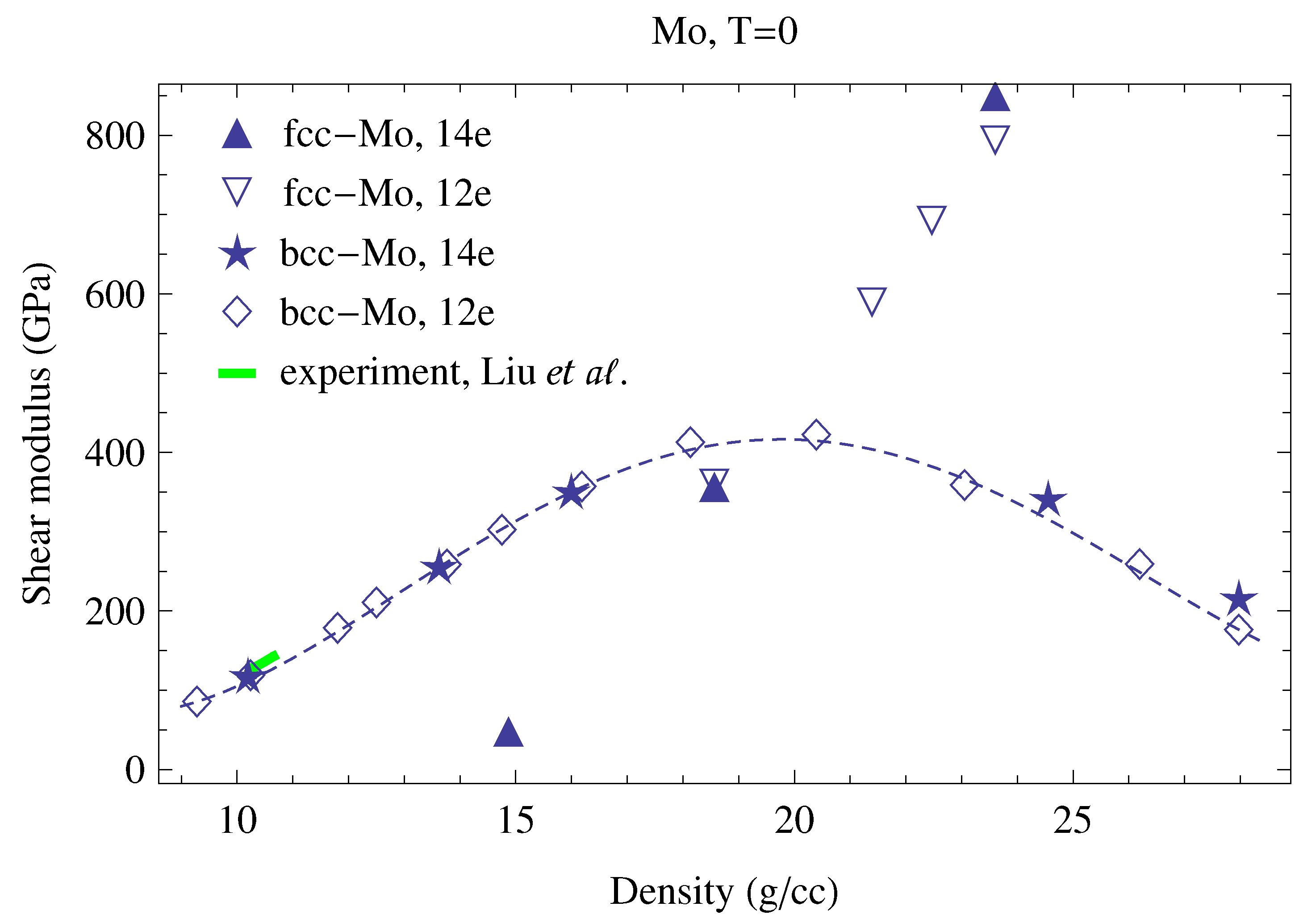
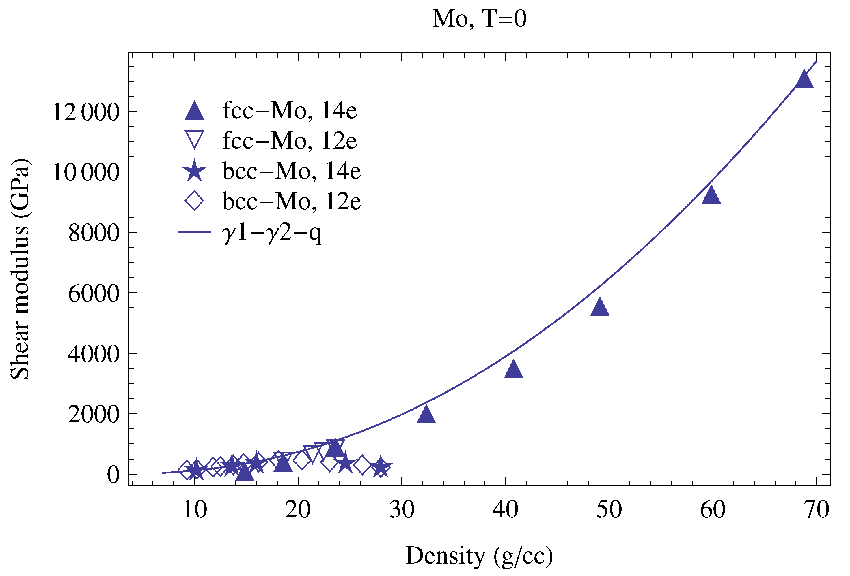
5.1. Cold Shear Modulus of bcc-Mo and fcc-Mo from VASP

In the following we present the results of our calculations of the T = 0 shear moduli of both bcc-Mo and fcc-Mo, as well as the finite-T shear modulus of bcc-Mo using the DFT code VASP (Vienna Ab initio Simulation Package). We use the generalized gradient approximation (GGA) with the Perdew-Burke-Ernzerhof (PBE) exchange-correlation functional. We model Mo using two core-valence representations, namely [ 30 Zn ] 4 p 6 4 d 5 5 s 1 and [ 18 Ar 3 d 10 ] 4 s 2 4 p 6 4 d 5 5 s 1 , i.e., we assign, respectively, the 12 or 14 outermost electrons of Mo to the valence. The valence electrons are represented with a plane-wave basis set with a cutoff energy of 400 eV for the 12-electron representation, and 550 eV for the 14-electron one, while the core electrons are represented by projector augmented-wave (PAW) pseudopotentials. The core radii (the largest values of RCUTs among those for each of the quantum orbitals) of the two pseudopotentials are, respectively, 2.5 a.u., or 1.323 Å and 2.3 a.u., or 1.217 Å. Numerical errors in the calculations using VASP will remain almost negligible until the nearest neighbor distance reaches 2 × RCUT / ( 1.25 ± 0.05 ) [41]. Hence, with these pseudopotentials, one can study systems with densities up to ∼35 g/cm 3 and ∼45 g/cm 3 . At higher densities one should expect the overlap of interatomic spheres starting to develop. But since this overlap is generally allowed and handled well by VASP, in contrast to some other electronic structure codes that give huge errors when the atomic spheres overlap considerably [41], numerical errors in the VASP calculations should remain small at densities much higher than the above two values, specifically at T = 0 when atoms remain in the equilibrium positions. Hence, we expect our calculations of the cold elastic constants to be fairly accurate to the highest density considered.
We used a 5 × 5 × 5 (250-atom) supercell for bcc-Mo and a 4 × 4 × 4 (256-atom) supercell for fcc-Mo with a 5 × 5 × 5 k-point mesh in both cases. Full energy convergence (to ≲0.5 meV/atom) was checked in each simulation. We followed the scheme for the calculation of the shear modulus suggested by Hill, namely, averaging the Voigt ( V ) and Reuss ( R ) upper and lower bounds on the isotropic shear modulus, which for a cubic system are
G V = 2 C + 3 C 44 5 , G R = 5 2 C + 3 C 44 1 .
The Voigt-Reuss-Hill average shear modulus obtained in this way is
G V R H = G V + G R 2 = 3 C 2 + 3 C 44 2 + 19 C C 44 15 C + 10 C 44 .
Here C ( C 11 C 12 ) / 2 and C 44 are the single-crystal elastic constants. A methodology for calculating C and C 44 was developed by Söderlind et al. [42]. To evaluate C , the cubic lattice is deformed by the (volume conserving) transformation
1 + δ 0 0 0 1 + δ 0 0 0 1 ( 1 + δ ) 2 .
The resulting energy change is
Δ E V eq = 6 C δ 2 + O ( δ 3 ) ,
where V eq is the equilibrium volume of the system. Similarly, C 44 is obtained by applying the (volume conserving) transformation
1 δ 0 δ 1 0 0 0 1 1 δ 2 ,
resulting in an energy change
Δ E V eq = 2 C 44 δ 2 + O ( δ 4 ) .
In our calculations, we have evaluated the energy as a function of δ at intervals of 0.01 up to δ = 0.05 for the C 44 case. For the C case, the energy is not an even function of δ , and so negative values of δ were used as well ( 0.03 δ 0.03 ) . The resulting E ( δ ) were fit to third- and fourth-degree polynomials for C and C 44 , respectively, and the quadratic coefficient was used to evaluate the elastic constant from Equation (38) or Equation (39).
In Figure 5 our multi-phase analytic model for G ( ρ , 0 ) is compared with our ab initio results for bcc-Mo and fcc-Mo.

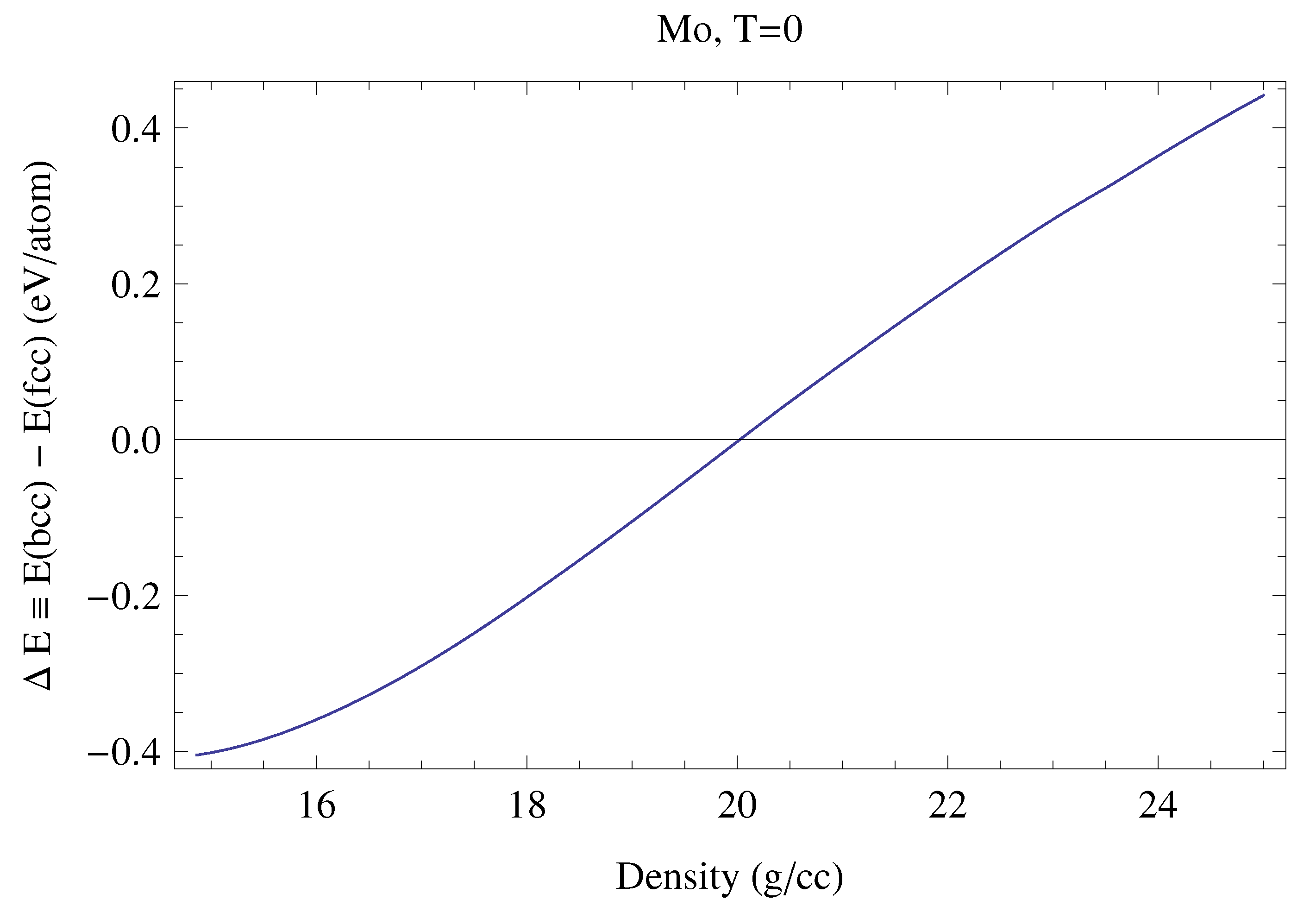
5.2. bcc-fcc Phase Transition in Mo

Figure 4 and Figure 5 show that with increasing density the cold shear modulus of bcc-Mo first increases but then decreases and eventually turns negative at ρ 30 g/cm 3 . This behavior is due to a dynamic instablity which sets in at ∼20 g/cm 3 ( V 8 Å 3 /atom, or P 700 GPa), and which is confirmed by the DFT-based phonon spectra shown in Figure 1. At the same time, at T = 0 fcc-Mo dynamically stabilizes at ∼14.5 g/cm 3 ( P 200 GPa). The T = 0 free energy calculations demonstrate that fcc-Mo becomes thermodynamically more stable than bcc-Mo at ρ 20 g/cm 3 ( P 700 GPa); see Figure 6. The accurate calculation of the two enthalpies gives the following bcc-fcc transition parameters:
P bcc fcc = 680.0 GPa , ρ ( bcc ) bcc fcc = 20.033 g / cm 3 , ρ ( fcc ) bcc fcc = 20.404 g / cm 3 ,
that is, a volume change of ∼2%. At lower P fcc-Mo dynamically stabilizes at nonzero T (the P-T stability regions of fcc-Mo are discussed in [17]) but, as we noted above, full free energy calculations rule out the possibility of fcc-Mo being thermodynamically more stable than bcc-Mo below 700 GPa.

5.3. Melting Curve of Mo

Figure 7 compares our generalized melt-shear model for Mo to the available theoretical data on the melting of Mo [34,43,44], including our own ab initio QMD result for the melting temperature of fcc-Mo at a density of 23.6 g/cm 3 . Our simulations were carried out using the Z method implemented with VASP which is described in detail in Reference [45]. We used a 500-atom ( 5 × 5 × 5 ) fcc-Mo supercell. The simulations were carried out with a single Γ -point (full energy convergence, to ≲1 meV/atom, was achieved with such a large supercell), having 14 electrons of Mo in the valence. We chose to generate a melting datapoint for fcc-Mo to check that the unified model describes this phase as well as it describes bcc-Mo on which the model is based. Since bcc-Mo is dynamically unstable at a density of 23.6 g/cm 3 (a pressure of ∼1300 GPa), it is reasonable to assume that Mo melts from fcc at this density.
We carried out seventeen QMD runs on fcc-Mo at ρ = 23.6 g/cm 3 (a lattice constant of 3.0 Å) with initial temperatures from 42,500 K to 47,500 K separated by an increment of 312.5 K. Figure 8 and Figure 9 illustrate the time evolution of T and P in three of these seventeen QMD runs, with initial Ts of 44,687.5, 45,000, and 45,312.5 K. The 45,000 K run is the melting run [45] for which ( P m , T m ) ( 1300 GPa , 18 , 500 K ) .
As Figure 7 clearly demonstrates, the analytic melting curve of our unified model is in excellent agreement with all the theoretical data on bcc-Mo, including our QMD datapoint on fcc-Mo.

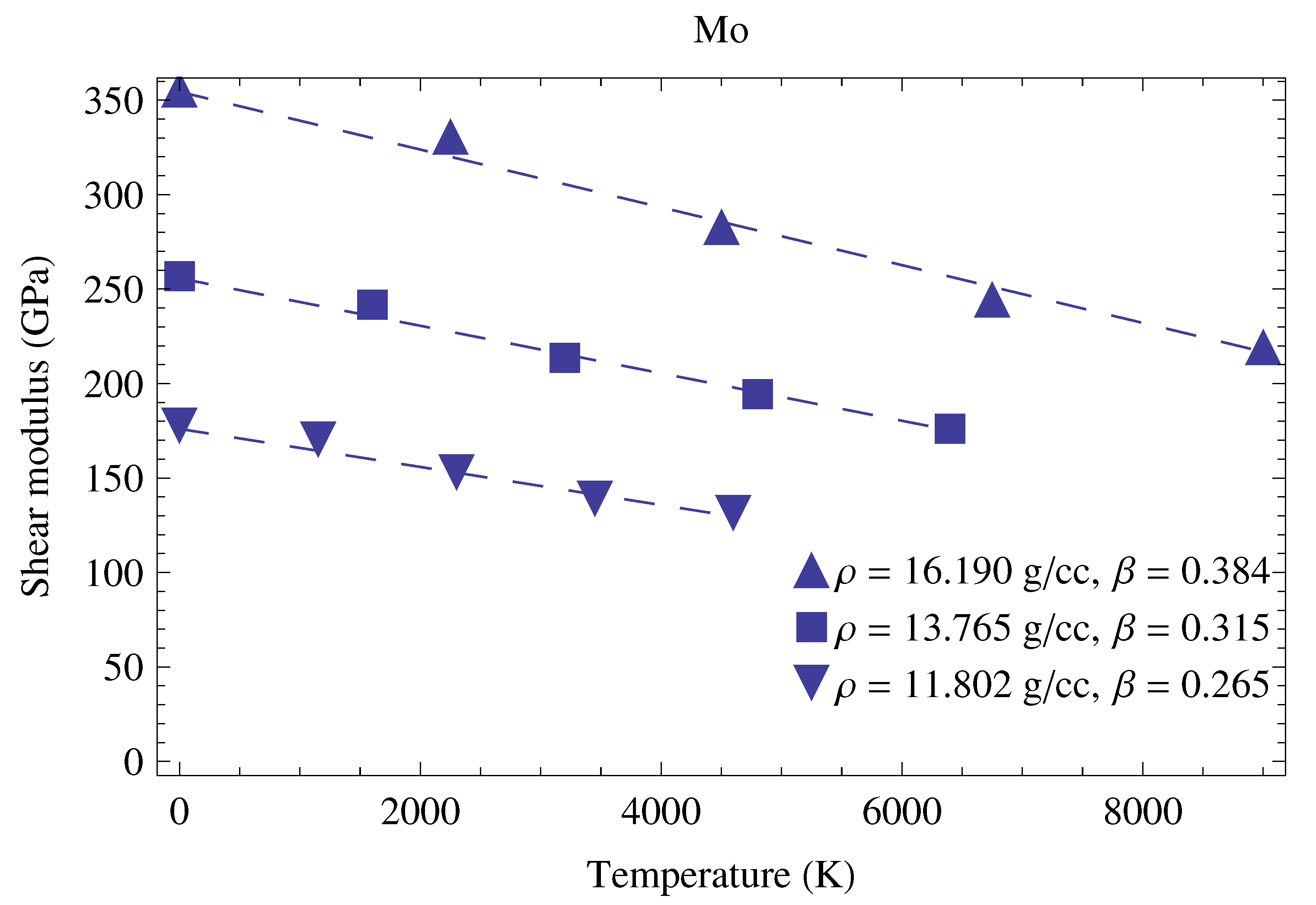
5.4. Thermoelastic Softening Parameter

In the Preston-Wallace (PW) thermoelasticity model [6] the thermoelastic softening parameter β can in principle be a function of density, so the most general analytic form of the PW model is
G ( ρ , T ) = G ( ρ , 0 ) 1 β T T m ( ρ ) ,
instead of Equation (4). It was determined in [6] that for Mo at P = 0 , β = 0.23 . In order to ascertain if there is any density dependence of β , we carried out QMD simulations of elastic constants at a set of four nonzero Ts, specifically, ∼ T m / 4 , T m / 2 , 3 T m / 4 and T m , at three different densities. The slope of a straight line fitted to the four nonzero T values combined with the T = 0 value calculated earlier gives the value of β at the corresponding density. We followed the same strategy as for the T = 0 simulations described above. We employed a Nosé-Hoover thermostat and used the Nosé algorithm with controlled temperature oscillations around the initial T so that their frequency is the same as the characteristic phonon frequency of the atomic system at the P-T conditions of the QMD run. The finite-T simulations typically require between 5000 and 10,000 time steps of 1 fs to achieve full energy convergence and to produce sufficiently long output for the extraction of reliable averages for the values of energy that are used in Equations (38) and (39) to calculate the corresponding values of the elastic constants.
Our QMD simulations of G as a function of T at three different densities, shown in Figure 10, demonstrate that, at least for bcc-Mo, β does depend on density. The best fit to the three datapoints subject to the constraint that β ( ρ = 10.25 ) = 0.23 ( ρ in g/cm 3 ) is
β = β ( ρ ) = 0.23 + 0.0212 ( ρ 10.25 ) 1.11 .

6. Thermoelasticity Model of Molybdenum

The unified analytic melt-shear model for a multi-phase material developed in this paper gives the cold shear modulus and melting temperature at all densities across all solid phases. For example, in Figure 5 the model curve covers bcc-Mo at densities up to ∼20 g/cc and smoothly transitions to fcc-Mo at higher ρ . In order to have a model of the thermoelasticity of any given solid phase of a multi-phase material, the corresponding unified model must be supplemented with the information on (i) the density interval in which the solid phase is dynamically stable; and (ii) the density dependence of the thermoelastic softening parameter over this density interval. In the following, we consider bcc-Mo as an example of such a complete thermoelasticity model.
Equation (41) with G ( ρ , 0 ) and T m ( ρ ) given by Equations (13) and (14), respectively, and β ( ρ ) as in Equation (42) define the complete thermoelasticity model of bcc-Mo over the range of densities in which it is dynamically stable. To illustrate its fidelity, we now consider shear modulus along the principal Hugoniot of Mo. This is one of the applications of our model that can be directly compared to experiment.

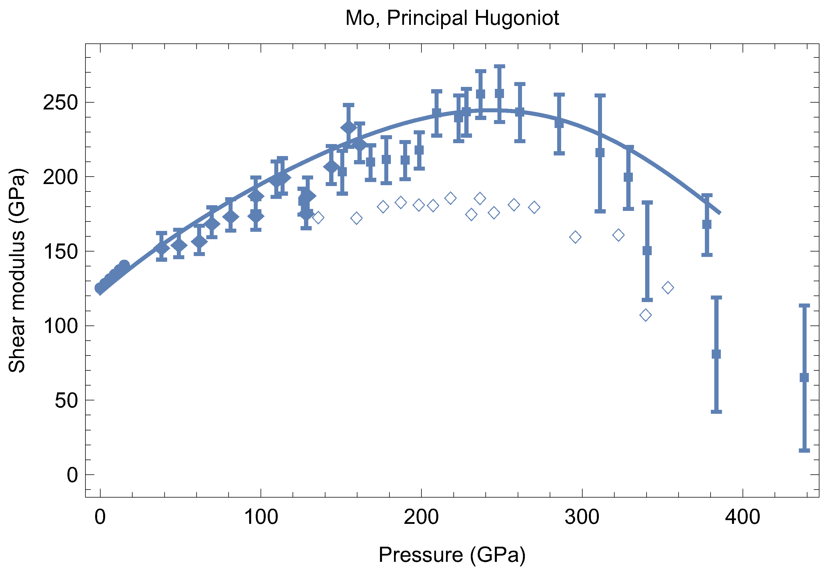
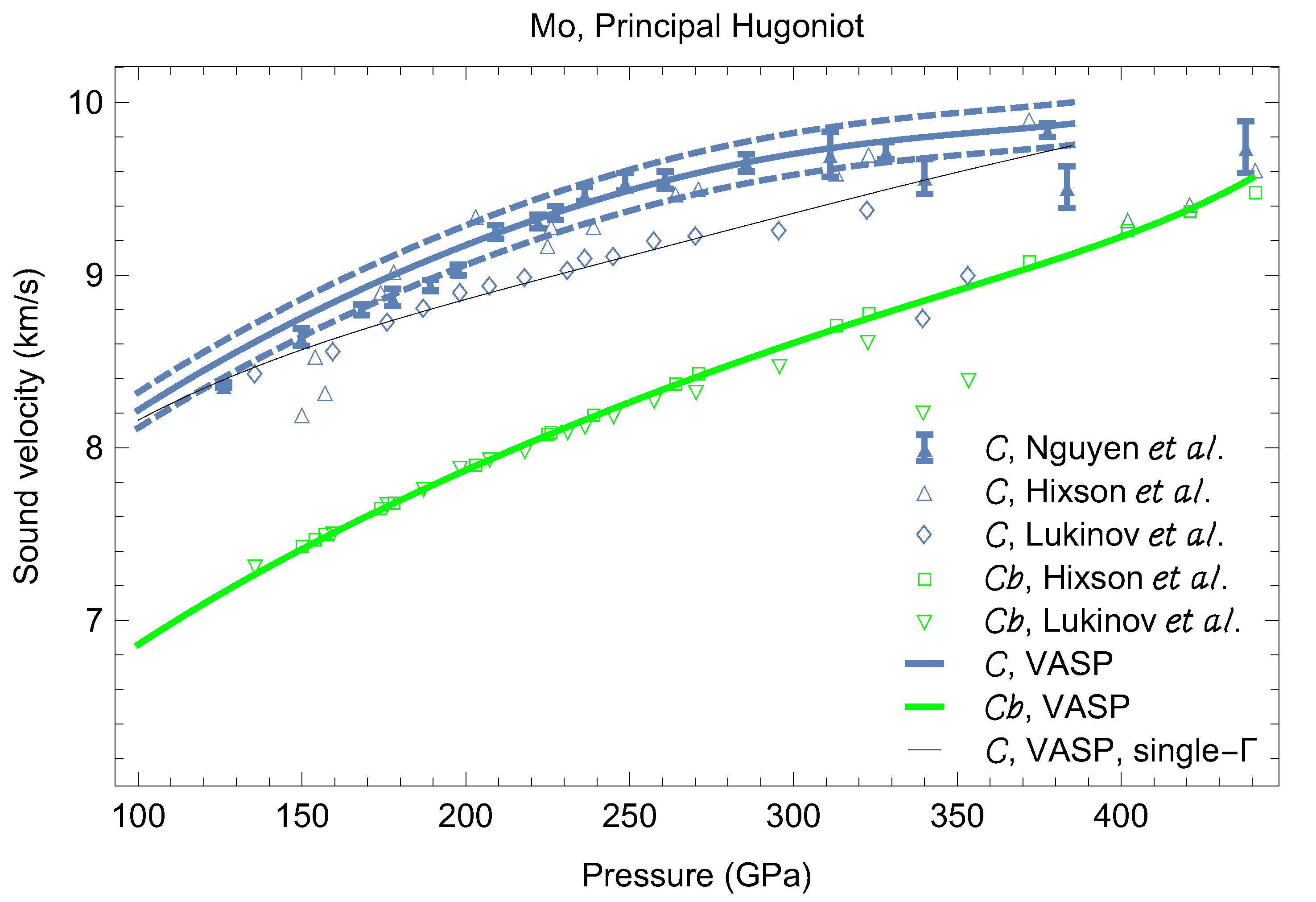
Shear Modulus and Sound Velocities Along the Principal Hugoniot

Using the cold G from Equation (31) in the PW elasticity model, along with (i) T m ( ρ ) from the new analytic model; (ii) β = β ( ρ ) from Equation (42); and (iii) the temperature along the Hugoniot gives the shear modulus along the Hugoniot.
We found two different sources of data on T ( ρ ) along the Hugoniot: [46,47]. The best fits to the two sets of data are, respectively,
T ( ρ ) = 293 + 58.98 ( ρ 10.206 ) 2.78586 ,
and
T ( ρ ) = 293 + 52.2891 ( ρ 10.215 ) 2.87282 .
The intersection of the melting curve (14) with the parameter values from (35) with either of the above T ( ρ ) along the Hugoniot predicts the corresponding Hugoniot melting point, and it turns out to be ( ρ , T ) = ( 16.19 , 8900 ) and ( 16.10 , 8800 ) , respectively, in good agreement with the theoretical estimate ( 16.5 , 9300 ) by Hixson et al. [7] based on their experimental results. Here we take Equation (43) as that for T ( ρ ) along the principal Hugoniot of Mo.
We use the experimental P ( ρ ) (those of [46,47] are virtually identical) to calculate G as a function of pressure along the bcc-Mo Hugoniot; our results are shown in Figure 2 and are in good agreement with experiment. The experimental data are consistent with bcc-Mo along the entire Hugoniot; there is no evidence for any other crystal structure such as Phase II [24]. Our G = G ( P ) model curve can be approximated by
G ( P ) = 122.0 + 0.94 P 3.0 × 10 3 P 2 + 1.2 × 10 5 P 3 2.8 × 10 8 P 4 2.4 × 10 11 P 5 + 8.3 × 10 14 P 6 .
We also calculated sound velocities C L and C B along the Hugoniot; they are shown in Figure 3. We used B = ρ d P / d ρ calculated from the experimental P ( ρ ) .
Our results on the shear modulus and sound velocities in bcc-Mo along its principal Hugoniot are compared to experimental data in Figure 2 and Figure 3. The shear modulus of bcc-Mo increases with P up to ∼240 GPa but then decreases. This P dependence is not due to a high-P phase such as Phase II proposed by Errandonea et al. [24] for its explanation but is rather a property of bcc-Mo.
In Appendix B we consider two additional examples of transition metals with ambient bcc structure that dynamically destabilizes with increasing pressure, namely, tantalum and tungsten. We find the same behavior of G along their Hugoniots as that of Mo. These two additional examples strongly suggest that this behavior may be typical for transition metals with ambient bcc structure that becomes dynamically unstable at higher P. The parameters for the thermoelasticity models of Mo, Ta, and W are given in Table 1.

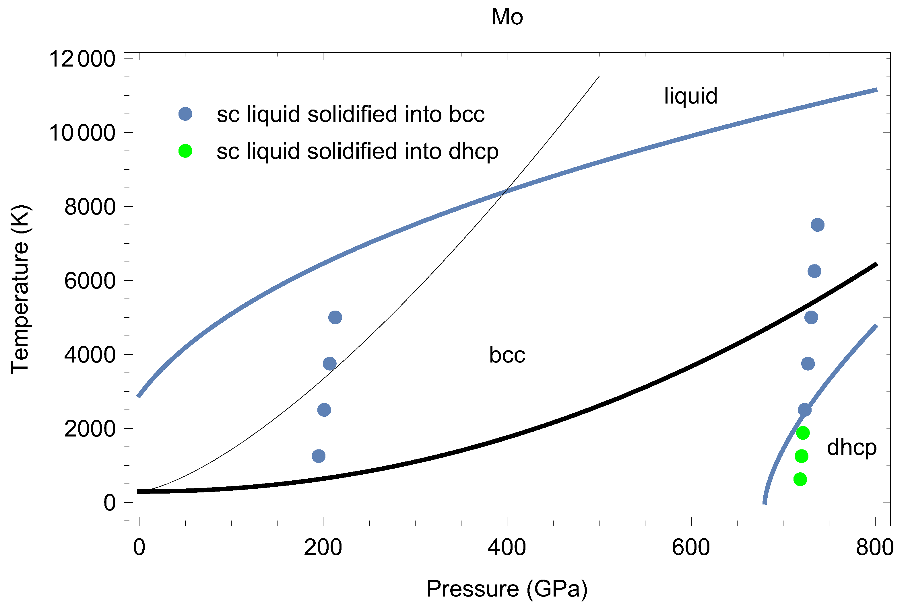
7. The Phase Diagram of Molybdenum

The results obtained in this work suggest that the phase diagram of Mo cannot be extended beyond Figure 1 of Reference [11]. Indeed, if there are other solid phase fields on the phase diagram of Mo, in addition to bcc which is well established experimentally, and perhaps some other solid structure (fcc, hcp, dhcp, etc.) which is so far only predicted theoretically, neither Hugoniot nor ramp-wave compression curves cross into them. Hence, further refinement of the phase diagram of Mo is not yet feasible. However, we have confirmed that the topology of the phase diagram of Mo is essentially the same as in Figure 1 of Reference [11] and is represented in Figure 11. To this end, we carried out two sets of independent inverse Z runs [48] to solidify liquid Mo and to check whether there is any solid-solid phase boundary so that liquid Mo solidifies into bcc on one side of this boundary and into another solid structure on the other side. We used a computational cell of 512 atoms prepared by melting a 8 × 8 × 8 solid simple cubic (sc) supercell which would eliminate any bias towards solidification into bcc or any other solid structure (fcc, hcp, dhcp, etc.). We used sc unit cells of 2.225 and 1.985 Å; the dimensions of bcc unit cells having the same volume as the sc ones are 2.80 and 2.50 Å, respectively, which corresponds to ∼200 and 700 GPa.
We carried out N V T simulations using the Nosé-Hoover thermostat with a timestep of 1 fs. Complete solidification typically required from 15 to 25 ps, or 15,000–25,000 timesteps. The inverse Z runs indicate that liquid Mo only solidifies into bcc at ∼200 GPa in the whole temperature range from 0 to essentially the corresponding T m . However, at ∼700 GPa it solidifies into bcc above the transition boundary in Figure 11, while below this boundary it solidifies into another solid structure. The radial distribution functions (RDFs) of the final solid states are noisy; upon fast quenching of the three structures to low T , where RDFs are more discriminating, and by comparing them to the RDFs of fcc, hcp and dhcp, we conclude that dhcp is the closest strucure to those that liquid Mo solidies into below the transition boundary.
The RDFs of the solidified states at ∼700 GPa above the transition boundary are shown in Figure 12, and of those solidified below the transition boundary in Figure 13. The 2500 K state virtually lies on the boundary. We tentatively assign it to bcc, because it definitely has features of bcc (RDF peaks at R 55 , 65 and 90, small peak at R 80 , etc.). At the same time it certainly has some features that are both uncharacteristic of bcc (e.g., the disappearance of the bcc split-peak at R 40 ) and characteristic of dhcp (a small peak at R 50 , etc.). The RDF of this 2500 K state is shown in Figure 13 also, for comparison to other dhcp states, including the real dhcp-Mo (at 2500 K). Most likely, this 2500 K state is a mixture of both bcc and dhcp.
A few more comments are in order. The 8750 K state at ∼700 GPa did not solidify, most likely for the reason of not being supercooled enough to intiate the solidification process [48]. Indeed, 8750 K constitutes ∼0.8 of the corresponding T m (20% of supercooling) while for the other set of points at ∼200 GPa, the highest solidification T of 5000 K constitutes ∼0.75 of the corresponding T m (25% of supercooling) which apparently allows for the solidification process to go through in this case. The 625 K state at ∼700 GPa is amorphous, with a characteristic RDF shoulder at R 60–70, for the reason of the corresponding solidification T being too low, most likely below the corresponding T of vitrification.

8. Concluding Remarks

We have generalized the unified analytic melt-shear model that we introduced a decade ago to multi-phase materials. We have described a new scheme for calculating the values of the model parameters for both G and T m at all densities. The new model was applied to molybdenum, a multi-phase material having body-centered cubic (bcc) structure at low ρ and face-centered cubic (fcc) structure at high ρ . The new model was compared to (i) our ab initio results on the T = 0 shear modulus of both bcc-Mo and fcc-Mo as a function of ρ ; and (ii) the available theoretical results on the melting of bcc-Mo and our own quantum molecular dynamics simulations of one high-P melting point of fcc-Mo.
We have constructed a model for G ( ρ , T ) of bcc-Mo at all ρ for which bcc-Mo remains dynamically stable, and all T from 0 to T m . The model is described by Equation (41) in which G ( ρ , 0 ) and β ( ρ ) are given by Equations (31) and (42), respectively, and T m ( ρ ) is given by Equation (14) with γ 1 = 2.1145 and γ 3 and q 3 from Equation (35). We then applied this thermoelasticity model to the calculation of the shear modulus of bcc-Mo along its principal Hugoniot. Our results were compared to experimental data and showed that G of bcc-Mo increases with P up to ∼240 GPa but then decreases. We emphasize that this P dependence is not due to a high-P phase such as Phase II proposed by Errandonea et al. [24] for its explanation. Similar behavior of G along the Hugoniot is also found in the transition metals Ta and W, thereby suggesting that it may be typical for transition metals with ambient bcc structure that become dynamically unstable at higher P . Thus, we agree with the common conclusion of a number of recent papers [8,9,26] that no s-s phase transition can be definitively inferred from the sound velocity data on Mo. If there are other solid phase fields on the phase diagram of Mo, in addition to bcc, neither Hugoniot nor ramp-wave compression curves cross into them. In the absence of additional experimental and/or theoretical information on other solid phases, our current knowledge of the phase diagram of Mo cannot be extended beyond Figure 1 of Reference [11].
Finally, our thermoelasticity model for bcc-Mo predicts a decrease in G with P on the principal Hugoniot at pressures above ∼204 GPa, hence the decrease in G with P is not evidence for a s-s transition on the Hugoniot.

Author Contributions

The authors contributed equally to this work.

Funding

This research received no external funding.

Acknowledgments

The work was done under the auspices of the US DOE/NNSA. The QMD simulations were performed on the LANL clusters Pinto and Moonlight as parts of the Institutional Computing projects w17_thermoelasticity, w17_molybdenum, and w18_meltshear.

Conflicts of Interest

The authors declare no conflict of interest.

Appendix A. Is There a Solid-Solid Transition on the Mo Hugoniot?

Sound velocities along the Mo principal Hugoniot have been measured (to the best of our knowledge) in just three sets of experiments: Hixson et al. in 1989 [7], Nguyen et al. in 2014 [8], and Zhang et al. in 2015 [26]. The data of Hixson et al. show two discontinuities in the longitudinal sound velocity, C L , at pressures of 210 GPa ( T 4100 K) and 390 GPa ( T 10,000 K). The first discontinuity was attributed to a s-s phase transition (bcc-hcp was suggested in [7]), and the second one to melting. Subsequent studies confirmed melting on the Hugoniot at ∼390 GPa [8,9]. However, Nguyen et al. [8] claimed that a careful statistical analysis of their shock data excludes a discontinuity in C L at ∼200 GPa, that is, their experiments do not indicate a s-s transition along the principal Hugoniot in Mo, nor was it confirmed in subsequent studies [9,26]. Errandonea et al. [24] converted the sound velocity data of References [8,26] into the shear modulus along the Hugoniot using the formula C L 2 = ( B + 4 3 G ) / ρ , where B is the bulk modulus, and concluded that the P dependence of G, specifically a decrease in G with increasing P, is indicative of a transformation of bcc-Mo into another phase, which they called Phase II, at 210–240 GPa.
A presumed s-s phase transition on the Mo Hugoniot has also been a subject of theoretical studies. Using the DFT approach with VASP and employing the quasi-harmonic approximation, Belonoshko et al. [12] determined the high-T bcc-fcc transition boundary at megabar pressures which is consistent with Hixson’s first discontinuity at 210 GPa and ∼4100 K. This result was subsequently challenged by Cazorla et al. [49] who claimed that the stability of other solid phases of Mo is affected by taking into account anharmonicity; specifically, bcc-Mo remains thermodynamically more stable than fcc-Mo if the corresponding anharmonic free energies are used. This conclusion was further corraborated by Zeng et al. [17] who also disprove the high-T bcc-fcc transition at megabar pressures based on the corresponding full (anharmonic) free energies. A careful experimental study of the structure of Mo along the Hugoniot using X-ray diffraction [9] found no solid structure other than bcc.
Despite the results of [17,49] that preclude the high-T s-s phase transition in Mo (at least, the bcc-fcc one) on the Hugoniot, a more recent calculation of C L in bcc-Mo along the Hugoniot by Lukinov et al. [16] revives this idea. Since their results for bcc-Mo disagree with experiment they conclude that the experimental results are evidence for another solid phase of Mo. A detailed discussion of their work goes beyond the scope of this paper. We will, however, focus on three points which imply that the conclusion drawn by the authors of [16] may be incorrect.
1. Lukinov et al. calculate C L along the Hugoniot in bcc-Mo and find out that their theoretical results diverge from experiment above ∼200 GPa and this divergence is beyond experimental error bars. They conclude that the high-P C L data are for another solid phase, hence there is a s-s phase transition on the Hugoniot at ∼200 GPa, in agreement with [7]. They find that C L in the high-P solid phase of Mo is larger than that in bcc. However, an increase in C L across a s-s transition is a very exotic case: the emerging solid phase must be less dense or have smaller elastic constants, or both. No such cases have ever been observed in experiment. In a more realistic scenario, bcc-Mo would convert to either fcc or hcp, one of the two candidates mainly discussed in the literature, and in such a case its C L would go down across the s-s transition; see, e.g., Figure 3 of Reference [50] which shows that C L in fcc-Mo is considerably smaller than that in bcc-Mo.
2. The Hugoniot of another solid phase will have a slope different from that of bcc-Mo and will cross the melting curve at P different from ∼400 GPa. A calculation shows that the Hugoniot of fcc-Mo has a smaller slope than that of bcc-Mo and crosses the Mo melting curve at ∼450 GPa [50]. In fact, the fcc segment of the Mo Hugoniot would have to cross the fcc-Mo melting curve rather than the bcc-Mo one. If fcc-Mo were the physical phase of Mo, its melting curve would be higher than that of bcc-Mo, hence its Hugoniot crossing point would be at even higher pressure, likely ∼500 GPa. The undeniable experimental evidence that melting on the Mo Hugoniot occurs at 380–390 GPa is a serious argument against melting from any solid phase other than bcc.
3. The equation of state (EOS) along the Hugoniot calculated by Lukinov et al., Figure 1 of [16], agrees with experiment over the entire pressure range considered in [16]. Hence, both experiment and theory describe the same solid structure of Mo, namely, bcc-Mo. The reason for the theoretical sound velocity to diverge from experiment may be insufficient accuracy of the calculated elastic constants. Our own tests reveal that for a 250-atom supercell with a single Γ point, as in [16], energy is converged to ≲10 meV/atom (the corresponding 0.01 meV/atom in [16] must be a typo), which is good enough to produce a reliable EOS but not good enough to generate accurate elastic constants. Specifically, in our VASP runs with a single Γ point both the cold elastic constants C ( C 11 C 12 ) / 2 and C 44 , as functions of P , behave normally up to ∼50 GPa where they start softening, stay below the corresponding fully converged C ( P ) and C 44 ( P ) trajectories at ∼100–400 GPa, then start hardening and going back to the fully converged trajectories into which they finally merge at ∼450 GPa. Here the fully converged trajectory is the one with a k-point mesh of 3 × 3 × 3 or any denser. Hence, in the P interval 100–400 GPa the values of both C and C 44 obtained with a single Γ point are too low, and so is G . At the same time, P is fully converged, already with a single Γ point, and so is B ρ d P / d ρ , so that the EOS is accurate. The softening of both C and C 44 pertains at finite T , as our own calculations also demonstrate. Hence, in the pressure interval considered in [16] the elastic constants are such that C and C 44 are too small, and therefore both G and C L are too small also. Figure 2 and Figure 3 clearly demonstrate this point. All the experimental data (except the three lower-P points by Hixson et al.) on Figure 3 are within the 3 σ -wide confidence interval around our theoretical model curve, while the results by Lukinov et al. are outside of this interval. Specifically, with C and C 44 obtained with a single Γ point, Equation (45) is replaced with G ( P ) = 122.0 + 0.94 P 7.3 × 10 4 P 2 3.7 × 10 5 P 3 + 1.6 × 10 7 P 4 2.3 × 10 10 P 5 + 7.3 × 10 14 P 6 . The corresponding C L = ( B + 4 / 3 G ) / ρ is shown in Figure 3 as a thin black line; this line covers all the data points from Reference [16] except for the last 3 points that are very close to T m . One sees clearly that the single- Γ C L stays below the corresponding fully converged C L at ∼100–400 GPa, consistent with a similar behavior of G . Thus, we believe we have found the explanation for the numerical results of Reference [16] being in disagreement with experiment.
At the same time, B and the bulk sound velocity C B = B / ρ are quite accurate, as clearly seen in Figure 3: the results of [16] on C B are in good agreement with experiment (except for the last 3 points).
In summary, the assertion of Lukinov et al. that there is a solid-solid transition on the Mo Hugoniot is very likely incorrect.

Appendix B. Unified Analytic Melt-Shear Models for Ta and W

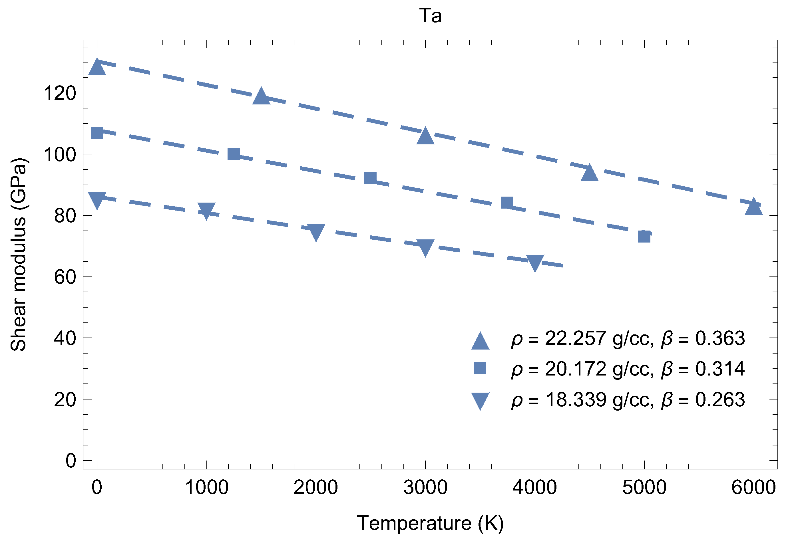
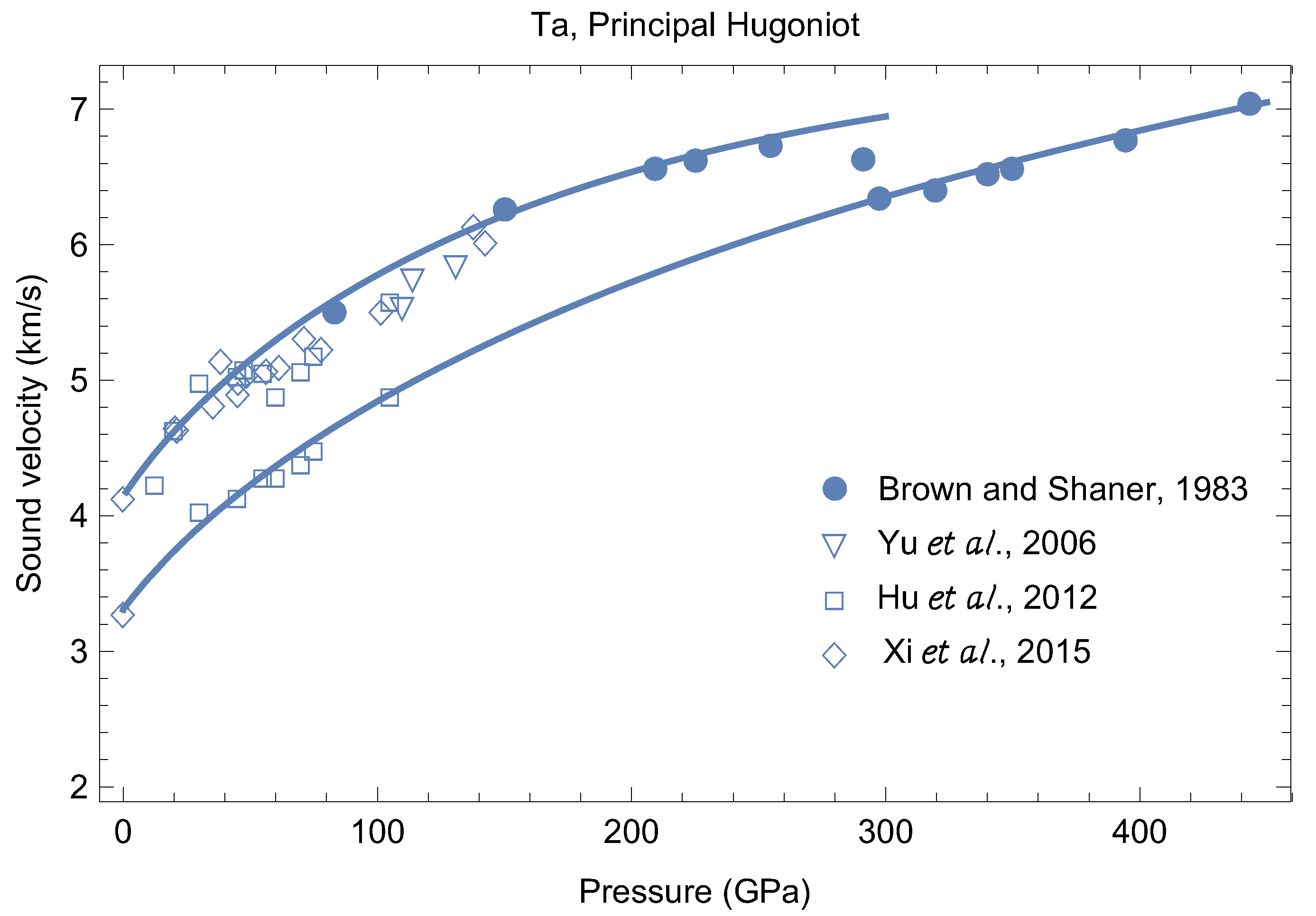
Appendix B.1. Tantalum

At ambient conditions Ta is, like Mo, a bcc material. Experiments show that it is structurally stable to a pressure of a third of a terapascal [51,52]. However, with increasing P, Ta is predicted to convert into another solid phase. It is argued in References [53,54] that a transition from bcc to one of the hexagonal structures among those with different stackings of atomic layers (e.g., hexagonal close-packed (hcp), face-centered cubic (fcc), double-hcp (dhcp), etc.), or even a mixture of those stackings, is expected to occur at ultrahigh pressures. Since fcc-Ta becomes dynamically stable with increasing P [55], in addition to being thermodynamically more stable than bcc-Ta, fcc-Ta is a good candidate for the high-P solid structure of Ta.
The unified analytic melt-shear model for Ta that covers bcc-Ta at lower P and another solid phase (e.g., fcc-Ta) at higher P can be constructed following the same procedure that we used above for Mo. Here we skip the technical details for the sake of brevity. The values of the Ta model parameters are shown in Table 1 in the main text.
Our QMD simulations of G for Ta as a funtion of T , at three different densities, shown in Figure A1 demonstrate that, at least for bcc-Ta, β depends on density, and this dependence is given by ( ρ in g/cm 3 )
β = β ( ρ ) = 0.23 + 0.021 ( ρ 16 . 74 ) 1.09 ,
which is very similar to the corresponding β ( ρ ) for Mo.
The longitudinal and bulk sound velocities in bcc-Ta along its principal Hugoniot are shown in Figure A2 along with the corresponding experimental data from [56,57,58,59].
Figure A1. The shear modulus of bcc-Ta as a function of T at three different densities.
Crystals 09 00086 g0a1
Figure A2. Longitudinal (upper) and bulk (lower) sound velocities in bcc-Ta along its principal Hugoniot: comparison of the unified analytic melt-shear model (curves) to the experimental data of References [56,57,58,59].
Crystals 09 00086 g0a2

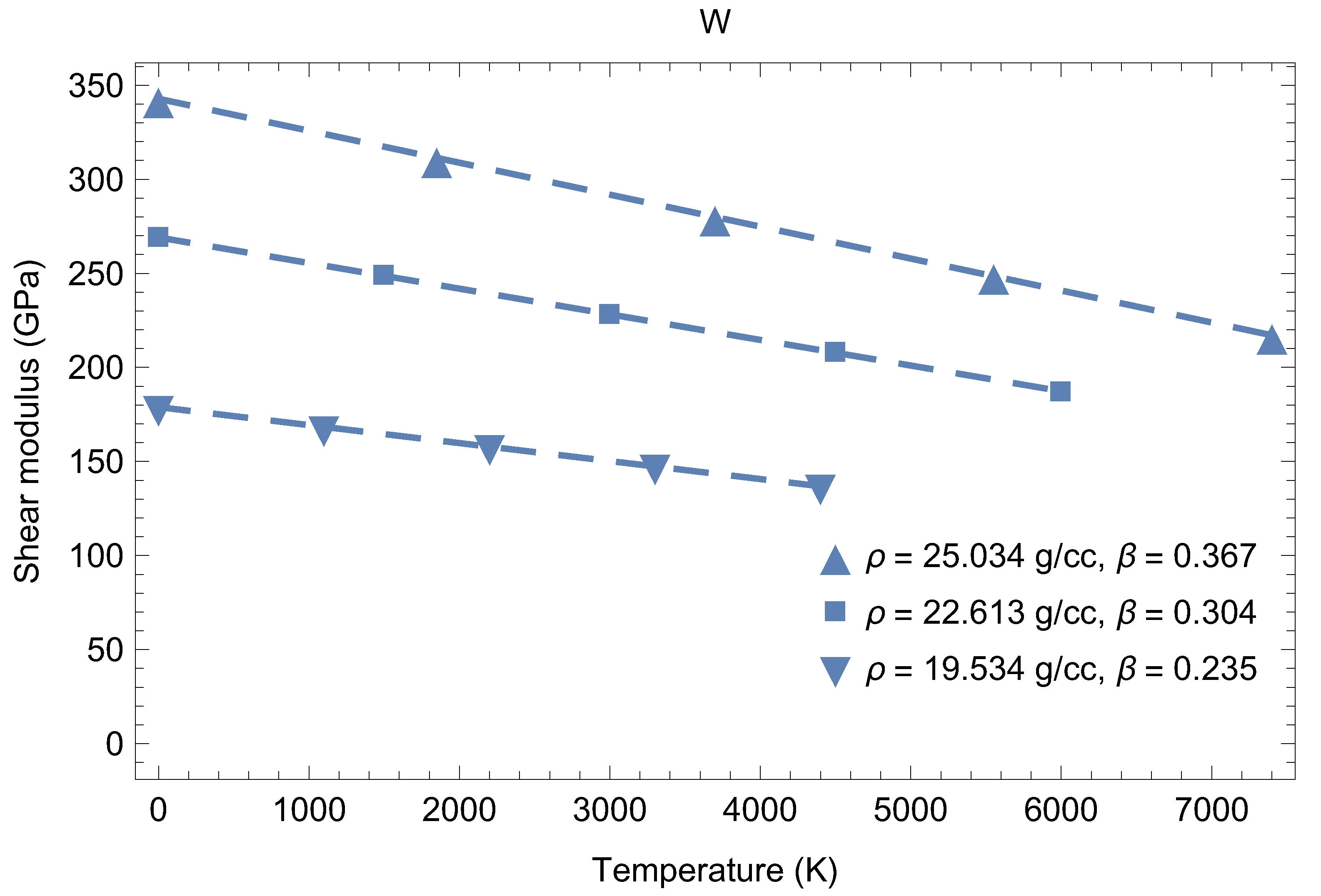
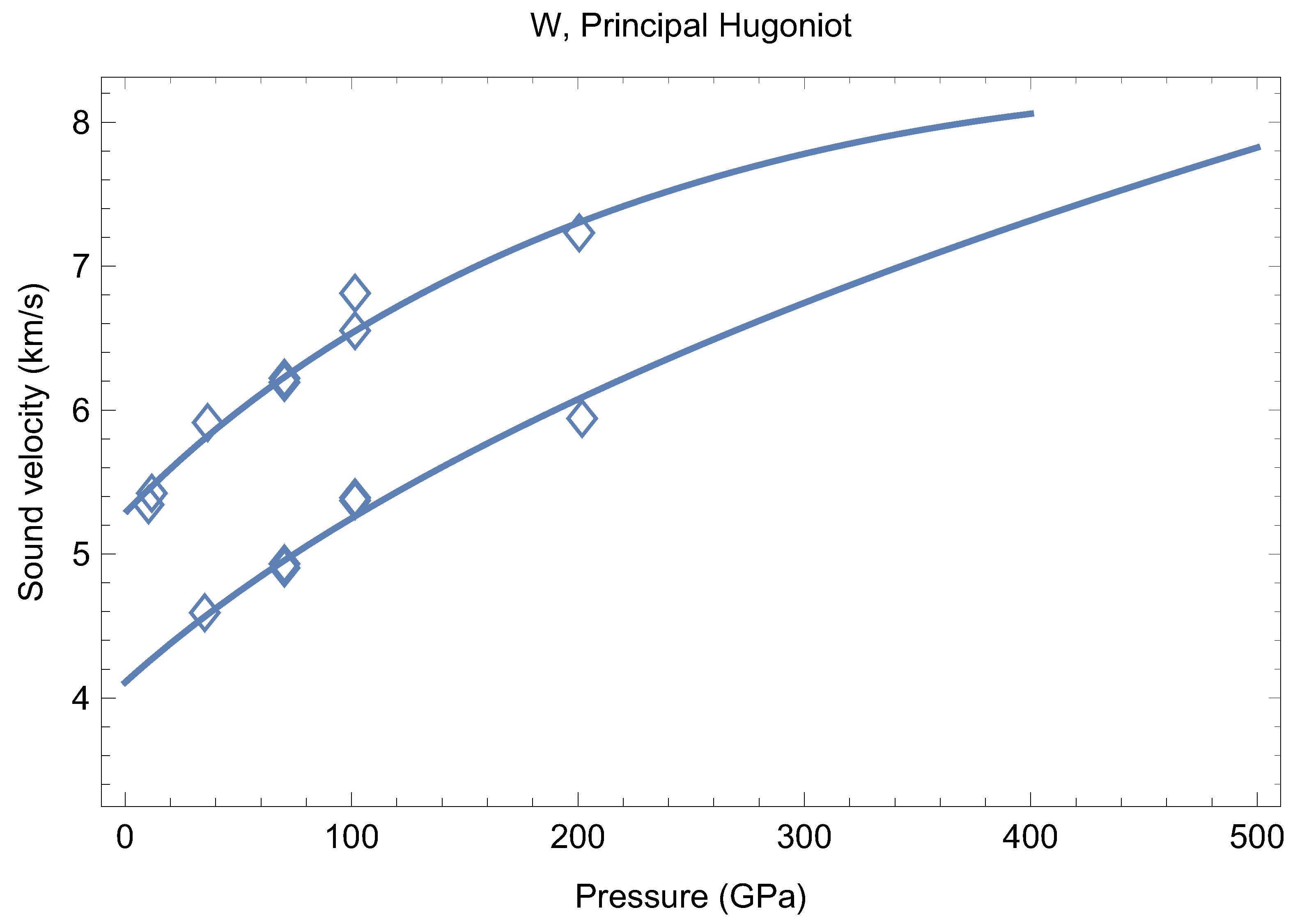
Appendix B.2. Tungsten

Tungsten is our third example of a transition metal with ambient bcc structure. Experiment shows that it is structurally stable to 423 GPa [10]. However, with increasing P , W is also predicted to convert into another solid phase, just like both Mo and Ta. A very recent theoretical study [60] demonstrates that fcc-W becomes dynamically stable at ∼450 GPa while bcc-W becomes dynamically unstable with increasing P ; since fcc-W also becomes thermodynamically more stable than bcc-W [60], fcc-W is a good candidate for the high-P solid structure of W.
We have constructed the unified analytic melt-shear model for W for which the numerical values of the parameters are shown in Table 1 in the main text.
Our QMD simulations of G for W as a function of T , at three different densities, shown in Figure A3, demonstrate that β for bcc-W depends on density ( ρ in g/cm 3 )
β = β ( ρ ) = 0.23 + 0.021 ( ρ 19.31 ) 1.07 .
This is very similar to Equations (42) and (46) for Mo and Ta, respectively.
Figure A3. The shear modulus of bcc-W as a function of T at three different densities.
Crystals 09 00086 g0a3
The longitudinal and bulk sound velocities in bcc-W along its principal Hugoniot are shown in Figure A4 along with the corresponding experimental data from [61].
As clearly seen in Figure A2 and Figure A4, both bcc-Ta and bcc-W exhibit exactly the same behavior as bcc-Mo, namely, the softening of the shear modulus along the principal Hugoniot that shows up as the softening of C L in a shock-wave experiment.
Figure A4. Longitudinal (upper) and bulk (lower) sound velocities in bcc-W along its principal Hugoniot: comparison of the unified analytic melt-shear model (curves) to the experimental data of Reference [61] (diamonds).
Crystals 09 00086 g0a4

References

  1. Burakovsky, L.; Greeff, C.W.; Preston, D.L. Analytic model of the shear modulus at all temperatures and densities. Phys. Rev. B 2003, 67, 094107. [Google Scholar] [CrossRef]
  2. Burakovsky, L.; Preston, D.L. Analytic model of the Grüneisen parameter all densities. J. Phys. Chem. Sol. 2004, 65, 1581. [Google Scholar] [CrossRef]
  3. Young, D.A. Phase Diagrams of the Elements; University of California Press: Berkeley, CA, USA, 1991. [Google Scholar]
  4. Burakovsky, L.; Preston, D.L. Analysis of dislocation mechanism for melting of elements. Solid State Commun. 2000, 115, 341. [Google Scholar] [CrossRef]
  5. Burakovsky, L.; Preston, D.L.; Silbar, R.R. Melting as a dislocation-mediated phase transition. Phys. Rev. B 2000, 61, 15011. [Google Scholar] [CrossRef]
  6. Preston, D.L.; Wallace, D.C. A model of the shear modulus. Solid State Commun. 1992, 81, 277. [Google Scholar] [CrossRef]
  7. Hixson, R.S.; Boness, D.A.; Shaner, J.W.; Moriarty, J.A. Acoustic velocities and phase transitions in molybdenum under strong shock compression. Phys. Rev. Lett. 1989, 62, 637. [Google Scholar] [CrossRef]
  8. Nguyen, J.H.; Akin, M.C.; Chau, R.; Fratanduono, D.E.; Ambrose, W.P.; Fat’yanov, O.V.; Asimow, P.D.; Holmes, N.C. Molybdenum sound velocity and shear modulus softening under shock compression. Phys. Rev. B 2014, 89, 174109. [Google Scholar] [CrossRef]
  9. Wang, J.; Coppari, F.; Smith, R.F.; Eggert, J.H.; Lazicki, A.E.; Fratanduono, D.E.; Rygg, J.R.; Boehly, T.R.; Collins, G.W.; Duffy, T.S. X-ray diffraction of molybdenum under shock compression to 450 GPa. Phys. Rev. B 2015, 92, 174114. [Google Scholar] [CrossRef]
  10. Ruoff, A.L.; Xia, H.; Xia, Q. The effect of a tapered aperture on X-ray diffraction from a sample with a pressure gradient: Studies on three samples with a maximum pressure of 560 GPa. Rev. Sci. Instrum. 1992, 6, 4342–4348. [Google Scholar] [CrossRef]
  11. Wang, J.; Coppari, F.; Smith, R.F.; Eggert, J.H.; Lazicki, A.E.; Fratanduono, D.E.; Rygg, J.R.; Boehly, T.R.; Collins, G.W.; Duffy, T.S. X-ray diffraction of molybdenum under ramp compression to 1 TPa. Phys. Rev. B 2016, 94, 104102. [Google Scholar] [CrossRef]
  12. Belonoshko, A.B.; Burakovsky, L.; Chen, S.P.; Johansson, B.; Mikhaylushkin, A.S.; Preston, D.L.; Simak, S.I.; Swift, D.C. Molybdenum at high pressure and temperature: Melting from another solid phase. Phys. Rev. Lett. 2008, 100, 135701. [Google Scholar] [CrossRef] [PubMed]
  13. Cazorla, C.; Alfè, D.; Gillan, M.J. Comment on “Molybdenum at high pressure and temperature: Melting from another solid phase”. Phys. Rev. Lett. 2008, 101, 049601. [Google Scholar] [CrossRef] [PubMed]
  14. Mikhaylushkin, A.S.; Simak, S.I.; Burakovsky, L.; Chen, S.P.; Johansson, B.; Preston, D.L.; Swift, D.C.; Belonoshko, A.B. Mikhaylushkin et al. Reply. Phys. Rev. Lett. 2008, 101, 049602. [Google Scholar] [CrossRef]
  15. Cai, L.-C.; Zeng, Z.-Y.; Zhang, X.-L.; Hu, J.-B. Experimental research on high pressure phase transitions of Mo and Ta. EPJ Web Conf. 2010, 8, 00028. [Google Scholar] [CrossRef]
  16. Lukinov, T.; Simak, S.I.; Belonoshko, A.B. Sound velocity in shock compressed molybdenum obtained by ab initio molecular dynamics. Phys. Rev. B 2015, 92, 060101. [Google Scholar] [CrossRef]
  17. Zeng, Z.-Y.; Hu, C.-E.; Zhang, W.; Niu, Z.-W.; Cai, L.-C. Dynamical stability of Mo under high pressure and high temperature. J. Appl. Phys. 2014, 116, 133518. [Google Scholar] [CrossRef]
  18. Krasilnikov, O.M.; Belov, M.P.; Lugovskoy, A.V.; Mosyagin, I.Y.; Vekilov, Y.K. Elastic properties, lattice dynamics and structural transitions in molybdenum at high pressures. Comput. Mater. Sci. 2014, 81, 313–318. [Google Scholar] [CrossRef]
  19. Christensen, N.E.; Ruoff, A.L.; Rodriguez, C.O. Pressure strengthening: A way to multimegabar static pressures. Phys. Rev. B 1995, 52, 9121. [Google Scholar] [CrossRef]
  20. Belonoshko, A.B.; Simak, S.I.; Kochetov, A.E.; Johansson, B.; Burakovsky, L.; Preston, D.L. High-pressure melting of molybdenum. Phys. Rev. Lett. 2004, 92, 195701. [Google Scholar] [CrossRef]
  21. Wang, B.; Zhang, G.B.; Wang, Y.X. Predicted crystal structures of molybdenum under high pressure. J. Alloys Compd. 2013, 556, 116–120. [Google Scholar] [CrossRef]
  22. Sin’ko, G.V.; Smirnov, N.A. Relative stability and elastic properties of hcp, bcc, and fcc beryllium under pressure. Phys. Rev. B 2005, 71, 214108. [Google Scholar]
  23. Robert, G.; Sollier, A.; Legrand, P. Multiphase equation of state and strength properties of beryllium from ab initio and quantum molecular dynamics calculations. AIP Conf. Proc. 2007, 955, 97–110. [Google Scholar]
  24. Errandonea, D.; Boehler, R.; Ross, M. Comment on “Molybdenum sound velocity and shear modulus softening under shock compression”. Phys. Rev. B 2015, 92, 026101. [Google Scholar] [CrossRef]
  25. Cazorla, C.; Gillan, M.J.; Taioli, S.; Alfè, D. Melting curve and Hugoniot of molybdenum up to 400 GPa by ab initio simulations. J. Phys. Conf. Ser. 2008, 121, 012009. [Google Scholar] [CrossRef]
  26. Zhang, X.; Liu, Z.; Jin, K.; Xi, F.; Yu, Y.; Tan, Y.; Dai, C.; Cai, L. Solid phase stability of molybdenum under compression: Sound velocity measurements and first-principles calculations. J. Appl. Phys. 2015, 117, 054302. [Google Scholar] [CrossRef]
  27. Foata-Prestavoine, M.; Nadal, G.R.M.-H.; Bernard, S. First-principles study of the relations between the elastic constants, phonon dispersion curves, and melting temperatures of bcc Ta at pressures up to 1000 GPa. Phys. Rev. B 2007, 76, 104104. [Google Scholar] [CrossRef]
  28. Burakovsky, L.; Preston, D.L.; Wang, Y. Cold shear modulus and Grüneisen parameter at all densities. Solid State Commun. 2004, 132, 151–156. [Google Scholar] [CrossRef]
  29. Burakovsky, L.; Preston, D.L. Unified analyic model of the Grüneisen parameter, melting temperature, and shear modulus. Recent Res. Dev. Phys. 2004, 5, 193. [Google Scholar]
  30. Guinan, M.; Steinberg, D. A simple approach to extrapolating measured polycrystalline shear moduli to very high pressure. J. Phys. Chem. Sol. 1975, 36, 829. [Google Scholar] [CrossRef]
  31. Burakovsky, L.; Preston, D.L. Generalized Guinan-Steinberg formula for the shear modulus at all pressures. Phys. Rev. B 2005, 71, 184118. [Google Scholar] [CrossRef]
  32. Burakovsky, L.; Preston, D.L. Shear modulus at all pressures: Generalized Guinan-Steinberg formula. J. Phys. Chem. Sol. 2006, 67, 1930. [Google Scholar] [CrossRef]
  33. A (More) Physically Based First Approximation for Electron Probe Quantification. Available online: http://epmalab.uoregon.edu/UCB_EPMA/Physically.htm (accessed on 6 February 2019).
  34. Cazorla, C.; Alfè, D.; Gillan, M.J. Melting properties of a simple tight-binding model of transition metals. I. The region of half-filled d-band. J. Chem. Phys. 2009, 130, 174707. [Google Scholar] [CrossRef] [PubMed]
  35. Errandonea, D.; Schwager, B.; Ditz, R.; Gessmann, C.; Boehler, R.; Ross, M. Systematics of transition-metal melting. Phys. Rev. B 2001, 63, 132104. [Google Scholar] [CrossRef]
  36. Santamaría-Pérez, D.; Ross, M.; Errandonea, D.; Mukherjee, G.D.; Mezouar, M.; Boehler, R. X-ray diffraction measurements of Mo melting to 119 GPa and the high pressure phase diagram. J. Chem. Phys. 2009, 130, 124509. [Google Scholar]
  37. Hrubiak, R.; Meng, Y.; Shen, G. Microstructures define melting of molybdenum at high pressures. Nat. Commun. 2017, 8, 14562. [Google Scholar] [CrossRef] [PubMed]
  38. Liu, W.; Liu, Q.; Whitaker, M.L.; Zhao, Y.; Li, B. Experimental and theoretical studies on the elasticity of molybdenum to 12 GPa. J. Appl. Phys. 2009, 106, 043506. [Google Scholar] [CrossRef]
  39. Hixson, R.S.; Winkler, M.A. Thermophysical properties of molybdenum and rhenium. Int. J. Thermophys. 1992, 13, 477–487. [Google Scholar] [CrossRef]
  40. Shaner, J.W.; Gathers, G.R.; Minichino, C. Thermophysical properties of liquid tantalum and molybdenum. High Temp.-High Pres. 1977, 9, 331–343. [Google Scholar]
  41. Kresseg, G.; Vienna. Private communication, 2017.
  42. Söderlind, P.; Eriksson, O.; Wills, J.M.; Boring, A.M. Theory of elastic constants of cubic transition metals and alloys. Phys. Rev. B 1993, 48, 5844. [Google Scholar]
  43. Zhang, G.-M.; Liu, H.-F.; Duan, S.-Q. Melting property of Mo at high pressure from molecular dynamics simulations. Chin. J. High Pres. Phys. 2008, 22, 53. [Google Scholar]
  44. Cazorla, C.; Gillan, J.; Taioli, S.; Alfè, D. Ab initio melting curve of molybdenum by the phase coexistence method. J. Chem. Phys. 2007, 126, 194502. [Google Scholar] [CrossRef] [PubMed]
  45. For the detailed description of the Z method implemented with VASP, see Burakovsky, L.; Burakovsky, N.; Preston, D.L. Ab initio melting curve of osmium. Phys. Rev. B 2015, 92, 174105.
  46. Kinslow, R. (Ed.) High-Velocity Impact Phenomena; Academic Press: New York, NY, USA, 1970; Appendix E; p. 542. [Google Scholar]
  47. Hixson, R.S.; Fritz, J.N. Shock compression of tungsten and molybdenum. J. Appl. Phys. 1992, 71, 1721. [Google Scholar] [CrossRef]
  48. Burakovsky, L.; Chen, S.P.; Preston, D.L.; Sheppard, D.G. Z methodology for phase diagram studies: platinum and tantalum as examples. J. Phys. Conf. Ser. 2014, 500, 162001. [Google Scholar] [CrossRef]
  49. Cazorla, C.; Alfè, D.; Gillan, M.J. Constraints on the phase diagram of molybdenum from first-principles free-energy calculations. Phys. Rev. B 2012, 85, 064113. [Google Scholar] [CrossRef]
  50. Zeng, Z.-Y.; Hu, C.-E.; Liu, X.; Cai, L.-C.; Jing, F.-Q. Ab initio study of acoustic velocities in molybdenum under high pressure and high temperature. Appl. Phys. Lett. 2011, 99, 191906. [Google Scholar] [CrossRef]
  51. Davis, J.-P.; Brown, J.L.; Knudson, M.D.; Lemke, W. Analysis of shockless dynamic compression data on solids to multi-megabar pressures: Application to tantalum. J. Appl. Phys. 2014, 116, 204903. [Google Scholar] [CrossRef]
  52. Eggert, J.H.; Smith, R.F.; Swift, D.C.; Rudd, R.E.; Fratanduono, D.E.; Braun, D.G.; Hawreliak, J.A.; McNaney, J.M.; Collins, G.W. Ramp compression of tantalum to 330 GPa. High Pres. Res. 2015, 35, 339–354. [Google Scholar] [CrossRef]
  53. Söderlind, P.; Moriarty, J.A. First-principles theory of Ta up to 10 Mbar pressure: Structural and mechanical properties. Phys. Rev. B 1998, 57, 10340. [Google Scholar]
  54. Yao, Y.; Klug, D.D. Stable structures of tantalum at high temperature and high pressure. Phys. Rev. B 2013, 88, 054102. [Google Scholar] [CrossRef]
  55. Grimvall, G.; Magyari-Köpe, B.; Ozoliņŝ, V.; Persson, K.A. Lattice instabilities in metallic elements. Rev. Mod. Phys. 2012, 84, 945. [Google Scholar] [CrossRef]
  56. Brown, J.M.; Shaner, J.W. Rarefaction Velocities in Shocked Tantalum and the High Pressure Melting Point. In Shock Waves in Condensed Matter-1983; Asay, J.R., Graham, R.A., Straub, G.K., Eds.; Elsevier: New York, NY, USA, 1984; Los Alamos Preprint LA-UR-83-2144; p. 91. [Google Scholar]
  57. Yu, Y.; Tan, H.; Hu, J.; Dai, C.; Chen, D. Measurements of sound velocities in shock-compressed tantalum and LY12 Al. Explos. Shock Waves 2006, 26, 486. [Google Scholar]
  58. Hu, J.; Dai, C.; Yu, Y.; Liu, Z.; Tan, Y.; Zhou, X.; Tan, H.; Cai, L.; Wu, Q. Sound velocity measurements of tantalum under shock compression in the 10-110GPa range. J. Appl. Phys. 2012, 111, 033511. [Google Scholar] [CrossRef]
  59. Xi, F.; Jin, K.; Cai, L.; Geng, H.; Tan, Y.; Li, J. Sound velocity of tantalum under shock compression in the 18-142 GPa range. J. Appl. Phys. 2015, 117, 185901. [Google Scholar] [CrossRef]
  60. Zhang, H.-Y.; Niu, Z.-W.; Cai, L.-C.; Chen, X.-R.; Xi, F. Ab initio dynamical stability of tungsten at high pressures and high temperatures. Comput. Mater. Sci. 2018, 144, 32–35. [Google Scholar] [CrossRef]
  61. Duffy, T.S.; Ahrens, T.J. Sound velocities at high pressure and temperature and their geophysical implications. J. Geophys. Res. B 1992, 97, 4503. [Google Scholar] [CrossRef]
Figure 1. Phonon spectra of the bcc-Mo at (a) V = 10 Å 3 /atom) and (b) V = 7 Å 3 /atom), i.e., around 350 GPa and 1000 GPa, respectively. Imaginary frequences, shown for simplicity as negative numbers, that appear in the bcc-Mo phonon spectrum at 1000 GPa indicate dynamical instability.
Crystals 09 00086 g001
Figure 2. The shear modulus of bcc-Mo along the principal Hugoniot. The experimental data are from Reference [24]; different symbols coincide with those in Figure 2 of [24]. Above ∼390 GPa G effectively drops down to zero, which implies that melting has occured at this pressure. The results of Lukinov et al. [16] are shown as open diamonds.
Crystals 09 00086 g002
Figure 3. Sound velocities in bcc-Mo along the principal Hugoniot: unified analytic melt-shear model vs. experimental data. The 3 σ -wide confidence interval around the model curve is shown with dashed lines.
Crystals 09 00086 g003
Figure 4. The lower-density portion of Figure 5. The experimental room-T data of Reference [38] covering a range of densities up to 10.654 g/cm 3 (pressures up to 12 GPa) are included. The dashed line represents Equation (26). 12e and 14e distinguish between the results obtained with 12 and 14 valence electrons, respectively.
Crystals 09 00086 g004
Figure 5. The T = 0 shear modulus of Mo: the unified analytic model ( γ 1 - γ 2 - q ) vs. ab initio calculations using VASP. 12e and 14e distinguish between the results obtained with 12 and 14 valence electrons, respectively.
Crystals 09 00086 g005
Figure 6. The T = 0 bcc-Mo–fcc-Mo total energy difference as a function of density.
Crystals 09 00086 g006
Figure 7. The melting curve of Mo: the unified analytic model ( γ 1 - γ 2 - q ) vs. the shock melting datapoint [7] and theoretical calculations including the most recent point from our own QMD simulations.
Crystals 09 00086 g007
Figure 8. Time evolution of temperature in three QMD runs with initial temperatures (T 0 s) separated by 312.5 K. The middle run is the melting run, during which T decreases from ∼22,000 K for the superheated state to ∼18,300 K for the liquid at the corresponding melting point.
Crystals 09 00086 g008
Figure 9. The same as in Figure 9 for the time evolution of pressure (in kbar; 10 kbar = 1 GPa). During melting P increases from ∼1280 GPa for the superheated state to ∼1300 GPa for the liquid at the corresponding melting point.
Crystals 09 00086 g009
Figure 10. The shear modulus of bcc-Mo as a function of T at three different densities. The dashed lines represent the three corresponding forms of Equation (36).
Crystals 09 00086 g010
Figure 11. The phase diagram of Mo. RWT and shock Hugoniot are shown as black thick and thin lines, respectively.
Crystals 09 00086 g011
Figure 12. RDFs of the final states of the solidification of liquid Mo at ∼700 GPa at higher temperatures.
Crystals 09 00086 g012
Figure 13. RDFs of the final states of the solidification of liquid Mo at ∼700 GPa at lower temperatures. RDF of dhcp-Mo at T = 2000 K is also shown for comparison.
Crystals 09 00086 g013
Table 1. Numerical values of the parameters for the thermoelasticity model, Equation (41) (in the corresponding units). In Equation (41) G ( ρ , 0 ) and T m ( ρ ) are given by Equations (13) and (14), respectively. The last three columns of the table apply to the bcc phases of the three transition metals for which β = β ( ρ ) = β ( ρ 0 ) + a ( ρ ρ 0 ) b .
Z γ 1 γ 2 q 2 γ 3 q 3 ρ 0 ρ m G ( ρ 0 , 0 ) T m ( ρ m ) β ( ρ 0 ) ab
Mo422.114500.63−1.310.45−0.04510.259.56128.228960.230.02121.11
Ta733.056701.0−6.63.0−300016.7415.3072.232900.230.02101.09
W743.084560.84−5.81.5−11.119.3117.96163.436950.230.02111.07

