Dislocation Structure and Mobility in Hcp Rare-Gas Solids: Quantum versus Classical

Abstract

We study the structural and mobility properties of edge dislocations in rare-gas crystals with the hexagonal close-packed (hcp) structure by using classical simulation techniques. Our results are discussed in the light of recent experimental and theoretical studies on hcp ${}^4$He, an archetypal quantum crystal. According to our simulations classical hcp rare-gas crystals present a strong tendency towards dislocation dissociation into Shockley partials in the basal plane, similarly to what is observed in solid helium. This is due to the presence of a low-energy metastable stacking fault, of the order of $0.1$ mJ/m${}^2$, that can get further reduced by quantum nuclear effects. We compute the minimum shear stress that induces glide of dislocations within the hcp basal plane at zero temperature, namely, the Peierls stress, and find a characteristic value of the order of 1 MPa. This threshold value is similar to the Peierls stress reported for metallic hcp solids (Zr and Cd) but orders of magnitude larger than the one estimated for solid helium. We find, however, that in contrast to classical hcp metals but in analogy to solid helium, glide of edge dislocations can be thermally activated at very low temperatures, T∼10 K, in the absence of any applied shear stress.

1. Introduction

Dislocations are line defects related to the accommodation of plastic deformation in crystals. They are characterized by the Burgers vector that represents the magnitude and direction of the lattice distortion along the dislocation line. Dislocations are ubiquitous in materials and can alter significantly their physical properties. Due to their fundamental and technological interests, the structure and mobility of dislocations in classical metals with the three elemental crystal structures, namely, face-centered cubic (fcc), body-centered cubic (bcc), and hexagonal close-packed (hcp) (e.g., Al, Fe, and Zr), have been extensively investigated both with theory and experiments (see [1,2,3,4] and references therein).

Quantum and classical solids are fundamentally different. In quantum crystals, typically ${}^4$He and H${}_2$, the kinetic energy per particle in the $T\to 0$ limit is much larger than $k_{B}T$ (where $k_B$ is the Boltzmann constant) and the fluctuations of the atoms around the equilibrium lattice sites are up to ∼10% of the distance to the neighboring lattice sites [5,6,7,8,9]. In classical crystals, on the contrary, those quantities are practically negligible at low temperatures. Because of these important differences, one might expect finding disparate dislocation phenomena in the two types of crystals. In fact, Haziot et al. analysed the plastic properties of hcp ${}^4$He by means of direct stress-strain measurements and found that the resistance to shear along directions contained in the basal plane nearly vanishes at $T\approx 0.1$ K due to the free glide of dislocations [10]. This intriguing effect, which has been termed as “giant plasticity”, disappears in the presence of ${}^3$He impurities or when the temperature is raised [10]. Meanwhile, in a recent quantum Monte Carlo simulation study on hcp ${}^4$He [11], Landinez-Borda et al. have shown that the Peierls stress for the flow of dislocations in the basal plane is nominally zero, essentially due to the zero-point motion of the atoms. The “giant plasticity” observed in solid helium, therefore, appears to be a manifestation of its quantum character.

Quantum and classical solids, however, also present some similarities as regards dislocation behavior. For instance, Landinez-Borda et al. have shown that in solid helium either screw or edge dislocations with Burgers vectors contained in the hcp basal plane tend to dissociate into Shockley partial dislocations separated by ribbons of fcc-like stacking fault [11]. The same behavior is observed in classical metals with the hcp structure like, for instance, Zr [2,12,13]. Nevertheless, since the nature of the atomic interactions in rare gases and metallic systems are so different, the physical origins of such similarities (or the differences explained above) are not totally understood. Actually, studies on the structure and mobility of dislocations in classical hcp rare-gas solids are to the best of our knowledge absent in the literature (probably due to the lack of related applied interests). Consequently, straightforward and physically insightful comparison between classical and quantum hcp rare-gas crystals in terms of dislocation behavior is not possible.

In this article, we analyze the structure and mobility of edge dislocations in a model hcp rare-gas crystal with classical simulation methods, and compare our results to those obtained in other hcp crystals and solid helium. We focus on the atomic structure and glide of edge dislocations with Burgers vector contained in the basal plane, as this type of line defect and dislocation motion are most likely to occur in solid helium [10,11,14,15]. Our results reveal a strong tendency towards dislocation dissociation into Shockley partials separated by wide regions of fcc-like stacking fault, in analogy to what occurs in solid helium. We find that the Peierls stress for the glide of edge dislocations in the hcp basal plane amounts to ∼1 MPa, which is very similar in magnitude to the values reported for classical metals with the hcp structure (e.g., Zr and Cd) [12,13]. However, in contrast to other classical solids but in analogy to solid helium, edge dislocations in hcp rare gases turn out to be extremely mobile: they can diffuse with an approximate velocity of 50 m/s in the absence of any applied stress at temperatures as low as 25 K (that is, well below the corresponding Debye temperature ${\Theta }_D\sim 65$ K [16]). We rationalize the origins of this effect in terms of the exceptionally weak interatomic interactions in rare gases.

The organization of this article is as follows. In the next section, we provide the technical details of our classical simulations and explain the methods that we have employed to analyze the structure and mobility of dislocations. Then, we present our results and discuss them in the light of previous classical and quantum simulation studies. Special consideration is put on the technical aspects of the calculations as regards the impact of finite-size effects, relaxation of the simulation cell, and sampling of different thermodynamic ensembles with molecular dynamics. Finally, we summarize our main findings and conclusions in Section 4.

2. Methods Outline

2.1. Classical Simulations

All the geometry relaxations and molecular dynamics (MD) simulations were performed with the LAMMPS code [17]. Our model hcp crystal consists of xenon (Xe) atoms interacting through a pairwise Lennard–Jones (L–J, 6–12) potential with parameters $ϵ=0.01881$ eV and $\sigma =4.06$ Å [18,19,20]. We note that the employed L–J pairwise potential, in spite of being analytically simple, was originally devised to reproduce a considerable amount of experimental data measured in solid Xe, including the elastic constants, sound velocities, and equation of state, among others. (The ground-state structure of solid Xe is known to be cubic fcc; however, since our focus here is on classical hcp rare gases, we chose the species with the largest possible atomic weight and most intense atomic forces as an upper-bound). A particle–particle particle-mesh k-space solver was used to compute the long-range van der Waals interactions and forces beyond a cut-off distance of 20 Å at each relaxation and MD step. The initial dislocation configuration was generated by removing a $\left(11\overline{2}0\right)$ semi-plane of Xe atoms from an orthorhombic simulation box containing a perfect hcp lattice; the generated Burgers vector then was equal to $\mathbf{b}=(a,0,0)$ as expressed in Cartesian coordinates, where $a=4.26$ Å represents the equilibrium in-plane lattice parameter. (It was checked that, upon full geometry optimization, the relaxed system was identical to that obtained when starting from an initial configuration generated with the Osetsky and Bacon’s method [21].)

The geometry relaxations were performed with a conjugate gradient algorithm and convergence was reached after the forces on the atoms and mechanical stresses were smaller than ${10}^{-10}$ eV/Å and ${10}^{-8}$ eV/Å${}^3$, respectively. Regarding the MD simulations, the pressure and/or temperature of the system were kept fluctuating around a set-point value by using thermostatting and/or barostatting techniques in which some dynamic variables are coupled to the particle velocities and/or simulation box dimensions. Large simulation boxes containing several thousands of atoms were employed in the dynamical simulations, and periodic boundary conditions normally were applied along the three Cartesian directions. Examples of the simulation-cell dimensions considered in this study are $L_x=614.64$, $L_y=61.27$, and $L_z=577.59$ Å (344,544 atoms), $L_x=104.38$, $L_y=107.20$, and $L_z=101.13$ Å (18,242 atoms), and $L_x=43.00$, $L_y=45.75$, and $L_z=43.26$ Å (1368 atoms). Newton’s equations of motion were integrated by using the customary Verlet’s algorithm with a time step of ${10}^{-3}$ ps.

2.2. Analysis Methods

In order to identify with precision the structure and position of the edge dislocation in our model crystal, we employed three different analysis methods that are briefly explained next.

2.2.1. Differential Displacement Analysis (DD)

The presence of line defects makes the atoms contained in the slip plane of the dislocation to displace. We can quantify the spread of such a disregistry through the distribution of partial Burgers vector components, $[b_x,b_y]$, within the glide plane [12,22]. These partial components can be expressed as:

$$b_i\left(x\right)=\frac{d\left(\Delta u_i\right)}{dx},$$

(1)

where x represents the direction perpendicular to the dislocation line contained in the hcp basal plane, $i=x,y$, and $\Delta u_i$ is the atomic disregistry. The latter quantity can be defined as:

$$\Delta u_i=u_{above,i}-u_{below,i},$$

(2)

where $u_{p,i}=r_{p,i}^{disloc}-r_{p,i}^{perf}$, $r_{p,i}^{disloc}$ are the positions of the atoms above/below the glide plane in the system containing the dislocation, and $r_{p,i}^{perf}$ the positions of those same atoms in the perfect-lattice system. In a general case, the partial x components of the Burger vectors describe the edge part of the dislocation, whereas the y components the screw. The components of the total Burger vector contained in the simulation cell, $[b_x^T,b_y^T]$, then can be computed by integrating the respective partial components along the glide direction as:

$$b_i^T={\int }_0^{L_x}{b}_i\left(x\right)dx,$$

(3)

where $L_x$ represents the size of the simulation box along the x-direction. In our particular case, $b_y^T$ should be always equal to zero, as we are dealing exclusively with edge dislocations. The presented differential displacement (DD) analysis is especially useful for detecting the presence of stacking fault ribbons bounded by two partial dislocations, and for estimating the width of dislocation cores.

2.2.2. Nearest Neighbor Analysis (NN)

In this method, the number of atoms within a certain radial distance from a selected atom, $n_c$, is computed. The cut-off distance defining such an interval normally is chosen to be a value between the distances to the first and second shells of atomic nearest neighbors. In the particular case of hcp systems, a possible definition of the cut-off distance is [23]:

$$r_c^{hcp}=\frac{1}{2}\left(1+\sqrt{\frac{4+2x^2}{3}}\right)a,$$

(4)

where $x=(c/a)/1.633$ and c and a represent the hcp lattice parameters. In the perfect hcp lattice, the number of nearest neighbors is 12 for every atom; in the system containing the dislocation, the atoms displaying $n_c\ne 12$ values then can be identified with a highly distorted region of the crystal like, for instance, the core of the dislocation. The nearest neighbor (NN) analysis turns out to be very useful for locating dislocation cores and hence monitoring the motion of line defects.

2.2.3. Common Neighbor Analysis (CNA)

This method, which originally was introduced by Honeycutt and Andersen [24], consists of creating a 4-index sequence for each pair of atoms, $\alpha$ and $\beta$. The first index is equal to “1” if $\alpha$ and $\beta$ are nearest neighbors, “2” otherwise (two atoms are nearest neighbors if the distance between them is smaller than a certain cut-off value, e.g., see Section 2.2.2 ). The second index adopts a value that is equal to the number of common nearest neighbors shared by $\alpha$ and $\beta$ (e.g., “4” in a perfect hcp or fcc lattice when the first sequence index is equal to “1”). The third index indicates the number of bonds between common neighbors. The fourth index is introduced to differentiate diagrams with same first, second and third indexes but with different types of bonds between common neighbors. For instance, in a perfect fcc system, all the 4-index sequences ascribed to nearest neighbors are equal to “1421”; in a perfect hcp system, half of the sequences ascribed to nearest neighbors are equal to “1421” while the other half are equal to “1422”; in a perfect bcc system, we find 4-index sequences describing nearest neighbors that are equal to “1441” and “1661”. The common neighbor analysis (CNA) method turns out to be very useful for locating dislocation cores and also stacking faults.

3. Results and Discussion

3.1. Edge Dislocation Structure

The shortest perfect Burgers vector in an hcp lattice is $\mathbf{b}=\frac{1}{3}\langle 11\overline{2}0\rangle$, and the most common dislocation slip planes are the basal, $\left(0001\right)$, and prism, $\left\{10\overline{1}0\right\}$, planes [2,12,25]. The preference of the glide plane is determined by the energy and stability of a stacking fault. If a low-energy metastable stacking fault with vector $\frac{1}{3}\langle 1\overline{1}00\rangle$ exists, $I_2$, then the dislocation normally dissociates in the basal plane into two Shockley partial dislocations bounding a ribbon of fcc-like stacking fault [2,12,25]. Such a dissociation process is described in crystallographic notation as:

$$\frac{1}{3}\left[11\overline{2}0\right]\to \frac{1}{3}\left[10\overline{1}0\right]+\frac{1}{3}\left[01\overline{1}0\right].$$

(5)

The resulting system geometry generally consists of two partial dislocations lying on the basal plane at $\pm {30}^{\circ }$ of the initial Burgers vector $\mathbf{b}$ (or $\pm {60}^{°}$, if referred to the dislocation line) and with partial Burgers vectors $|{\mathbf{b}}_{\mathbf{p}}|=|\mathbf{b}|/\sqrt{3}$.

In Figure 1a,b, we represent the final relaxed configuration of our model hcp Xe solid in which we initially created an edge dislocation with its line oriented along the y-direction. The full relaxation was performed via minimization of all the atomic forces, ${\mathbf{F}}_i$, and mechanical stresses, ${\sigma }_{ij}$ (see Section 2.1). By using the CNA analysis method (see Section 2.2.3), we are able to distinguish the atoms that belong to the dislocation core (green) or to the fcc-like stacking fault (blue), and those that render the usual hcp ordering (yellow). The relaxed structure clearly shows two Shockley partial dislocations oriented as $+{30}^{°}$ and $-{30}^{°}$ with respect to the initial Burgers vector $\mathbf{b}=(a,0,0)$, and a ribbon of fcc-like stacking fault between them; we note that the same structural behavior is observed also in classical metallic (e.g., Zr [2,12]) and quantum rare-gas (e.g., ${}^4$He [11]) hcp crystals.

In order to provide a quantitative description of the relaxed dislocation configuration, we employed the differential displacement (DD) analysis method (Section 2.2.1). In Figure 2a,b, we plot the relative displacement of the atoms delimiting the glide plane, and, in Figure 2c,d, the corresponding partial Burgers vector components $[b_x,b_y]$. It is shown that, as expected, integration of $b_x$ and $b_y$ along the x-direction leads to non-zero edge and null screw total dislocation components, respectively. The width of the resulting fcc-like stacking fault, ${\omega }_{sf}$, as deduced from the distance between the two maxima in Figure 2c, is approximately equal to $50a$. The width of the dislocation core, which can be defined as the region in which the atomic disregistry is greater than the half of its maximum, is found to be ∼12.5a. This latter quantity has an unusually large value, which indicates the presence of very mobile dislocations (we will comment again in this point in Section 3.3).

Concerning the technical aspects involved in the simulation of dislocations, we have analyzed the effects of reducing the size of the simulation cell on the determination of the final equilibrium state. This type of analysis is especially useful for interpreting the results obtained in quantum and first-principles simulations where, due to the high computational expense involved, one only can handle systems made up of few hundreds or thousands of atoms [11,26]. Figure 3 and Figure 4 show the DD analysis performed in two simulation cells containing 18,424 and 1368 atoms, respectively. In the n = 18,424 case, we have also analyzed the effects of constraining the shape of the simulation cell to orthorhombic, that is, of not relaxing it (hence ${\sigma }_{ij}\ne 0$). In Figure 3a–d (blue lines), it is appreciated that ${\omega }_{sf}$ now is equal to $12a$ and the width of the dislocation core is ∼5a. These values are significantly smaller than the results obtained in the simulation cell containing 344,544 atoms, which in principle are not affected by finite-size errors. Nevertheless, integration of the corresponding $b_x$ and $b_y$ partial Burgers vector components along the x direction still provides non-zero edge and null screw total dislocation components, and the two Shockley partial dislocations can be clearly differentiated in the DD plots shown in Figure 3. Meanwhile, it is found that when the shear stresses on the simulation cell are not minimized the separation between the two partial dislocations reduces to approximately $10a$. In addition, the orientation of the two partial dislocations changes from $+{30}^{°}$ and $-{30}^{°}$ to $-{30}^{°}$ and $+{30}^{°}$, as compared to the minimum-energy case ${\sigma }_{ij}=0$. Nevertheless, it may be reasonably concluded that, in the particular case of simulating edge dislocations, the inaccuracies deriving from the use of relatively small orthorhombic boxes containing up to ∼${10}^4$ atoms are not critical. In the $n=1368$ case (see Figure 4), by contrast, it is found that the edge dislocation hardly can get dissociated owing to the limited size of the simulation cell, which artificially prevents the appearance of any stacking fault (that is, only one diffuse maximum is appreciated in Figure 4c). Moreover, integration of the $b_y$ partial Burgers vector component along the x-direction neither provides an exact null value for the total screw dislocation component (see Figure 4d). In view of the results enclosed in Figure 2, Figure 3 and Figure 4, we may conclude that the use of small simulation cells containing just up to ∼1000 atoms is likely to produce unrealistic dislocation configurations (see, for instance, Ref. [26]).

In order to get quantitative insight into the metastable stacking fault that induces the dissociation of the edge dislocation into Shockley partials within the basal plane, we have computed the stacking fault energy in our model hcp crystal as a function of the fault plane displacement, $\gamma \left(\mathbf{f}\right)$ [12]. For this calculation, first we rigidly displace one half of the crystal with respect to the other over a grid of ${10}^4$ $\mathbf{f}$ points spanning all possible faults within the x–y plane. Subsequently, at each $\mathbf{f}$ point, the atoms are allowed to relax perpendicular to the fault plane, which is along the z-direction, by potential energy minimization (i.e., zero-temperature conditions are assumed). Our simulation cell contains a total of 8100 Xe atoms, and we apply periodic boundary conditions over the x–y fault plane and rigid boundary conditions along z. Our stacking fault energy results are represented in Figure 5, for which a spline-based interpolation has been used in order to provide smooth iso-$\gamma$ contours. We actually find a metastable stacking fault at $\mathbf{f}=\frac{1}{3}\langle 1\overline{1}00\rangle$, which is $I_2$, similarly to what has been reported by other authors for classical hcp metals [12]. According to our calculations, the energy of the $I_2$ stacking fault, ${\gamma }_{sf}$, is equal to $0.094$ mJ/m${}^2$. (It is worth noting that the numerical accuracy in our ${\gamma }_{sf}$ estimations is below $0.001$ mJ/m${}^2$.) We also calculated the energy of the metastable stacking fault associated to an edge dislocation with its line laying on the hcp prism plane (see, for instance, Figure 2b in Ref. [12]). In that case, we obtained a ${\gamma }_{sf}$ value of 15 mJ/m${}^2$, which is about three orders of magnitude larger than the value calculated for the basal plane. This result shows a major tendency towards dislocation dissociation into Shockley partials in the basal plane.

As expected, the ${\gamma }_{sf}$ values calculated in Xe turn out to be extremely small as compared to those obtained in other hcp crystals where the interactions between atoms are much stronger (e.g., ${\gamma }_{sf}\sim 100$ mJ/m${}^2$ in Zr [12,27,28]). We note that Keyse and Venables already measured more than 30 years ago the stacking fault energy in fcc Xe at low temperatures by means of transmission electron microscopy techniques [29]. In particular, they found a ${\gamma }_{sf}$ value of $1.96\pm 0.65$ mJ/m${}^2$ at a temperature of $25\pm 5$ K, which is about two (one) orders of magnitude larger (smaller) than the stacking fault energy that we have determined for the basal (prism) plane in the hcp phase. The reasons behind these discrepancies may be possibly understood in terms of the different crystal structure considered in our calculations and also of likely inaccuracies present in the employed interaction pairwise potential.

Once the metastable stacking fault energy is known, we can estimate from elastic theory the expected equilibrium distance between the Shockley partial dislocations, which is the width of the resulting fcc-like stacking fault, with the formula [1,2]:

$${\omega }_{sf}^{elas}=\frac{G{b}_p^2}{4\pi {\gamma }_{sf}},$$

(6)

where likely elastic anisotropic effects have been disregarded, G represents the shear modulus of the system (which we estimate here to be 200 MPa), and $b_p$ the modulus of the corresponding partial Burgers vector. By performing the necessary numerical substitutions, we find that in the basal plane ${\omega }_{sf}^{elas}$ is equal to $24a$. We recall that, in the larger simulation cell considered in this study, we have found that ${\omega }_{sf}$ approximately amounts to $50a$ (see Figure 2c,d), which turns out to be of the same order of magnitude and larger than ${\omega }_{sf}^{elas}$. Consequently, the results obtained in the 344,544-atoms system may be considered to be virtually free of finite-size bias.

Recently, Landinez-Borda et al. have estimated an almost vanishing ${\gamma }_{sf}$ value of $0.002$ mJ/m${}^2$ in solid ${}^4$He at ultralow temperatures by using quantum Monte Carlo simulation techniques [11]. In an attempt to quantify the importance of quantum nuclear effects on the stacking fault energy of solid helium, we have performed analogous classical $\gamma \left(\mathbf{f}\right)$ calculations to those described for Xe but considering the same volume conditions, interatomic interactions, and atomic mass than in Ref. [11]. Our classical calculations in solid ${}^4$He render a stacking fault energy of $0.003$ mJ/m${}^2$, which is orders of magnitude smaller than the value estimated in solid Xe. By comparing this result to the stacking fault energy calculated by Landinez-Borda et al., we may conclude that quantum nuclear effects are responsible for a ${\gamma }_{sf}$ reduction of the ∼30% . Consequently, quantum nuclear fluctuations further contribute to the dissociation of edge dislocations into partials in solid ${}^4$He and probably also in any other quantum crystal (e.g., H${}_2$, Ne and LiH [5,30,31]).

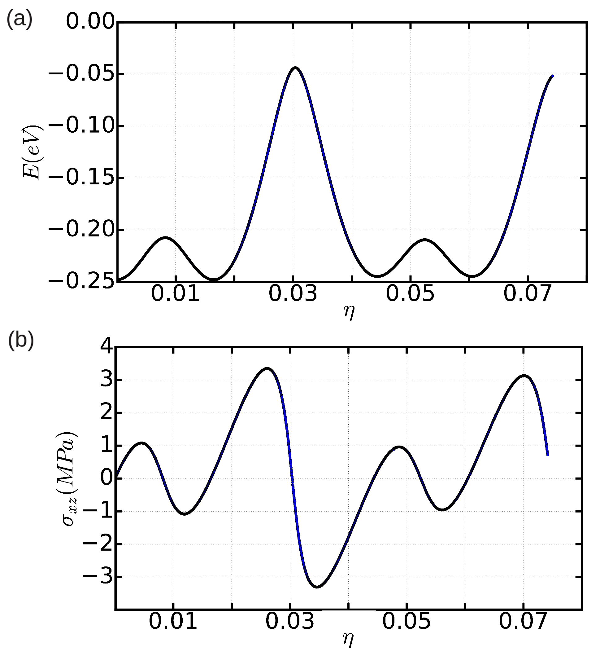
3.2. The Peierls Stress

The Peierls stress, ${\tau }_P$, is key to quantifying the resistance of a crystal to the motion of dislocations. ${\tau }_P$ normally is referred to the critical stress that induces glide of dislocations in the absence of thermal excitations. Here, we use two different methods to evaluate the Peierls stress in our model crystal as concerns the motion of edge dislocations in the basal plane. We note that, since the glide of dislocations involves the breaking and formation of atomic bonds, the value of ${\tau }_P$ in principle is expected to depend strongly on the crystal structure and strength of the interatomic forces.

3.2.1. Method A: Fixed Boundary Conditions

We first employ the usual method found in classical simulation studies based on force fields (see, for instance, Refs. [12,21]), which is briefly described next. The simulation cell is divided into three main parts: “U”, the upper region containing frozen atoms, “L”, the lower region containing frozen atoms, and “M”, the rest of the simulation cell containing mobile atoms (see Figure 6). Regions U and L consist of several layers of atoms that are displaced together as a block. Essentially, a shear strain deformation is applied on the simulation cell perpendicular to the dislocation line and the resulting stresses are monitored. In our particular case, the dislocation line is parallel to the y-axis; hence, we first displace the U slab a small distance along the x-direction, $\Delta u$, and then proceed to minimize the potential energy of the atoms in M while keeping the L slab fixed. Periodic boundary conditions are applied just along the x- and y-directions. The applied mechanical strain is straightforwardly calculated as $\Delta \eta =\Delta u/L_z$, where $L_z$ is the length of the simulation along the z-direction, and the accompanying shear stress is ${\sigma }_{xz}=F_x/L_x{L}_y$, where $F_x$ is the sum of all the forces along the x-direction exerted on the atoms in region U. By iteratively repeating this procedure, we can reproduce with detail the dependence of the shear stress on $\eta$. For small cell distortions, ${\sigma }_{xz}$ is expected to increase almost linearly, as it follows from elastic theory; however, when $\eta$ is large enough so that it induces the glide of dislocations, the shear stress should decrease sharply. The maximum value of ${\sigma }_{xz}$ just before that sudden drop can be identified with the Peierls stress.

In Figure 7, we show the ${\sigma }_{xz}\left(\eta \right)$ results obtained in a large simulation cell containing 344,544 atoms by adopting two different $\Delta \eta$ increments; the thickness of the upper region U, $d_U$, was safely fixed to $5c$ in both cases [21]. As can be appreciated in Figure 7a (case $\Delta \eta$ = 8 × ${10}^{-4}$), a regular pattern emerges that follows elastic theory at small cell deformations (that is, ${\sigma }_{xz}\propto \eta$) and which allows for an estimation of the Peierls stress (as identified with the ${\sigma }_{xz}$ maximum) of ${\tau }_P=6.0\pm 0.1$ MPa. When the employed $\Delta \eta$ is significantly reduced (case $\Delta \eta =1\times {10}^{-4}$, see Figure 7b), the obtained ${\sigma }_{xz}\left(\eta \right)$ curve shows more irregularities and the expected elastic behavior is reproduced at conditions $\eta >0.001$. This outcome reflects the intricacies found in the relaxation of such a large simulation cell, which at small $\eta$ values may easily end up on metastable configurations. In this latter case, we estimate a Peierls stress (as identified with the ${\sigma }_{xz}$ maximum) of ${\tau }_P=7.4\pm 0.1$ MPa.

In order to assess the effects of finite-size bias on the estimation of ${\tau }_P$, we repeated the same calculations in a smaller simulation cell containing n = 18,424 atoms. The stress profiles that we obtained in this case (see Figure 8a) are intricate and do not allow for a clear estimation of the Peierls stress (that is, an unambiguous maximum appearing periodically is missing). Such a finite-size effect is related to the fact that the width of the fcc-like stacking fault is already of the same order of magnitude than the characteristic size of the simulation cell (that is, ∼100 Å). In order to somehow determine ${\tau }_P$ from the results shown in Figure 8a, we monitored the position of the two partial dislocations with the differential displacement (DD) and nearest neighbor (NN) analysis methods (see Section 2.2 and Figure 8b), and averaged the value of the shear stress over the set of strain points at which the partial dislocations change their position. (In the NN case, for the sake of simplicity, we have averaged the position of all the atoms exhibiting a nearest neighbor number different from 12; consequently, we obtain the center position of the stacking fault.) By proceeding like this, we obtained a Peierls stress of ${\tau }_P=1.3\pm 0.2$ MPa, which is about 5 times smaller than the one estimated in the n = 344,544 atoms simulation cell. Our results, therefore, show that finite-size errors affect critically the estimation of ${\tau }_P$ when using Method A (in agreement with previous conclusions by Osetsky and Bacon [21]).

3.2.2. Method B: Periodic Boundary Conditions

As we have just shown in the previous section, Method A requires of very large simulation cells (i.e., $N\sim {10}^5–{10}^6$ atoms) in order to remove all possible finite-size bias affecting the estimation of ${\tau }_P$. This technical aspect suggests that accurate calculation of the Peierls stress with Method A and quantum atomistic or electronic first-principles simulation techniques (in which typically $N\sim {10}^2–{10}^3$ atoms [11,32]) is hardly achievable in practice. Moreover, by construction customary electronic first-principles techniques (e.g., plane-wave density functional theory [5,33]) generally demand the application of periodic boundary conditions in all directions in order to ensure the periodicity and continuity of the electrostatic potential in space. Therefore, it is desirable to work out reliable ${\tau }_P$ computational methods in which all boundaries of the simulation cell are treated equally.

Here, we present a method in which a particular tilt is introduced in the simulation cell containing the edge dislocation and the accompanying change in the total energy is monitored upon constrained relaxation of the system; the relaxation is performed by applying periodic boundary conditions along the three Cartesian directions and optimizing all degrees of freedom of the system except the initial tilt. The resulting stresses then can be calculated numerically with the well-known expressions from elastic theory. (A similar approach has been employed by Wang et al. to investigate the dynamics of screw dislocations in bcc tantalum [34]; in our case, however, the simulations are strictly performed at zero-temperature conditions.) Specifically, the lattice vectors describing our simulation cell are ${\mathbf{a}}_{\mathbf{1}}=(L_x,0,0)$, ${\mathbf{a}}_{\mathbf{2}}=(x_2,L_y,0)$, and ${\mathbf{a}}_{\mathbf{3}}=(x_3,y_3,L_z)$, where $x_3$ represents the introduced tilt. The corresponding shear strain is ${\eta }_{xz}=x_3/L_z$, and the resulting shear stress can be estimated as [35,36,37]:

$${\sigma }_{xz}=\frac{1}{V}\frac{\partial E}{\partial {\eta }_{xz}},$$

(7)

where V represents the volume of the system and E the corresponding total energy.

We enclose the total energy and shear stress results obtained in a simulation cell containing 18,424 atoms in Figure 9a,b. In both cases, the profiles that we obtain as a function of applied shear strain are periodic, in contrast to what we found with Method A when using a simulation cell of the same dimensions (see Figure 8), and elastic behavior is observed for small system deformations. By identifying the global maximum in the ${\sigma }_{xz}$ curve with the Peierls stress, we obtain a value of $3.40\pm 0.01$ MPa (see Figure 9b). This value is roughly two times smaller than the free-of-bias result obtained with Method A in the simulation cell containing n = 344,544 atoms. Therefore, we may conclude that, as compared to Method A, finite-size bias appear to affect less critically the calculation of ${\tau }_P$ with Method B (we recall that, with Method A, we obtained a Peierls stress of $1.3\pm 0.2$ MPa in a same simulation cell containing 18,424 atoms (see previous Section 3.2.1)).

In spite of this favorable outcome, we should acknowledge that the use of periodic boundary conditions in systems containing dislocations is not exempt of important limitations. For instance, periodic boundary conditions are inconsistent with the existence of a net Burgers vector in the simulation cell; consequently, a dipole or quadrupole of dislocations needs to be introduced in the system [38,39]. In order to further incorporate this technical aspect on the calculation of ${\tau }_P$ with Method B, we constructed a large simulation cell of n = 247,680 atoms containing a dislocation quadrupole. Upon introduction of a moderate tilt and by proceeding to relax the system, however, we found that all the dislocations merged into a big stacking fault and were annihilated (we note that a similar behavior has been observed also by Wang et al. in bcc tantalum [34]). This outcome suggests that, unfortunately, even larger simulation cells are required to correct for the inaccuracies associated to Method B.

The main conclusions emerging from Section 3.2.1 and Section 3.2.2 is that the Peierls stress in our model hcp crystal is of the order of 1 MPa. This result is orders of magnitude smaller than the ${\tau }_P$ values reported for archetypal crystals with cubic symmetry (e.g., Fe and Mo) [13]; however, to our surprise, it is very similar in magnitude to the Peierls stresses found in classical metals with the hcp structure (e.g., Zr, Cd, and Mg) [12,13]. Very recently, Landinez-Borda et al. have shown in solid helium that ${\tau }_P$ nominally amounts to zero, that is, dislocations can move freely throughout the crystal in the absence of thermal excitations and shear stresses [11]. The authors of that study have argued that such an effect is quantum in nature as is essentially originated by zero-point fluctuations. Our Peierls stress results obtained in classical rare-gas hcp solids come to corroborate Landinez-Borda et al.’s conclusion, as we have demonstrated that weak interparticle interactions alone cannot render practically vanishing ${\tau }_P$ values.

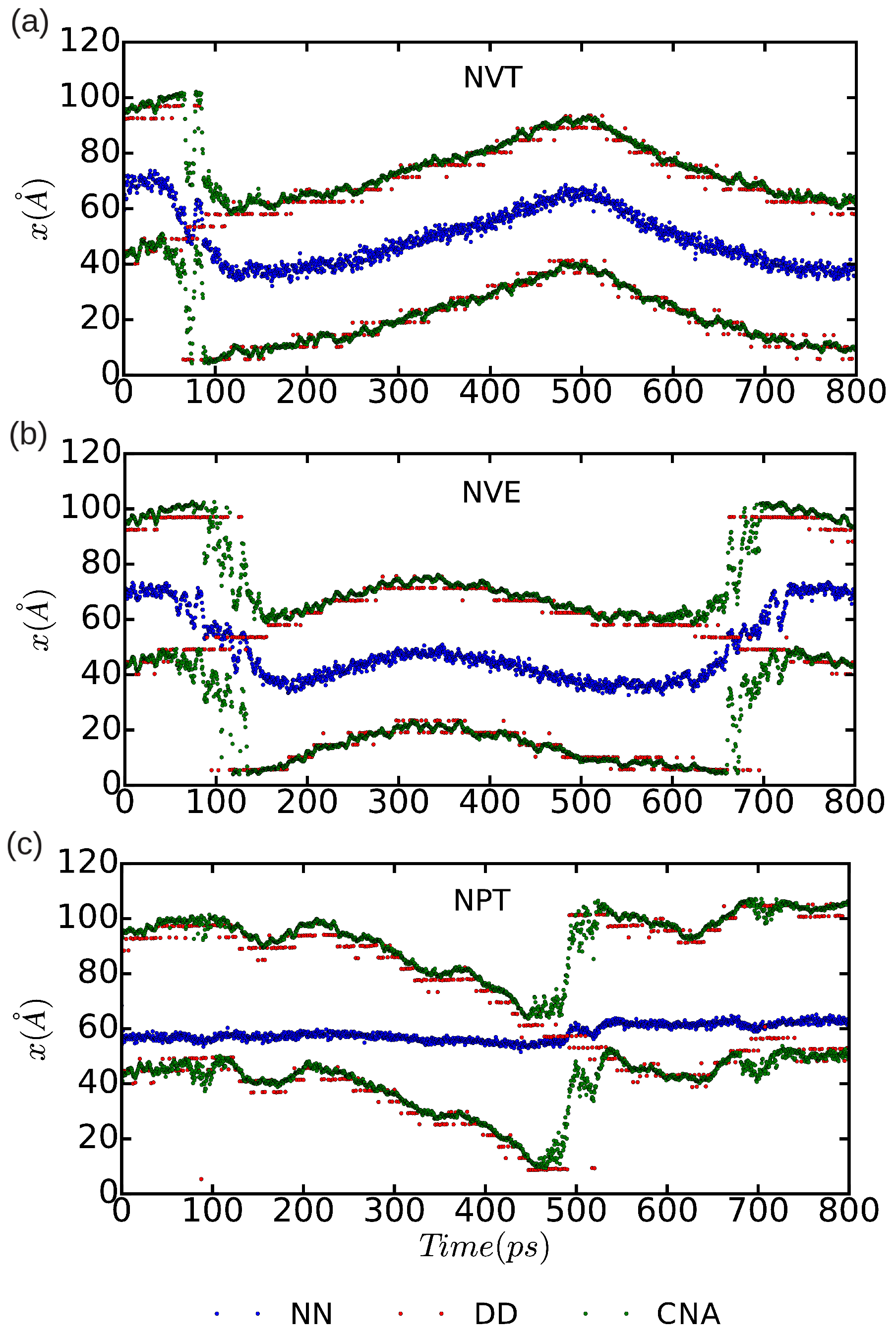
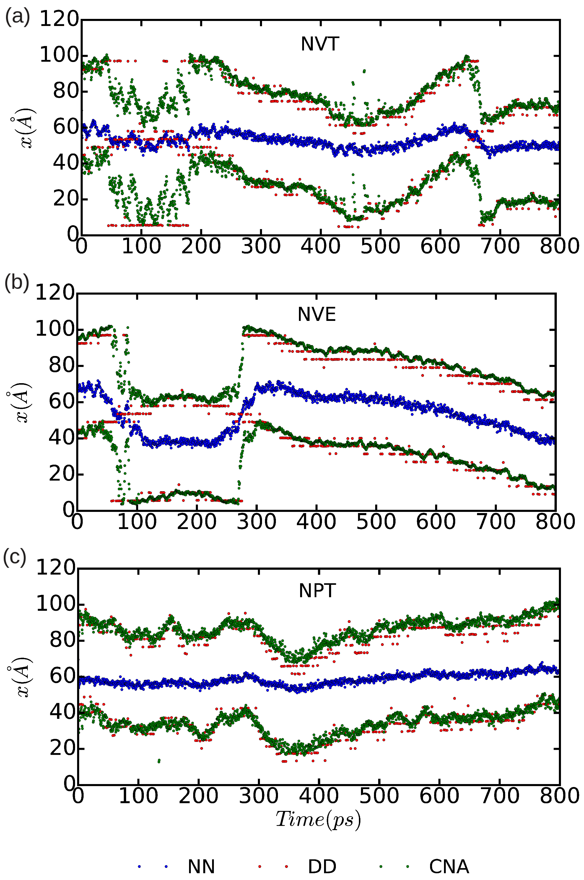
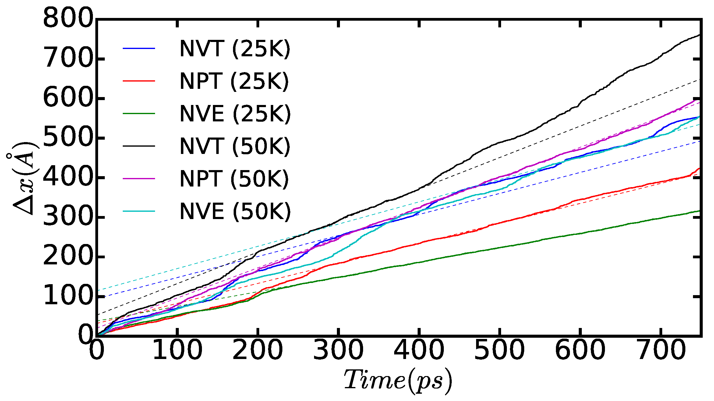
3.3. Dislocation Mobility: Finite-T Simulations

We have estimated the basal mobility of an edge dislocation in our model hcp rare-gas solid at $T\ne 0$ conditions by performing molecular dynamics (MD) simulations in a simulation cell containing n = 18,424 atoms. Fully periodic boundary conditions are employed and a z-vacuum slab is introduced in order to avoid the presence of additional dislocations in the upper and lower edges of the simulation cell (which otherwise would interact with the principal dislocation). No external stresses are considered in our MD simulations, which are performed in the canonical, $(N,V,T)$, microcanonical, $(N,V,E)$, and isothermal-isobaric, $(N,P,T)$ ensembles. For the cases in which the volume is fixed, we use the simulation cell obtained through full geometry relaxation of the system. Likewise, the pressure is set to zero in the $(N,P,T)$ calculations [17]. All simulations are performed with a time step of ${10}^{-3}$ ps and last for a total of 800 ps. The position of the (dissociated) edge dislocation is monitored with three different methods: the differential displacement (DD, Section 2.2.1), the nearest neighbor (NN, Section 2.2.2), and the common neighbor (CNA, Section 2.2.3). In the DD case, due to the high sensitivity of this method to thermal fluctuations, we have averaged the positions of the atoms over five consecutive time steps. In the NN case, for the sake of simplicity, we have averaged the position of the atoms with nearest neighbor number different from 12, hence we have determined the center position of the stacking fault; we note that the NN method provides inaccurate results in the $(N,P,T)$ simulations owing to the fluctuations of the simulation cell, thus that particular case must be disregarded in what follows (shown here just for completitude).

In Figure 10 and Figure 11, we represent the position of the (dissociated) edge dislocation expressed as a function of time at a temperature of 25 and 50 K, respectively. It is appreciated that, in spite of the absence of shear stresses, the dislocation moves at temperatures as low as 25 K, which are well below the corresponding Debye temperature (${\Theta }_D\sim 65$ K [16]). (Cautiously, we have monitored the size of the fluctuating stresses in our MD simulations, which are null in average, and checked that in fact they are not responsible for the observed dislocation glide (e.g., $\mathsf{\sigma }$ fluctuations $\ll {\tau }_P$ in the $(N,P,T)$ runs). The partial dislocations move either to the left or to the right along the x-direction with equal probability, which is fully consistent with the absence of applied stresses. In our MD simulations, the partial dislocations practically remain rigid along the y-direction as no kinks or jogs are observed along their dislocation lines (although for a more detailed analysis of the structural properties of the mobile dislocations the dimensions of our simulation cell should probably need to be increased). It is worth noting that, in the $(N,V,E)$ simulations, we have selected $E=0$ and assigned initial velocities to the atoms reproducing the temperatures chosen in the $(N,V,T)$ and $(N,P,T)$ runs; consequently, after initializing the $(N,V,E)$ simulations, half of the total kinetic energy is transformed into potential and the effective temperature of the system is halved (i.e., $T=12.5$ and 25 K, respectively). In spite of such a reduction in temperature, one still can observe in Figure 9b that the dislocation remains mobile in the $(N,V,E)$ simulations. These results clearly make evident a very low resistance of the rare-gas lattice to dislocation glide. From Figure 10 and Figure 11 we can also estimate the width of the fcc-like stacking fault in our MD simulations, ${\omega }_{sf}$, which corresponds to the position difference between the two dislocation cores. We enclose our averaged ${\omega }_{sf}$ results in

Table 1. Average width of the fcc-like stacking fault, ${\omega }_{sf}$, and edge dislocation diffusion velocity, $v_d$, expressed as a function of temperature, and simulated thermodynamic ensemble (n = 18,424 atoms). ${\omega }_{sf}$ results are expressed in units of lattice parameter a and the figures within parentheses indicate the corresponding statistical uncertainty.

T = 25 K
	$v_d(\mathrm{m}/\mathrm{s})$	${\omega }_{sf}\left(a\right)$
$\mathrm{NVT}$	$57.2\left(0.5\right)$	$12.0\left(0.3\right)$
$\mathrm{NVE}$	$37.0\left(0.5\right)$	$12.1\left(0.6\right)$
$\mathrm{NPT}$	$53.1\left(0.5\right)$	$12.1\left(0.6\right)$
T = 50 K
	$v_d(\mathrm{m}/\mathrm{s})$	${\omega }_{sf}\left(a\right)$
$\mathrm{NVT}$	$79.6\left(0.5\right)$	$11.9\left(3.3\right)$
$\mathrm{NVE}$	$56.2\left(0.5\right)$	$11.9\left(3.3\right)$
$\mathrm{NPT}$	$76.1\left(0.5\right)$	$11.9\left(3.3\right)$

, expressed as a function of temperature and simulation ensemble. It is appreciated that all three ensembles provide consistent results and that, as expected, thermal excitations tend to increase the ${\omega }_{sf}$ fluctuations.

In Figure 12, we show the time-accumulated average displacement of the dissociated edge dislocations, $\Delta x$, expressed as a function of time, temperature, and simulation ensemble. In particular, we calculate this quantity with the formula:

$$\Delta x\left(t\right)=\left|x\right(t)-x(t-\delta t\left)\right|+\Delta x(t-\delta t),$$

(8)

where $x\left(t\right)$ corresponds to the average position of the atoms belonging to the dislocations along the x direction at time t (that is, as shown in Figure 10 and Figure 11) and $\delta t$ is equal to a time step in our molecular dynamic simulations. A series of kinks appear in the figure that are a consequence of the dislocation cores passing through the boundaries of the simulation cell (that is, due to use of periodic boundary conditions during the crossing of an edge, some of the atoms belonging to the same dislocation core are located in one extreme of the box, whereas the rest remain in the opposite boundary). From the slope of the linear fits to the $\Delta x$ data points, which are not affected by such a periodic boundary artifact, we can deduce the module of the average diffusion velocity of the dislocations, $v_d$, as a function of temperature and simulated thermodynamic ensemble. The results enclosed in Table 1 show that simulations performed both in the $(N,V,T)$ and $(N,P,T)$ ensembles render very similar $v_d$ values; by contrast, simulations performed in the $(N,V,E)$ ensemble systematically provide smaller dislocation diffusion velocities due to the effective reduction in the temperature of the system (see preceding paragraph). Interestingly, our MD results suggest a square root-like dependence of $v_d$ on temperature, $v_d\propto \sqrt{T}$. For instance, in the $(N,V,T)$ and $(N,P,T)$ cases, we realize that $v_d\left(2T\right)\simeq \sqrt{2}{v}_d\left(T\right)$, and, when comparing those results with the values obtained in the $(N,V,E)$ ensemble, we consistently find that $v_d^{NVT}\left(T\right)\simeq \sqrt{2}{v}_d^{NVE}\left(T\right)$. This behavior appears to depart significantly from the Arrhenius-like relation that is expected for thermally activated dislocations, namely $v_d\propto \exp [-\Delta G/k_{B}T]$, and which has been observed in other materials at high temperatures [2,40,41].

It is physically insightful to compare the $v_d$ values obtained in our model rare-gas solid with those reported for other materials with the hcp structure. In the case of Zr, Khater and Bacon have estimated edge dislocation velocities within the basal plane of about 100 ms${}^{-1}$ at room temperature and practically vanishing applied shear stresses (see Figure 7a in Ref. [12]). In the present case, similar $v_d$ values are obtained already at a much lower temperature of 50 K and nominally zero mechanical stress. This comparison comes to show that edge dislocations in classical hcp rare-gas solids are much more mobile than in structurally analogous metals. The origins of such differences may reside on the interatomic interactions (mind that the atomic masses of Zr and Xe atoms are roughly comparable), which in the case of rare gases are extremely weak [33].

4. Conclusions

We have presented a comprehensive computational study on the structural and mobility properties of edge dislocations in classical rare-gas solid with the hcp structure. We have shown that dissociation of edge dislocations into Shockley partials, as induced by the presence of a low-energy metastable stacking fault, is a common process in hcp rare-gas crystals. On the other hand, we have inferred that quantum nuclear effects further enhance the dissociation of edge dislocations into partials as they tend to decrease the energy of the actual stacking fault. A dislocation-related quantity that indirectly appears to be drastically affected by quantum nuclear effects is the Peierls stress, ${\tau }_P$. While we have calculated a Peierls stress value of the order of 1 MPa in our model classical rare-gas crystal, other researchers have estimated a practically vanishing ${\tau }_P$ in archetypal quantum crystal hcp ${}^4$He. Meanwhile, the mobility of edge dislocations in rare-gas solids in general is very large, owing to the characteristic weak interactions between atoms. In the present case, we have found that glide of dislocations can be activated at temperatures as low as ∼10 K in the absence of any applied shear stress, achieving large dislocation diffusion velocities of the order of 10 ms${}^{-1}$. Furthermore, our molecular dynamics results suggest that the diffusion velocity of edge dislocations depends on temperature as the square root, namely $v_d\propto \sqrt{T}$, in contrast to what has been observed in other crystals. The conclusions presented in this study provide valuable new insights into the structure and mobility of edge dislocations in rare-gas solids, and allow for a quantitative assessment of the importance of quantum nuclear effects in solid ${}^4$He dislocation behavior.

References

1. Hirth, J.P.; Lothe, J. Theory of Dislocations, 2nd ed.; John Wiley: New York, NY, USA, 1982. [Google Scholar]
2. Hull, D.; Bacon, D.J. Introduction to Dislocations, 5th ed.; Elsevier: Amsterdam, The Netherlands, 2011. [Google Scholar]
3. Bulatov, V.V.; Cai, W. Computer Simulations of Dislocations; Oxford University Press: Oxford, UK, 2006. [Google Scholar]
4. Nabarro, F.; Kubin, L.; Hirth, J. Dislocations in Solids; Elsevier: Amsterdam, The Netherlands, 2009; Volumes 1–13, pp. 14–16. [Google Scholar]
5. Cazorla, C.; Boronat, J. Simulation and understanding of atomic and molecular quantum crystals. Rev. Mod. Phys. 2017, 89, 035003. [Google Scholar] [CrossRef]
6. Ceperley, D.M. Path integrals in the theory of condensed helium. Rev. Mod. Phys. 1995, 67, 279. [Google Scholar] [CrossRef]
7. McMahon, J.M.; Morales, M.A.; Pierleoni, C.; Ceperley, D.M. The properties of hydrogen and helium under extreme conditions. Rev. Mod. Phys. 2012, 84, 1607. [Google Scholar] [CrossRef]
8. Herrero, C.P.; Ramírez, R. Path-integral simulation of solids. J. Phys. Condens. Matter 2014, 26, 233201. [Google Scholar] [CrossRef] [PubMed]
9. Cazorla, C.; Boronat, J. First-principles modeling of quantum nuclear effects and atomic interactions in solid 4He at high pressure. Phys. Rev. B 2015, 91, 024103. [Google Scholar] [CrossRef]
10. Haziot, A.; Rojas, X.; Fefferman, A.D.; Beamish, J.R.; Balibar, S. Giant plasticity of a quantum crystal. Phys. Rev. Lett. 2013, 110, 035301. [Google Scholar] [CrossRef] [PubMed]
11. Landinez-Borda, E.J.; Cai, W.; de Koning, M. Dislocation Structure and Mobility in hcp 4He. Phys. Rev. Lett. 2016, 117, 045301. [Google Scholar] [CrossRef] [PubMed]
12. Khater, H.A.; Bacon, D.J. Dislocation core structure and dynamics in two atomic models of α-zirconium. Acta Mater. 2010, 58, 2978–2987. [Google Scholar] [CrossRef]
13. Kamimura, Y.; Edagawa, J.; Takeuchi, S. Experimental evaluation of the Peierls stresses in a variety of crystals and their relation to the crystal structure. Acta Mater. 2013, 61, 294–309. [Google Scholar] [CrossRef]
14. Fefferman, A.D.; Souris, F.; Haziot, A.; Beamish, J.R.; Balibar, S. Dislocation networks in 4He crystals. Phys. Rev. B 2014, 89, 014105. [Google Scholar] [CrossRef]
15. Balibar, S.; Beamish, J.; Fefferman, A.D.; Haziot, A.; Rojas, X.; Souris, F.C.R. Dislocations in a quantum crystal: Solid helium: A model and an exception. Physique 2016, 17, 264–275. [Google Scholar] [CrossRef] [Green Version]
16. Fenichel, H.; Serin, B. Low-temperature specific heats of solid neon and solid xenon. Phys. Rev. 1966, 142, 490. [Google Scholar] [CrossRef]
17. Plimpton, S. LAMMPS Molecular Dynamics Simulator. J. Comput. Phys. 1995, 117, 1. Available online: http://lammps.sandia.gov (accessed on 13 December 2017). [CrossRef]
18. Packard, J.R.; Swenson, C.A. An experimental equation of state for solid xenon. J. Phys. Chem. Solids 1963, 24, 1405–1418. [Google Scholar] [CrossRef]
19. Pollack, G.L. The solid state of rare gases. Rev. Mod. Phys. 1964, 36, 748. [Google Scholar] [CrossRef]
20. Bernades, N. Quantum Mechanical Law of Corresponding States for Van der Waals Solids at 0° K. Phys. Rev. 1960, 120, 807. [Google Scholar] [CrossRef]
21. Osetsky, Y.N.; Bacon, D.J. An atomic-level model for studying the dynamics of edge dislocations in metals. Model. Simul. Mater. Sci. Eng. 2003, 11, 427. [Google Scholar] [CrossRef]
22. Vitek, V. Structure of dislocation cores in metallic materials and its impact on their plastic behaviour. Prog. Mater. Sci. 1992, 36, 1–27. [Google Scholar] [CrossRef]
23. Stukowski, A. Structure identification methods for atomistic simulations of crystalline materials. Model. Simul. Mater. Sci. Eng. 2012, 20, 045021. [Google Scholar] [CrossRef]
24. Honeycutt, J.D.; Andersen, H.C. Molecular dynamics study of melting and freezing of small Lennard-Jones clusters. J. Phys. Chem. 1987, 91, 4950–4963. [Google Scholar] [CrossRef]
25. Bacon, D.J.; Vitek, V. Atomic-scale modeling of dislocations and related properties in the hexagonal-close-packed metals. Metall. Mater. Trans. A 2002, 33, 721–733. [Google Scholar] [CrossRef]
26. Boninsegni, M.; Kuklov, A.B.; Pollet, L.; Prokofev, N.V.; Svistunov, B.V.; Troyer, M. Luttinger liquid in the core of a screw dislocation in helium-4. Phys. Rev. Lett. 2007, 99, 035301. [Google Scholar] [CrossRef] [PubMed]
27. Ackland, G.J.; Wooding, S.J.; Bacon, D.J. Defect, surface and displacement-threshold properties of α-zirconium simulated with a many-body potential. Philos. Mag. A 1995, 71, 553–565. [Google Scholar] [CrossRef]
28. Mendelev, M.I.; Ackland, G.J. Development of an interatomic potential for the simulation of phase transformations in zirconium. Philos. Mag. Lett. 2007, 87, 349–359. [Google Scholar] [CrossRef]
29. Keyse, R.J.; Venables, J.A. Stacking fault energy and crystal stability of solid krypton and xenon. J. Phys. C Sol. Stat. Phys. 1985, 18, 4435. [Google Scholar] [CrossRef]
30. Cazorla, C.; Boronat, J. Atomic kinetic energy, momentum distribution, and structure of solid neon at zero temperature. Phys. Rev. B 2008, 77, 024310. [Google Scholar] [CrossRef]
31. Boronat, J.; Cazorla, C.; Colognesi, D.; Zoppi, M. Quantum hydrogen vibrational dynamics in LiH: Neutron-scattering measurements and variational Monte Carlo simulations. Phys. Rev. B 2004, 69, 174302. [Google Scholar] [CrossRef]
32. Shin, I.; Carter, E.A. Possible origin of the discrepancy in Peierls stresses of fcc metals: First-principles simulations of dislocation mobility in aluminum. Phys. Rev. B 2013, 88, 064106. [Google Scholar] [CrossRef]
33. Cazorla, C. The role of density functional theory methods in the prediction of nanostructured gas-adsorbent materials. Coord. Chem. Rev. 2015, 300, 142–163. [Google Scholar] [CrossRef]
34. Wang, G.; Strachan, A.; Cagin, T.; Goodard, W.A., III. Calculating the Peierls energy and Peierls stress from atomistic simulations of screw dislocation dynamics: application to bcc tantalum. Model. Simul. Mater. Sci. Eng. 2004, 12, S371. [Google Scholar] [CrossRef]
35. Born, M.; Huang, K. Dynamical Theory of Crystal Lattices; Oxford University Press: New York, NY, USA, 1954. [Google Scholar]
36. Cazorla, C.; Lutsyshyn, Y.; Boronat, J. Elastic constants of solid 4He under pressure: Diffusion Monte Carlo study. Phys. Rev. B 2012, 85, 024101. [Google Scholar] [CrossRef]
37. Cazorla, C.; Lutsyshyn, Y.; Boronat, J. Elastic constants of incommensurate solid 4He from diffusion Monte Carlo simulations. Phys. Rev. B 2013, 87, 214522. [Google Scholar] [CrossRef]
38. Olmsted, D.; Hardikar, K.Y.; Phillips, R. Lattice resistance and Peierls stress in finite size atomistic dislocation simulations. Model. Simul. Mater. Sci. Eng. 2001, 9, 215. [Google Scholar] [CrossRef]
39. Yadav, S.K.; Ramprasad, R.; Misra, A.; Liu, X.-Y. Core structure and Peierls stress of edge and screw dislocations in TiN: A density functional theory study. Acta Mater. 2014, 74, 268–277. [Google Scholar] [CrossRef]
40. Balasubramanian, N. The temperature dependence of the dislocation velocity-stress exponent. Scr. Metall. 1996, 3, 21–24. [Google Scholar] [CrossRef]
41. Fitzgerald, S.P. Kink pair production and dislocation motion. Sci. Rep. 2016, 6, 39708. [Google Scholar] [CrossRef] [PubMed]
Figure 1. Sketch of a fully relaxed system containing an edge dislocation from different views. Green spheres represent atoms belonging to the dislocation core, blue spheres atoms belonging to the fcc-like stacking fault, and yellow spheres atoms with common hcp atomic coordination features. Red arrows represent the Burgers vectors of the partial dislocations. (a,b) represent different views of the simulation cell.
Crystals 08 00064 g001
Figure 2. Relative displacement (a,b) and differential displacement (c,d) of the atoms above and below the glide plane of the edge dislocation in the x- and y-directions. The simulation cell contains n = 344,544 atoms and is fully relaxed.
Crystals 08 00064 g002
Figure 3. Relative displacement (a,b) and differential displacement (c,d) of the atoms above and below the glide plane of the edge dislocation in the x and y directions. The simulation cell contains n = 18,424 atoms. Green and blue lines represent the results obtained in a non-relaxed ( σ i j 0 ) and a fully relaxed ( σ i j = 0 ) simulation cell, respectively.
Crystals 08 00064 g003
Figure 4. Relative displacement (a,b) and differential displacement (c,d) of the atoms above and below the glide plane of the edge dislocation in the x- and y-directions. The simulation cell contains n = 1368 atoms and is fully relaxed.
Crystals 08 00064 g004
Figure 5. The γ -surface of the analyzed classical hcp rare-gas crystal. Perfect hcp stacking positions correspond to the four corners of the plot while large white spheres indicate metastable fault positions. Iso- γ curves are represented with solid black lines at 5 and 10 mJ/m 2 intervals.
Crystals 08 00064 g005
Figure 6. Sketch of the system used to estimate the Peierls stress with Method A. Three main parts are differentiated: the upper part “U”, the lower part “L”, and the region with mobile atoms “M”. “P” indicates application of periodic boundary conditions and the dashed line the orientation of the edge dislocation.
Crystals 08 00064 g006
Figure 7. Evolution of the shear stress expressed as a function of strain for a simulation cell containing n = 344,544 atoms in which the thickness of the “U” region is taken to be d U = 5 c . Results obtained with Δ η = 8 × 10 4 and 1 × 10 4 are shown in (a,b), respectively (see text).
Crystals 08 00064 g007
Figure 8. (a) evolution of the shear stress expressed as a function of strain for a simulation cell containing n = 18,424 atoms in which the thickness of the “U” part is equal to d U = 2.5 c . Several mechanical strain steps, Δ ϵ , are considered; (b) position of the corresponding dissociated edge dislocation expressed as a function of strain. “DD” and “NN” stand for the analysis methods of differential displacement and nearest neighbors, respectively.
Crystals 08 00064 g008
Figure 9. Energy (a) and shear stress (b) expressed as a function of shear strain for a simulation cell containing n = 18,424 atoms in which periodic boundary conditions are applied along the three Cartesian directions.
Crystals 08 00064 g009
Figure 10. Position of the dissociated edge dislocation expressed as a function of time for a simulation cell containing n = 18,424 atoms. Molecular dynamics simulations have been performed in the three thermodynamic ensembles (a) N V T , (b) N V E , and (c) N P T ; the temperature has been fixed to 25 K, the pressure to zero, and the volume to the equilibrium one. In the N V E case, an equilibrium temperature of 12.5 K is reached. “DD”, “NN”, and “CNA” stand for the analysis methods of differential displacement, nearest neighbors, and common neighbor, respectively.
Crystals 08 00064 g010
Figure 11. Position of the edge dissociated dislocation expressed as a function of time for a simulation cell containing N = 18424 atoms. Molecular dynamics simulations have been performed in the three thermodynamic ensembles (a) N V T , (b) N V E , and (c) N P T ; the temperature has been fixed to 50 K, the pressure to zero, and the volume to the equilibrium one. In the N V E case, an equilibrium temperature of 25 K is reached. “DD”, “NN”, and “CNA” stand for the analysis methods of differential displacement, nearest neighbors, and common neighbor, respectively.
Crystals 08 00064 g011
Figure 12. Time-accumulated average displacement of the dissociated edge dislocations expressed as a function of time, temperature, and simulated thermodynamic ensemble (n = 18,424 atoms). Solid lines represent the actual dislocation positions and dashed lines are linear fits performed on regions in which the dislocation motion is not disturbed by the simulation cell boundaries. Dislocation diffusion velocities are deduced directly from the slope of the linear fits.
Crystals 08 00064 g012