Article

An Approach for Defect Detection in Friction Stir Welding Based on the Welding Force and Machine Learning

1
School of Computer Software, Tianjin University, Tianjin 300072, China
2
School of Materials Science and Engineering, Tianjin University, Tianjin 300072, China
*
Author to whom correspondence should be addressed.
Crystals 2026, 16(9), 573; https://doi.org/10.3390/cryst16090573
Submission received: 22 July 2026 / Revised: 28 August 2026 / Accepted: 31 August 2026 / Published: 2 September 2026
(This article belongs to the Section Crystalline Metals and Alloys)

Abstract

This study leverages multiple machine learning algorithms for defect detection in friction stir welding (FSW), utilizing force-derived features as model inputs. Furthermore, the underlying relationships between welding forces and defect formation were systematically investigated, alongside an evaluation of the efficacy of force-feature-driven defect detection models. Results indicated that the variations in the averages and waveforms in the traverse force ( F x ), lateral force ( F y ) and plunge force ( F z ) are highly responsible for the defect formation in FSW joints, such that an increase in F y causes waveform distortions in F x and F y . F y a v g is the most important feature for the defect formation for 724 sets of experimental data. Defect detection based on thresholding of Fyavg and Fzavg achieves an accuracy of 80.3%. In contrast, four machine learning algorithms—Decision Tree (DT), K-Nearest Neighbors (KNNs), Support Vector Machine (SVM), and Artificial Neural Network (ANN)—were employed to construct defect detection models using the extracted force features as inputs, yielding accuracies of 93.5%, 97.5%, 95.7% and 94.9%, respectively. These findings further elucidate the underlying mechanics, that is, Fx and Fy primarily originated from the extrusion and shear forces induced by the probe’s rotation and traverse, whereas Fz was predominantly attributed to the compressive action of the shoulder.

1. Introduction

Friction stir welding (FSW), as a solid-state joining technique, has been extensively adopted for fabricating aluminum alloy structures in the rail transportation, aerospace, and automotive industries [1,2,3,4]. Driven by its increasing deployment in mass production and large-scale structural fabrication in recent years, there is a growing demand for intelligent FSW systems to enhance weld quality while reducing production costs. Accurate defect detection serves as a cornerstone of such intelligent FSW implementations. However, defect formation during welding is governed by a multitude of factors, including suboptimal welding parameters, tool wear, assembly gaps, and workpiece dimensional deviations [5,6,7]. No universally applicable methodology currently exists for defect detection under complex welding conditions.
Prior studies indicate that critical signatures of defect formation are intrinsically encoded within key process variables, such as welding force, temperature, and torque. Consequently, deciphering the relationships between these variables and defect generation represents a promising avenue for the development of robust defect detection strategies. Among these, the welding force comprising traverse force (Fx), lateral force (Fy), and plunge force (Fz) has received increasing attention within the materials joining community due to its direct correlation with tool–workpiece interaction mechanics [8,9,10]. Several force features have been reported to exhibit strong correlations with welding defects [11,12,13,14,15]. Das et al. [11] reported that the power spectral density of Fx and Fz for the FSW joints with tunnel defects was higher than those for defect-free FSW joints. Guan et al. [12] proposed that the reduction in the wave crests of Fx corresponded well with tunnel defects. Frank et al. [13] demonstrated that the ratio of the third-harmonic amplitude to the first-harmonic amplitude in the Fx signal can be used to identify defects, with the defect size exhibiting a linear correlation with this ratio relative to the mean value of Fx. Additionally, the variance and mean squared error of the detail coefficients derived from Fz enabled effective localization of surface defects [14,15]. However, the validity of these conclusions was established on the basis of relatively small datasets, with a maximum of only 28 training samples considered. Consequently, the generalizability of these features for defect detection cannot be guaranteed across joints fabricated over a broader range of welding parameters.
Machine learning leverages classification and regression algorithms to extract latent patterns from empirical data, thereby addressing nonlinear and complex problems. Regarding FSW, machine learning approaches have been employed for defect detection and joint property prediction [16,17,18,19,20,21,22]. Specifically, welding parameters containing rotation speed, traverse speed, and plunge depth have been utilized to drive the regression models for predicting the tensile properties of welded joints [16,17,18]. Sudhagar et al. [19] used the features from a surface image as the input of machine learning to build a defect detection model. Dhanraj et al. [20] employed the statistical characteristics from the vibration patterns to predict the surface defects with several classification algorithms. Du et al. [21,22] used the four causative variables from numerical simulation results, including temperature, strain rate, torque, and shear stress, to identify tool failure and void defects. Among the investigated variables, the maximum shear stress exerted the most dominant influence on void formation. These findings underscore the potential of machine learning in constructing robust defect detection models, provided that sufficiently large and representative training datasets are available. Furthermore, to facilitate real-time implementation, the input variables employed in these models should be both directly measurable and readily accessible during the welding process.
In this study, a force-feature-driven machine learning approach is investigated for defect detection in FSW. A customized three-axis force-sensing system was developed to acquire in situ Fx, Fy, and Fz signals throughout the welding process, with a particular emphasis on characterizing internal defects such as voids and tunnel defects. The correlations between welding force signatures and defect formation were systematically analyzed by metallographic examination of joint cross-sections in conjunction with a comparative assessment of the corresponding force signal variations. Subsequently, a hybrid set of time- and frequency-domain force features was extracted to serve as inputs for four machine learning algorithms, enabling effective classification of defect-free and defective joints.

2. Experiment

2.1. FSW Experiment

The base material employed in this study was 5A06 aluminum alloy, with dimensions of 150 mm × 250 mm × 8 mm. A total of 185 welding experiments were conducted across a wide range of process parameters, specifically rotation speeds of 350–1400 rpm and traverse speeds of 80–720 mm/min. The FSW tool featured a concave shoulder with a diameter of 18 mm and a threaded pin of 7.9 mm in length, incorporating three flats. Throughout the welding process, the three-axis force transducers acquired in situ Fx, Fy, and Fz signals at a sampling frequency of 7800 Hz. The performance specifications of the force measurement system are summarized in Table 1. The proportions of the three-dimensional forces driven by the shoulder and the pin are calculated based on the variations in the 3D force data before and after pin fracture. Prior to fracture, the measured 3D forces represent the combined contribution of both the shoulder and the pin acting on the weld material. Following fracture, the measured forces were solely attributed to the shoulder acting on the surface material of the weld. Consequently, the reduction in the 3D forces across the fracture event corresponded to the forces exerted specifically by the pin on the weld material. Six metallographic specimens were extracted from each welded plate at uniform 30 mm intervals. The cross-sections were subsequently examined using an optical microscope to characterize internal defect morphology. A comparative analysis was then conducted on the welding force signatures and their dynamic variations between defect-free and defective joints. From these force signals, fifteen time-domain features and nine frequency-domain features were systematically extracted via mathematical formulations and fast Fourier transform (FFT), respectively. Twenty-four force features were extracted from the in situ Fx, Fy, and Fz signals. For each force component, five time-domain features were computed: mean, range, standard deviation, skewness, and kurtosis. Three frequency-domain features—the first, second, and third harmonic amplitudes—were derived via fast Fourier transform (FFT). While the time-domain features characterize the statistical distribution of the force signals, the frequency-domain features elucidate the periodic modulation inherent in the tool–workpiece interaction. Detailed definitions and schematic illustrations are presented in Table 2. Feature extraction was conducted on the steady-state segment of each welding case using a one-second sliding window. Subsequently, all features were normalized to the range [0, 1] to facilitate model training. The definitions of these features are listed in Table 2.
It is worth noting that the samples were mechanically polished and etched with Keller’s reagent (2 mL HF + 5 mL HNO3 + 3 mL HCl + 90 mL distilled water) for 15 s. The cross-sections were characterized using the VHX-2000C microscope (KEYENCE, OSAKA, Japan). Defect size was quantified from the cross-sectional images by grayscale conversion and thresholding in MATLAB 2023B. The fixed threshold (grayscale value < 0.3) was applied to segment defect zones. Then, the projected defect area was calculated by counting pixels below the threshold and converted to the actual area through pixel calibration. Defect labels were assigned automatically according to the program: specimens with a projected defect area of 0 mm2 were labeled defect-free, and those with an area >0 mm2 were labeled defective.

2.2. Machine Learning

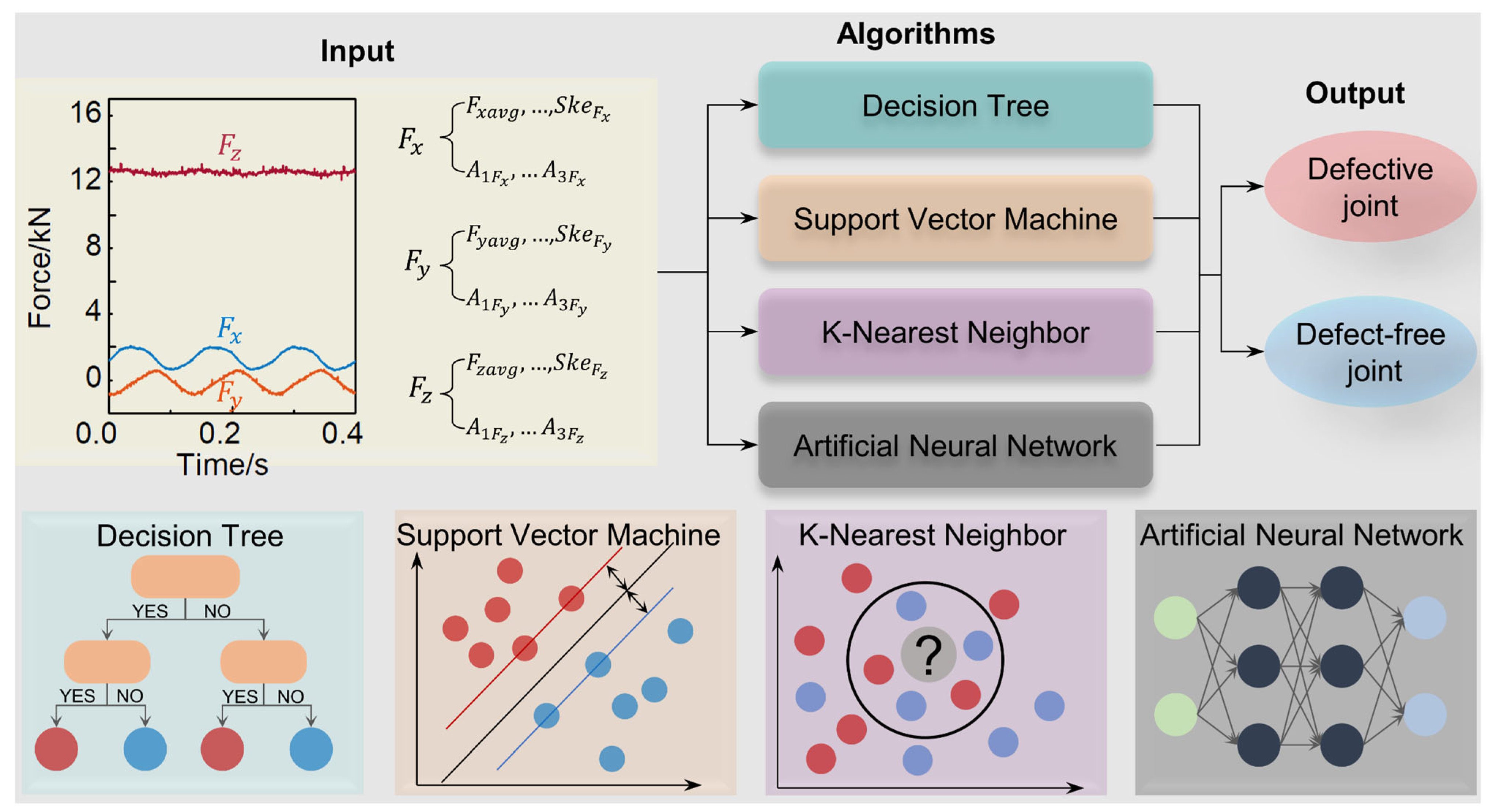
A dataset comprising 681 defect-free and 362 defective samples was curated from the 185 welding experiments. To mitigate class imbalance and eliminate sampling bias, 362 defect-free samples were randomly chosen to match the defective cohort. Subsequently, four machine learning algorithms, namely Decision Tree (DT), Support Vector Machine (SVM), K-Nearest Neighbors (KNNs), and Artificial Neural Network (ANN), were employed to classify the joint integrity. The workflow of the machine learning framework is illustrated in Figure 1, which utilizes normalized force features as inputs and defect classification labels as outputs. The welding force in the FSW processing is schematically diagramed in Figure 2. For model training and validation, 580 and 144 samples were randomly allocated to the training and testing sets, respectively. The four classification algorithms (summarized in Table 3) are described as follows:
  • In the DT model, each non-leaf node is responsible for a specific feature, while each leaf node stores a probability distribution corresponding to the predicted class labels. This hierarchical tree structure renders the underlying decision-making process intrinsically interpretable, as classification proceeds via a transparent sequence of feature-based splits from the root node to the terminal leaves.
  • SVM constructs an optimal separating hyperplane by identifying critical training samples known as support vectors. The objective is to maximize the margin, defined as the aggregate of the minimum distances from the training data to the hyperplane, thereby enhancing the model’s generalization capability.
  • KNN operates on the principle of locality, classifying unlabeled samples by minimizing the distance to their k-nearest training observations. The class label of a test sample is determined through a majority voting scheme based on the labels of its closest neighbors in the feature space.
  • ANN emulates the information-processing mechanisms of biological neural systems and typically comprises three fundamental layers: an input layer, one or more hidden layers, and an output layer. Within the hidden layers, computational nodes receive input signals and iteratively optimize the network parameters—including the weight matrix, activation function, and bias vector—to minimize prediction error during training.
Results of the machine learning models were presented with a confusion matrix, including true positive (TP), false positive (FP), true negative (TN) and false negative (FN). TP and TN are the correct predictions, and FP and FN are the incorrect predictions. Three statistic metrics, containing accuracy, precision and recall, were calculated according to the following equations:
A c c u r a c y = T P + T N T N + F N + T P + F P
P r e c i s i o n = T P T P + F P
R e c a l l = T P T P + F N

3. Results

3.1. Force Signals

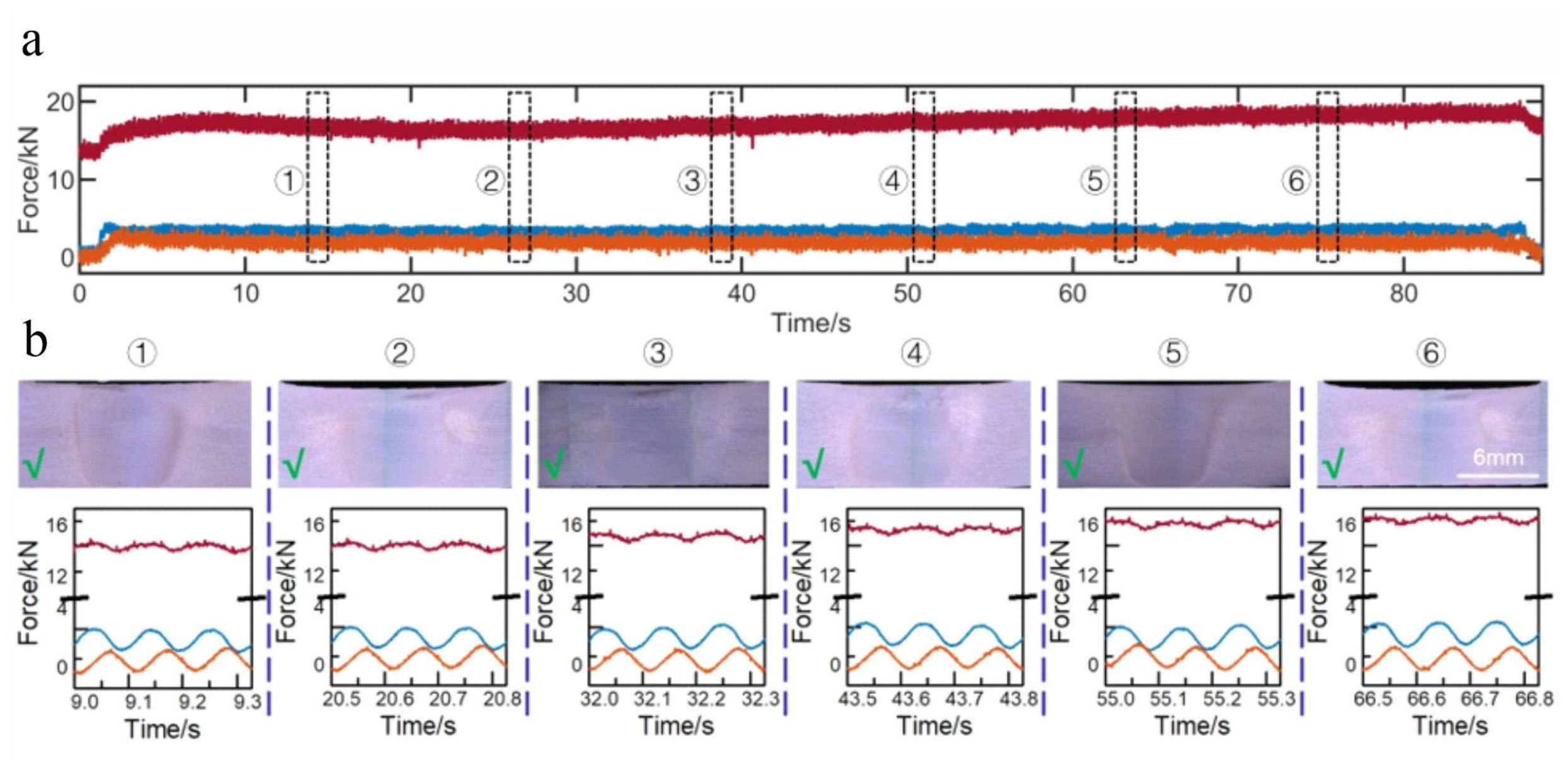
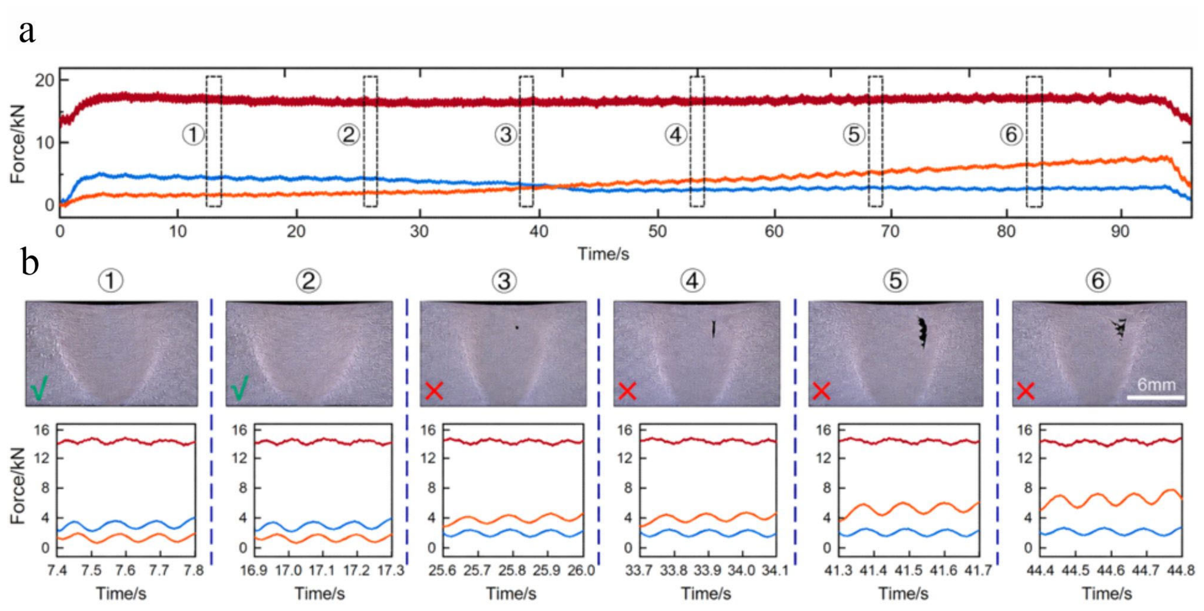
Figure 3 presents the welding force curves and corresponding cross-sectional macrographs of joints fabricated at 550 rpm and 160 mm/min. As evidenced in Figure 3a, Fz exhibits a marginal decrement during the initial 15 s, corresponding to the transient phase prior to the establishment of a fully stabilized welding state. Throughout the subsequent steady-state welding stage, Fx, Fy, and Fz maintain mean values of 14.2 kN, 1.8 kN, and 0.5 kN, respectively. Figure 3b illustrates the magnified force signals for six defect-free joints, correlated with their cross-sectional profiles. Both Fx and Fy display periodic fluctuations at a frequency of 9 Hz, equivalent to the tool rotation frequency, exhibiting a distinct phase difference of 1/4 period. Their waveforms are approximately sinusoidal, whereas Fz remains relatively stable with negligible oscillation. While no discernible variations in Fx and Fy are observed across the six joints at different longitudinal locations, Fz demonstrates a progressive decrement from 14.3 kN to 12.6 kN.
Figure 4a illustrates the force responses for the joint welded at 550 rpm and 240 mm/min. While Fx and Fz remain relatively stable at approximately 3.0 kN and 14.2 kN, respectively, Fy exhibits an anomalous increase from 3.4 kN to 4.1 kN at approximately 20 s. This transient deviation is likely attributable to variations in assembly accuracy or workpiece dimensional tolerances. As evidenced in Figure 4b, the FSW joint remains defect-free prior to this fluctuation in Fy. However, once Fy rises to 3.5 kN, slightly surpassing Fx, a void defect emerged on the advancing side (AS) of the joint. A comparative analysis of four defective joints reveals that the differential force (ΔF = FxFy) measures 1.4 kN, 1.8 kN, 2.5 kN, and 3.2 kN, respectively, all of which are substantially lower than those observed in the two defect-free counterparts. This trend indicates a strong correlation between the reduction in ΔF and defect formation. Furthermore, relative to the force profiles in Figure 3a, the combined effect of a diminished ΔF and elevated force amplitudes suggests a heightened susceptibility to defect formation under these welding conditions.
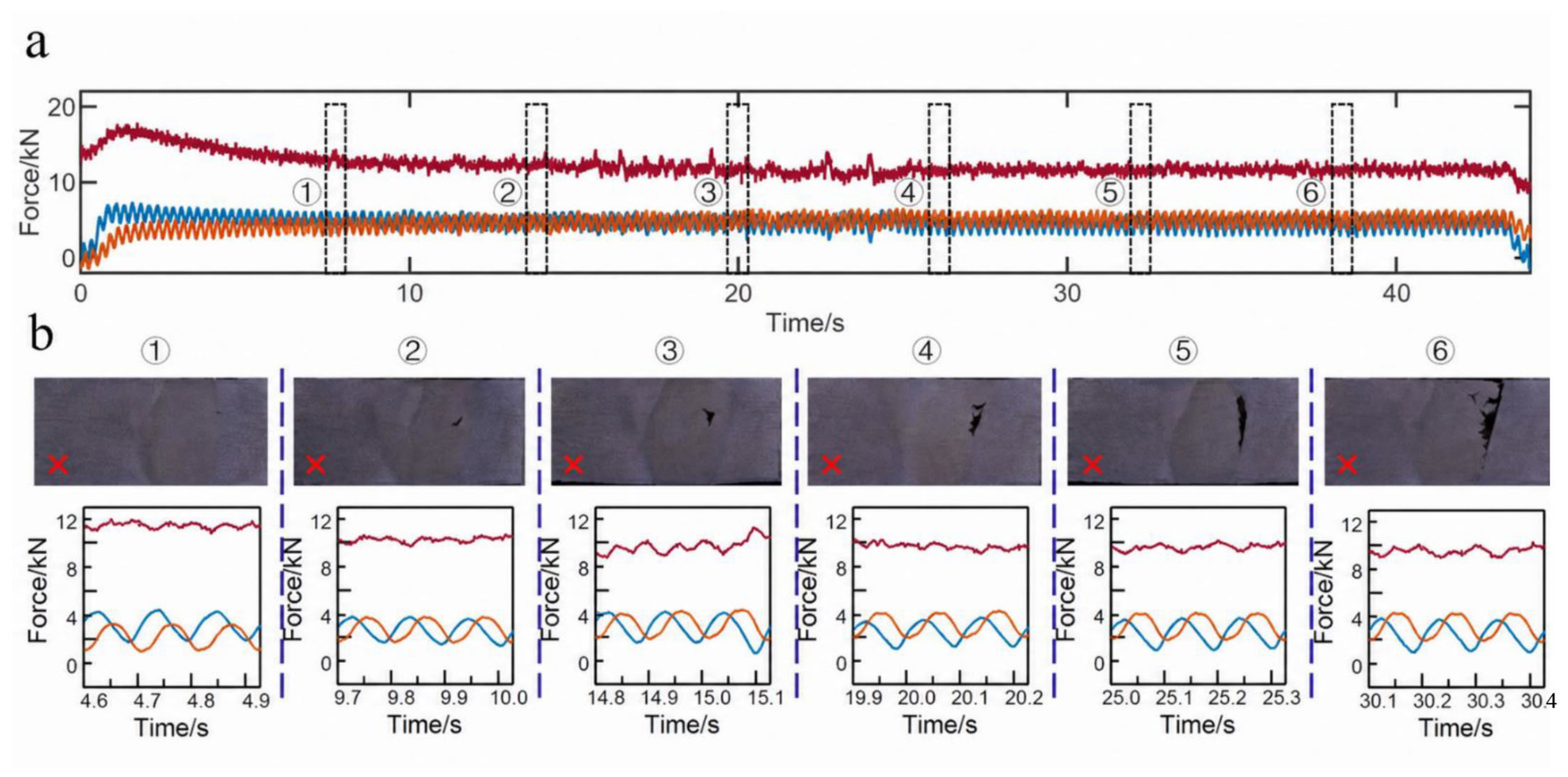
Figure 5 presents the welding force curves for the joint fabricated at 550 rpm and 320 mm/min. During the welding process, Fy steadily increases from 2.5 kN to 3.8 kN, while Fx and Fz remain relatively stable at 3.6 kN and 10.5 kN, respectively. It is observed that void defects form when Fy is lower than Fx. Conversely, when Fy is equal to or greater than Fx, larger tunnel defects are generated in the joints. Furthermore, severe distortions in the waveforms of Fx, Fy, and Fz are closely correlated with the formation of these tunnel defects. Compared with the force signals in Figure 3b and Figure 4b, this defective joint exhibits a noticeable reduction in Fz, severe waveform distortions in all three force components, and an increasing trend in Fy.
The above-mentioned results reveal that the defects in the joints can be reflected directly by the variations in the values and waveforms of the force signals. The increase in Fy, along with the waveform distortions in Fx, Fy, and Fz, is found to be the most apparent characteristic of defects in the joints. As more welding cases are analyzed, the welding force responses associated with defects can become diversified and coupled with each other.

3.2. Force Features for Defect Detection

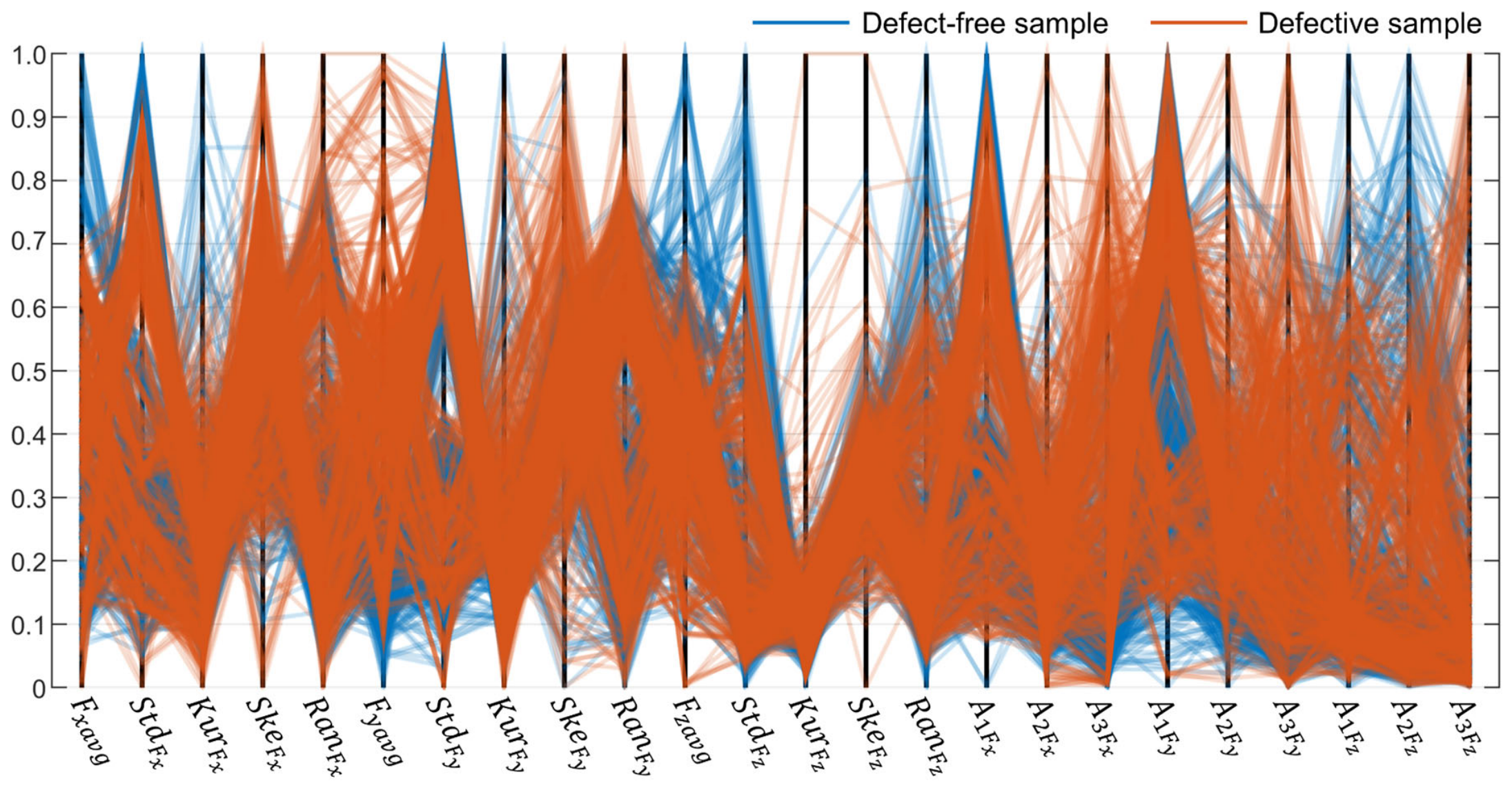
Figure 6 illustrates the correlations between normalized force features and defects across the 724 datasets, where blue and orange lines denote defect-free and defective samples, respectively. As shown in the figure, the distributions of the two sample groups are highly overlapping, without a distinct demarcation between them. This indicates that these features alone cannot directly classify defect-free and defective samples. Nevertheless, it is worth noting that several features show a strong correlation with welding quality within certain ranges. For instance, samples are predominantly defect-free when Fxavg, Fzavg, and StdFz exceed 0.7, and A2Fz surpasses 0.8. Additionally, the occurrence of defects is closely responsible for Fyavg > 0.6 and A3Fx > 0.5. These findings suggest that while specific force features can effectively detect defects within a subset of samples, they are insufficient to yield accurate predictions for the entire dataset of 724 samples.
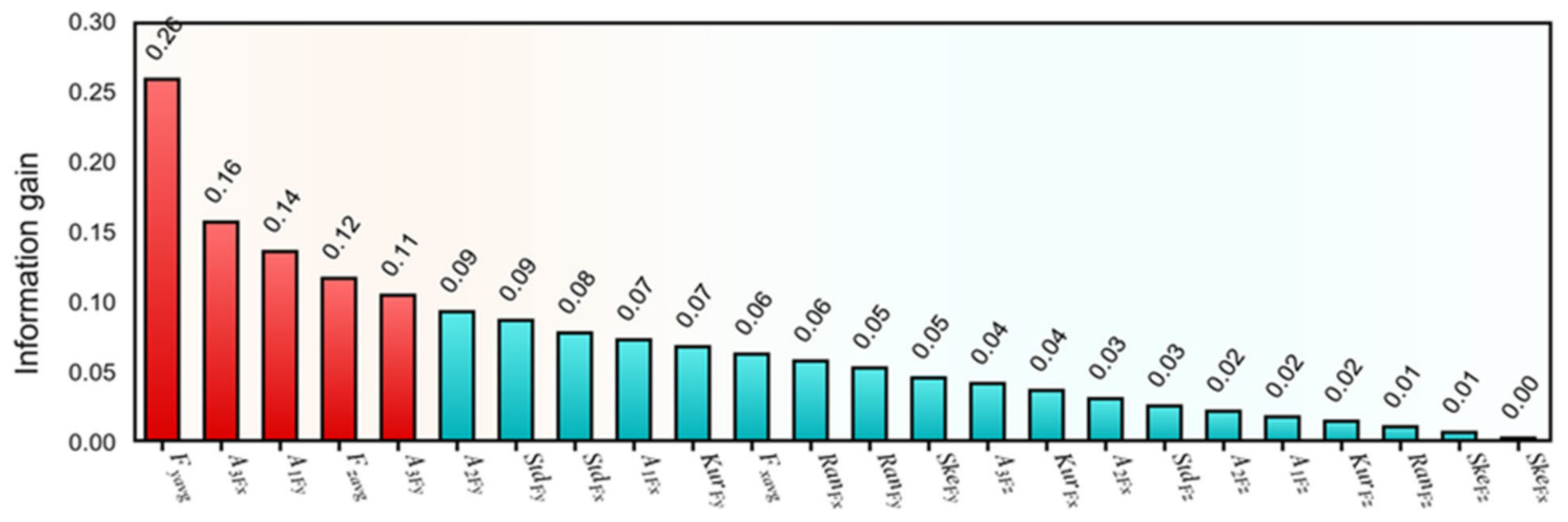
To better understand the correlations between force features and defects, the information gain (IG) values of the force features across the 724 samples were calculated and ranked, as presented in Figure 7. It was observed that Fyavg exhibits the highest correlation with defects, indicating that the average force in the y-direction plays a crucial role in the defect formation process. Subsequently, the three frequency-domain features, namely A3Fx, A1Fy, and A3Fy, extracted from the periodic waveforms of Fx and Fy were found to be relatively less influential on defect formation. In addition, Fzavg ranks fifth in the feature importance hierarchy, while the remaining features derived from Fz occupy the bottom of the list. Clearly, features from Fy demonstrate the strongest correlation with defects, followed by those from Fx and Fz.
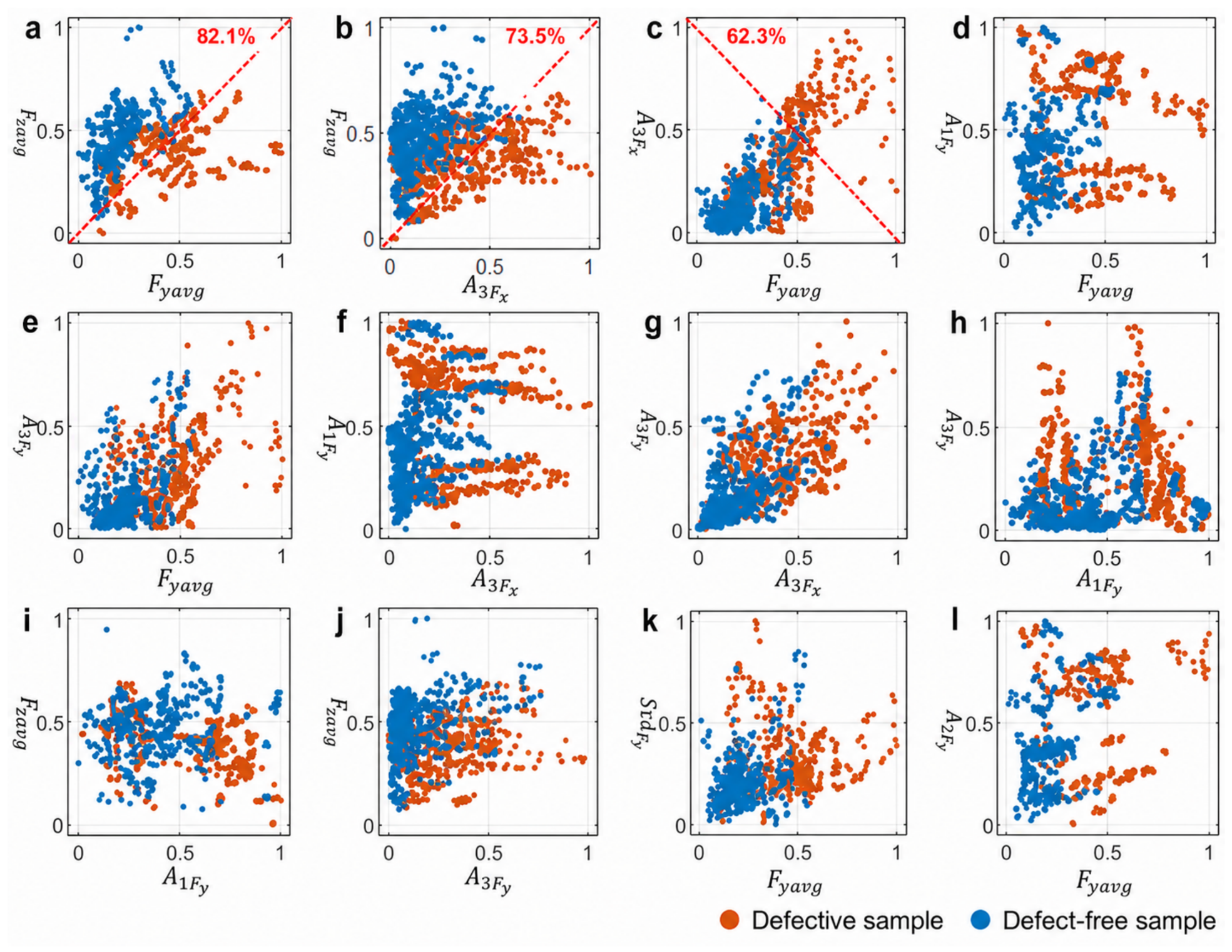
The five most important features ( F y a v g , A 3 F x , A 1 F y , A 3 F y and F z a v g ) were chosen and combined with each other to further classify defect-free and defective samples. Twelve sets of classification results are shown in Figure 8. As shown in Figure 8a, the defective and defect-free samples were mainly distributed in the upper-right and lower-left corners, respectively. The diagonal line ( F y a v g + A 3 F y = 1) was drawn to classify the defect-free and defective samples with an accuracy of 62.3%. In addition, the accuracy of the diagonal lines in Figure 8d,g ( F y a v g = F z a v g ; A 3 F y = F z a v g ) reaches 82.1% and 73.5%. The samples in the remaining figures distributed randomly, indicating that these combinations of force features cannot detect defects. Based on the results in Figure 6, Figure 7 and Figure 8, the relation between the force features and defects is nonlinear. It is hard to extract a single force feature to detect defects because the abundant samples considered more welding conditions than ever.

3.3. Machine Learning for Defect Detection

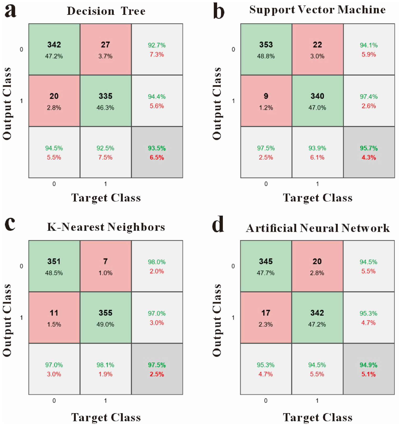
Force features were used to construct machine learning models to detect the defects using four classification algorithms. In addition, class 1 represented the defective samples, while class 0 represented the defect-free samples. The confusion matrices consisting of the correct and incorrect predictions for these four machine learning models are shown in Figure 9. As shown in Figure 9a, the DT model is composed of 677 correct predictions and 47 incorrect predictions, and the accuracy for defect detection reaches 93.5%. The results obtained using the SVM, KNN, and ANN algorithms for defect detection are shown in Figure 9b–d, with accuracies of 95.7%, 97.5% and 94.9%, respectively. The sensitivity and specificity of the four methods are also summarized in Figure 9, which corresponds to the complete dataset.
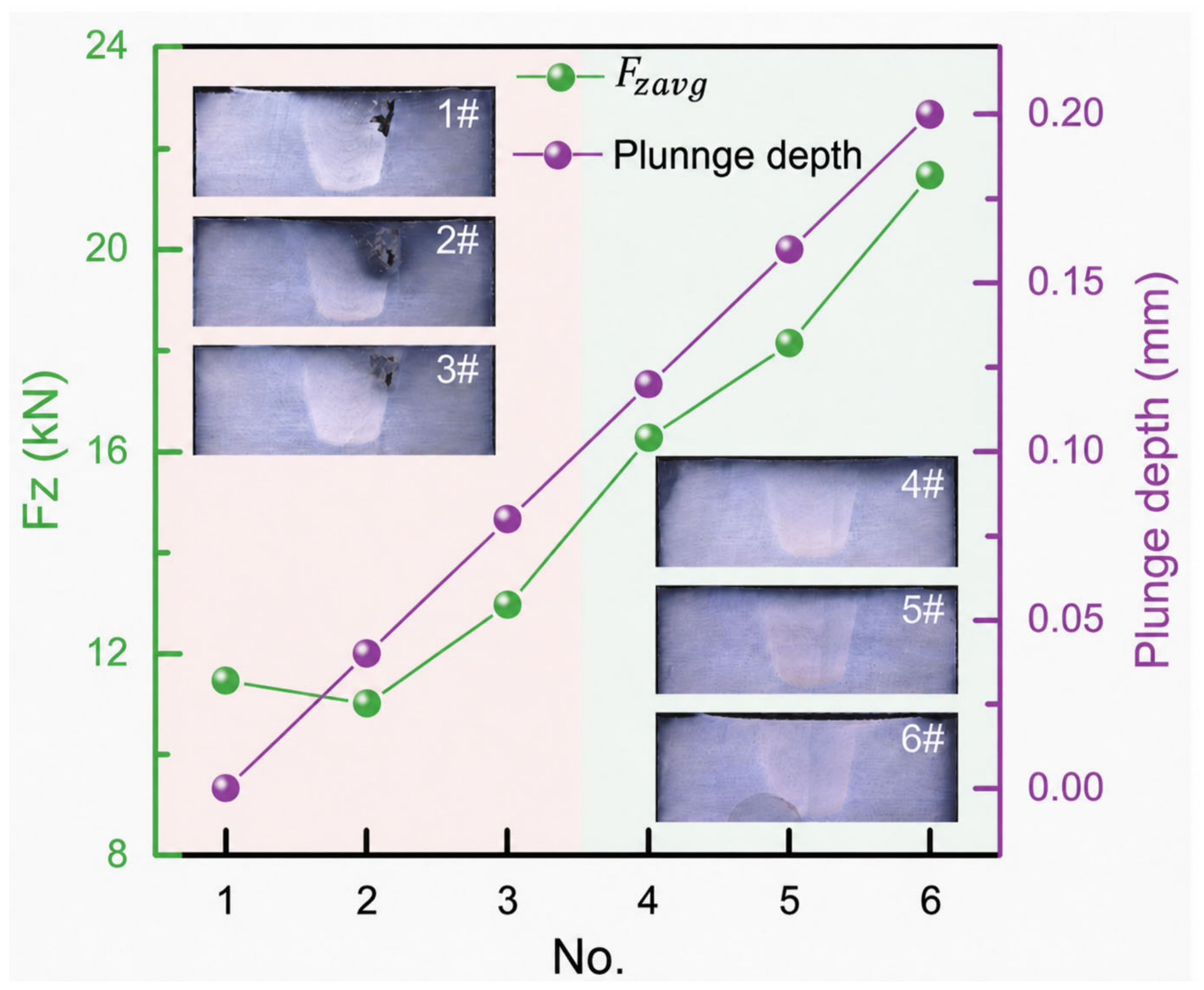
As shown in Figure 10, the average plunge force (Fzavg) generally increased with increasing plunge depth at a constant rotation speed of 600 rpm and traverse speed of 240 mm/min. At relatively low plunge depths, insufficient axial force resulted in inadequate material consolidation, leading to visible internal defects in the joint cross-sections. When the plunge depth increased from 0.12 to 0.20 mm, Fzavg increased substantially and defect-free cross-sections were obtained. These results demonstrate that, within the investigated range, an appropriate increase in plunge depth and Fzavg enhances the forging action of the shoulder and promotes the formation of sound joints.

3.4. Pin-Breaking Experimentation

The three-dimensional force measured before pin fracture is jointly generated by the shoulder and the stirring pin acting on the weld material. The three-dimensional force measured after the fracture of the stirring pin is generated by the shoulder acting on the weld surface. The reduction in the three-dimensional force before and after pin fracture corresponds to the force exerted by the stirring pin on the weld material. Therefore, based on the change in the three-dimensional force before and after pin fracture, the respective proportions of the force contributed by the shoulder and the stirring pin were calculated.
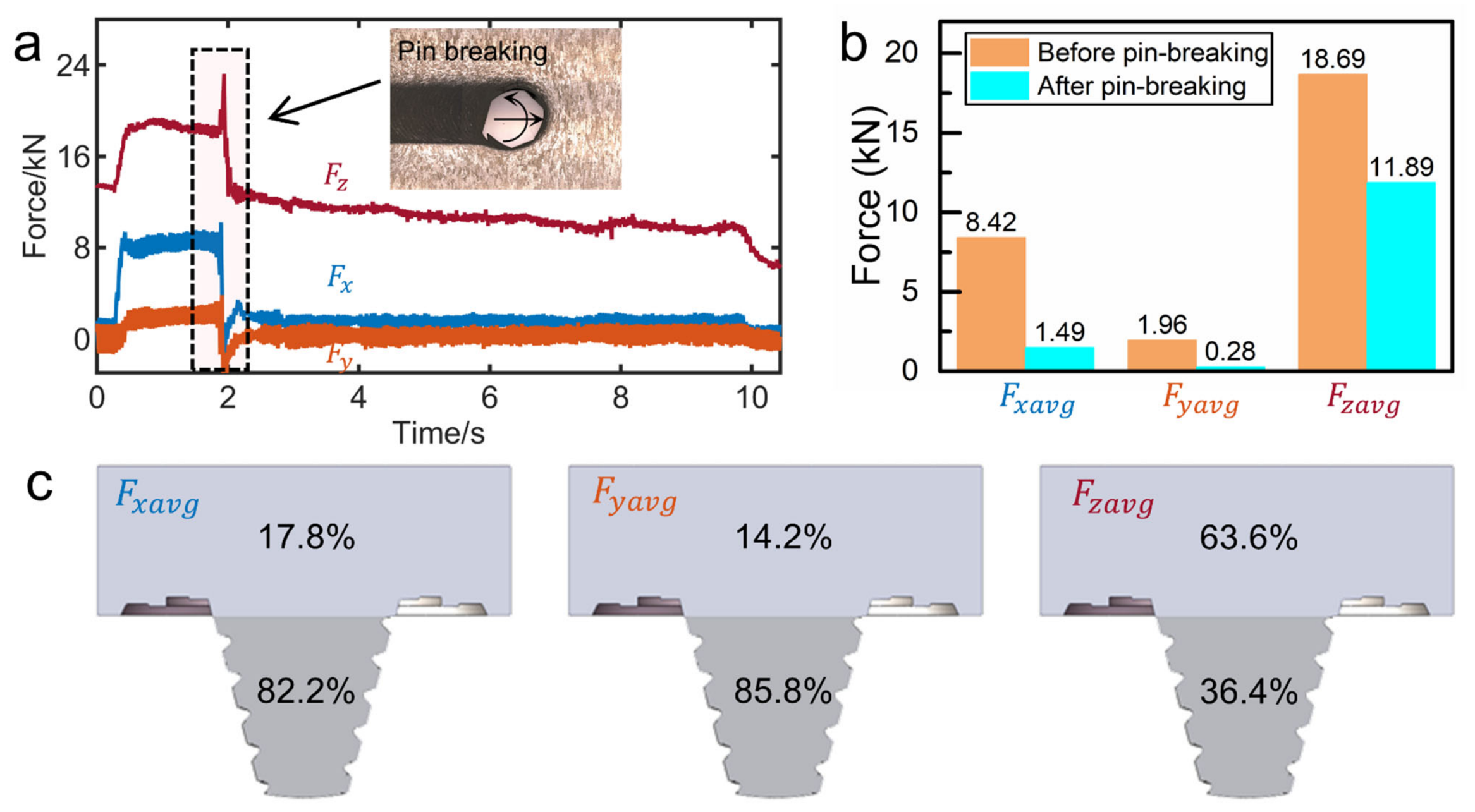
A pin-breaking experiment was conducted to quantitatively investigate the contributions of the shoulder and pin to the welding forces. Considering that the collected force characteristic signals are composed of the force characteristics of different parts of the mixing head, namely the mixing pin and the shaft shoulder, when the mixing pin breaks, the force signal collected is that of the shaft shoulder. As shown in Figure 11a, the pin was intentionally fractured during the welding process, and the resulting variations in welding forces before and after this event were recorded. As illustrated in Figure 11b, prior to pin fracture, the welding forces were generated by the synergistic stirring action of both the shoulder and the pin. Once the pin fractured, the welding forces were exclusively attributed to the shoulder’s extrusion action. Consequently, the observed variations in the force signals are primarily attributed to the loss of the pin’s stirring contribution.
As shown in Figure 11c, the proportions of F x , F y and F z resulting from the shoulder and pin action were calculated. The results quantitatively demonstrate that 82.2% of F x and 85.8% of F y are caused by the stirring action of the pin, while 63.6% of F z is due to the pressure from the shoulder. Therefore, the traverse force ( F x ) and lateral force ( F y ) mainly originate from the stirring action of the pin, while the plunge force ( F z ) is primarily caused by the compression action from the shoulder.

4. Discussion

The results obtained in this study suggest that the force features can help to achieve defect detection in FSW. Defect detection by comparing F y a v g and F z a v g directly has an accuracy of 80.3% for the 724 datasets, while machine learning techniques with force features as input can predict defects with the highest accuracy of 98.0%. A fundamental understanding of the causes of the welding force is necessary to explain the high contributions of welding force in defect detection.
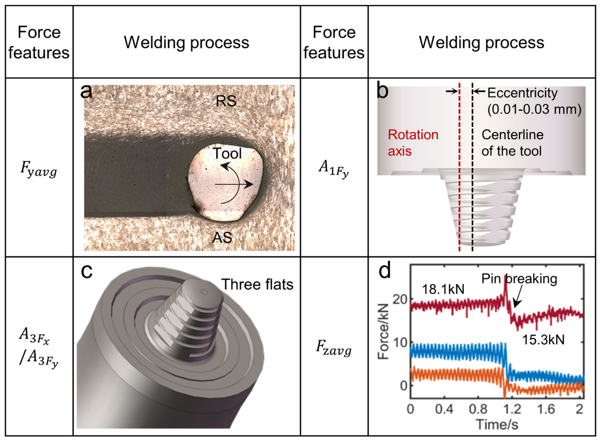
The top five important features are Y a v g , X 3 r d , Y 1 s t , Y 3 r d and Z a v g , indicating that the causes of these features can reveal corresponding abnormal material flow behavior and defect formation processes. The measured F y is the resultant force acting on the plasticized material perpendicular to the welding direction. Previous investigations state that F y has the least influence on the weld quality and little attention is focused on F y [9,11]. In contrast, Y a v g shows the best identification for defects among the twenty-four features. The plasticized material was driven to rotate around the probe along the tool rotation direction, forming the material flow zone [23]. Figure 12a indicates that a lower F y indicates the direction of the driven force close to the flow direction of the plasticized material in the RS, which is beneficial to sufficient material flow around the tool. However, a higher F y leads to the direction of the driven force perpendicular to the welding direction, making the plasticized material compressed and deposited in the RS instead of rotating with the tool. Therefore, Y a v g can be used for detecting defects due to its ability to reveal the direction of the driven force and corresponding material flow.
The first harmonic represents the periodic oscillation characteristic of the welding force, which results from the eccentric motion of the tool [24,25]. Figure 12b illustrates the eccentric distance between the tool’s centerline and rotation axis, and the eccentricity is inherent in typical friction stir welds. Large oscillations of the tool can promote material flow more than one revolution, while lower oscillations result in the material flow for less than one revolution and the defect occurs in the AS due to the low fluidity of materials [26,27]. Furthermore, the periodic first harmonic can reflect periodic material extrusion and flow around the tool influenced by the eccentric oscillation magnitude [12]. The above factors contribute to the high importance of Y 1 s t for defect identification.
As shown in Figure 12c, three flats are designed to promote material flow by improving the dynamic orbit (a ratio between the static volume and dynamic volume which can decide the flow path of the plasticized material around the tool) and generating a pulsating stirring action in the flowing material [28,29]. The cause of the third harmonic of the welding force correlates closely with the three flats because the frequency of the third harmonic was the same as the rotation frequency of the three flats. For defective joints, Frank et al. proposed a hypothesis that when the tool enters the voided region, less material is present to constrain the three flats and reduce the contact force. In this condition, the third harmonic occurs from the distorted welding force [24]. Hence, Y 3 r d and X 3 r d can be used to identify defects in the joints when the tool has three flats.
Figure 12d showed the welding force for the joint with a broken pin. As shown in Figure 12d, F z has a slight reduction from 18.1 kN to 15.3 kN after pin breakage, which indicates that F z results mainly from the interaction between the shoulder and workpiece. The compression and friction between the shoulder and workpiece provide friction heat for the welding process. Furthermore, a lack of forging force in the shoulder means that it cannot move the material from the shoulder-affected zone to the pin-affected zone, resulting in volumetric defects in the joint [30]. In contrast, larger F z leads to excessive frictional heat and defects on the surface, producing defects on the surface of the joints. Hence, only a proper F z can produce defect-free joint.
Although the causes of the top five features and their influences on material flow were discussed, further investigations are required to figure out how these features reveal the defect formation mechanisms based on experimental and simulation results. For example, the effect of three flats on the transient material flow and deposition process during one rotation of the tool with an eccentric motion has not been fully understood. However, the direct interaction between the welding tool and workpiece leads to a welding force that can capture most material flow information during the welding process. As a proven technique, the machine learning technique can acquire hidden relationships from empirical data and provide a promising way for defect detection based on the welding force in FSW.
In FSW, both porosity and tunnel defects result from inadequate material flow and deposition, driven by the discontinuous interaction between the tool and the workpiece. This erratic interaction can be captured by force sensors and is subsequently reflected in the welding force signals, thereby establishing the physical foundation for force-based defect identification. Analyses of three representative joints indicate that defects are typically characterized by an elevated Fz and pronounced waveform distortions in Fx and Fy. These distortions are primarily attributed to high-amplitude third-harmonic components [12]. Frank et al. [24] further elucidated that such distortions in the crests and troughs of the force signals stem from the loss of contact between the three-flatted probe and the surrounding material due to local material absence. This physical interpretation of the welding process and the underlying causes of force variations significantly enhance the interpretability of the machine learning results.
Although the critical role of Fyavg in material flow and defect formation is acknowledged, relying solely on this single feature makes it challenging to accurately identify defects across the 724 samples fabricated under diverse welding parameters. In this study, porosity and tunnel defects were observed in both the shoulder-affected zone and the stir zone. These defects originate from multiple factors, including inadequate or excessive shoulder pressure, inhomogeneous frictional heat input around the tool, and improper welding parameters (e.g., low rotation speeds or high traverse speeds). The multi-mechanism nature of defect formation renders the force responses to defects highly complicated and variable. This complexity explains why twenty-four statistical features were extracted from the force signals and utilized as inputs for the machine learning models in this investigation.

5. Conclusions

An approach for defect detection in FSW based on the welding force with machine learning algorithms is introduced in this work. The main conclusions drawn are as follows:
(1)
The characteristics of the welding forces have high correlations with defects in the FSW joints, such as the increase in F y , decrease in F z and waveform distortions in F x , F y and F z .
(2)
Defect detection based on F y a v g and F z a v g has an accuracy of 82.1% for the 724 datasets. In addition, the accuracy of the DT, KNN, SVM and ANN models for defect detection with the force features as input reached 93.5%, 95.7%, 97.5% and 94.9%, respectively. The decision process of the DT model reveals that F y a v g has the highest importance in defect formation.
(3)
F x and F y result mainly from the extrusion and shear action between the probe and workpiece due to the traverse and rotation motions of the tool. F z is mainly caused by the compression action from the shoulder. The top five important features from F x , F y and F z in defect formation contain F y a v g , A 3 F x , A 1 F y , A 3 F y and F z a v g .

Author Contributions

Conceptualization, W.Z.; Methodology, M.Z.; Software, M.Z.; Formal analysis, J.Z.; Investigation, M.Z., J.Z. and W.Z.; Data curation, J.Z. and W.Z.; Writing—original draft, J.Z. and W.Z.; Writing—review & editing, M.Z. All authors have read and agreed to the published version of the manuscript.

Funding

This research was funded by National Natural Science Foundation of China, grant number 52505420 and the Natural Science Foundation of Tianjin, grant number 24JCQNJC01790.

Data Availability Statement

The original contributions presented in this study are included in the article. Further inquiries can be directed to the corresponding author.

Acknowledgments

This research was funded by National Natural Science Foundation of China, grant number 52505420 and the Natural Science Foundation of Tianjin, grant number 24JCQNJC01790. The authors would like to express the deepest gratitude to Wei Guan for his valuable guidance in this work.

Conflicts of Interest

The authors declare no conflicts of interest.

References

  1. Mishra, R.S.; Ma, Z.Y. Friction Stir Welding and Processing. Mater. Sci. Eng. R 2005, 50, 1–78. [Google Scholar] [CrossRef] [Scilit]
  2. Meng, X.; Huang, Y.; Cao, J.; Shen, J.; dos Santos, J.F. Recent progress on control strategies for inherent issues in friction stir welding. Prog. Mater. Sci. 2021, 115, 100706. [Google Scholar] [CrossRef] [Scilit]
  3. Chen, G.; Zhang, S.; Zhu, Y.; Yang, C.; Shi, Q. Thermo-mechanical Analysis of Friction Stir Welding: A Review on Recent Advances. Acta Metall. Sin. (Engl. Lett.) 2019, 33, 3–12. [Google Scholar] [CrossRef] [Scilit]
  4. Aziz, S.B.; Dewan, M.W.; Huggett, D.J.; Wahab, M.A.; Okeil, A.M.; Liao, T.W. A fully coupled thermomechanical model of friction stir welding (FSW) and numerical studies on process parameters of lightweight aluminum alloy joints. Acta Metall. Sin. (Engl. Lett.) 2017, 31, 1–18. [Google Scholar] [CrossRef] [Scilit]
  5. Li, B.; Shen, Y.; Hu, W. The study on defects in aluminum 2219-T6 thick butt friction stir welds with the application of multiple non-destructive testing methods. Mater. Des. 2011, 32, 2073–2084. [Google Scholar] [CrossRef] [Scilit]
  6. Kadian, A.K.; Biswas, P. Effect of tool pin profile on the material flow characteristics of AA6061. J. Manuf. Process. 2017, 26, 382–392. [Google Scholar] [CrossRef] [Scilit]
  7. Zhao, Y.; Han, J.; Domblesky, J.P.; Yang, Z.; Li, Z.; Liu, X. Investigation of void formation in friction stir welding of 7N01 aluminum alloy. J. Manuf. Process. 2019, 37, 139–149. [Google Scholar] [CrossRef] [Scilit]
  8. Shrivastava, A.; Pfefferkorn, F.E.; Duffie, N.A.; Ferrier, N.J.; Smith, C.B.; Malukhin, K.; Zinn, M. Physics-based process model approach for detecting discontinuity during friction stir welding. Int. J. Adv. Manuf. Technol. 2015, 79, 605–614. [Google Scholar] [CrossRef] [Scilit]
  9. Eslami, S.; Mourão, L.; Viriato, N.; Tavares, P.J.; Moreira, P.M.G.P. Multi-axis force measurements of polymer friction stir welding. J. Mater. Process. Technol. 2018, 256, 51–56. [Google Scholar] [CrossRef] [Scilit]
  10. Das, B.; Pal, S.; Bag, S. Design and development of force and torque measurement setup for real time monitoring of friction stir welding process. Measurement 2017, 103, 186–198. [Google Scholar] [CrossRef] [Scilit]
  11. Das, B.; Pal, S.; Bag, S. Weld defect identification in friction stir welding using power spectral density. In Proceedings of the IOP Conference Series: Materials Science and Engineering, Dubai, United Arab Emirates, 28–29 November 2017; Volume 346, p. 012049. [Google Scholar]
  12. Guan, W.; Li, D.; Cui, L.; Wang, D.; Wu, S.; Kang, S.; Wang, J.; Mao, L.; Zheng, X. Detection of tunnel defects in friction stir welded aluminum alloy joints based on the in-situ force signal. J. Manuf. Process. 2021, 71, 1–11. [Google Scholar] [CrossRef] [Scilit]
  13. Shrivastava, A.; Zinn, M.; Duffie, N.A.; Ferrier, N.J.; Smith, C.B.; Pfefferkorn, F.E. Force measurement-based discontinuity detection during friction stir welding. J. Manuf. Process. 2017, 26, 113–121. [Google Scholar] [CrossRef] [Scilit]
  14. Kumari, S.; Jain, R.; Kumar, U.; Yadav, I.; Ranjan, N.; Kumari, K.; Kesharwani, R.K.; Kumar, S.; Pal, S.; Pal, S.K.; et al. Defect identification in friction stir welding using continuous wavelet transform. J. Intell. Manuf. 2016, 30, 483–494. [Google Scholar] [CrossRef] [Scilit]
  15. Kumar, U.; Yadav, I.; Kumari, S.; Kumari, K.; Ranjan, N.; Kesharwani, R.K.; Jain, R.; Kumar, S.; Pal, S.; Chakravarty, D.; et al. Defect identification in friction stir welding using discrete wavelet analysis. Adv. Eng. Softw. 2015, 85, 43–50. [Google Scholar] [CrossRef] [Scilit]
  16. Das, B.; Pal, S.; Bag, S. Weld quality prediction in friction stir welding using wavelet analysis. Int. J. Adv. Manuf. Technol. 2016, 89, 711–725. [Google Scholar] [CrossRef] [Scilit]
  17. Dehabadi, V.M.; Ghorbanpour, S.; Azimi, G. Application of artificial neural network to predict Vickers microhardness of AA6061 friction stir welded sheets. J. Cent. South Univ. 2016, 23, 2146–2155. [Google Scholar] [CrossRef] [Scilit]
  18. Senapati, N.P.; Panda, D.K.; Bhoi, R.K. Prediction of multiple characteristics of Friction-Stir welded joints by Levenberg–Marquardt algorithm based artificial neural network. Mater. Today Proc. 2020, 27, 871–876. [Google Scholar]
  19. Sudhagar, S.; Sakthivel, M.; Ganeshkumar, P. Monitoring of friction stir welding based on vision system coupled with Machine learning algorithm. Measurement 2019, 144, 135–143. [Google Scholar] [CrossRef] [Scilit]
  20. Dhanraj, J.A.; Lingampalli, B.; Prabhakar, M.; Sivakumar, A.; Krishnamurthy, B.; Ramanathan, K.C. A credal decision tree classifier approach for surface condition monitoring of friction stir weldment through vibration patterns. Mater. Today Proc. 2021, 46, 1127–1133. [Google Scholar] [CrossRef] [Scilit]
  21. Du, Y.; Mukherjee, T.; DebRoy, T. Conditions for void formation in friction stir welding from machine learning. npj Comput. Mater. 2019, 5, 68. [Google Scholar] [CrossRef] [Scilit]
  22. Du, Y.; Mukherjee, T.; Mitra, P.; DebRoy, T. Machine learning based hierarchy of causative variables for tool failure in friction stir welding. Acta Mater. 2020, 192, 67–77. [Google Scholar] [CrossRef] [Scilit]
  23. Liu, F.C.; Nelson, T.W. In-situ material flow pattern around probe during friction stir welding of austenitic stainless steel. Mater. Des. 2016, 110, 354–364. [Google Scholar] [CrossRef] [Scilit]
  24. Franke, S.R.D.; Zinn, M.; Pfefferkorn, F.E. Understanding process force transients with application towards defect detection during friction stir welding of aluminum alloys. J. Manuf. Process. 2020, 54, 251–261. [Google Scholar] [CrossRef] [Scilit]
  25. Zaeh, M.F.; Gebhard, P. Dynamical behaviour of machine tools during friction stir welding. Prod. Eng. 2010, 4, 615–624. [Google Scholar] [CrossRef] [Scilit]
  26. Chen, Y.; Wang, H.; Wang, X.; Ding, H.; Zhao, J.; Zhang, F.; Ren, Z. Influence of tool pin eccentricity on microstructural evolution and mechanical properties of friction stir processed Al-5052 alloy. Mater. Sci. Eng. A 2019, 739, 272–276. [Google Scholar] [CrossRef] [Scilit]
  27. Mao, Y.; Ke, L.; Liu, F.; Liu, Q.; Huang, C.; Xing, L. Effect of tool pin eccentricity on microstructure and mechanical properties in friction stir welded 7075 aluminum alloy thick plate. Mater. Des. (1980–2015) 2014, 62, 334–343. [Google Scholar] [CrossRef] [Scilit]
  28. Shah, L.H.; Walbridge, S.; Gerlich, A. Tool eccentricity in friction stir welding: A comprehensive review. Sci. Technol. Weld. Join. 2019, 24, 566–578. [Google Scholar] [CrossRef] [Scilit]
  29. Su, H.; Wu, C. Numerical simulation for the optimization of polygonal pin profiles in friction stir welding of aluminum. Acta Metall. Sin. (Engl. Lett.) 2021, 34, 1065–1078. [Google Scholar] [CrossRef] [Scilit]
  30. Liu, X.C.; Wu, C.S. Elimination of tunnel defect in ultrasonic vibration enhanced friction stir welding. Mater. Des. 2016, 90, 350–358. [Google Scholar] [CrossRef] [Scilit]
Figure 1. A schematic of welding force driven machine learning for defect detection in FSW.
Crystals 16 00573 g001
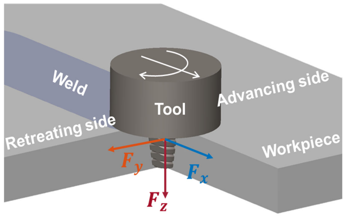
Figure 2. Schematic diagram of the welding force in the FSW processing.
Crystals 16 00573 g002
Figure 3. Welding force and cross-sections for FSW joints welded with 550 rpm 160 mm/min (green ticks refer to acceptable-quality welds, red lines indicate Fz, blue lines indicate Fx, and orange lines indicate Fy): (a) welding force signals during the welding process; (b) welding force signals at the locations of six samples.
Crystals 16 00573 g003
Figure 4. Welding force and cross-sections for FSW joints welded with 550 rpm and 240 mm/min (green ticks refer to acceptable-quality welds, and red crosses refer to unacceptable-quality welds, red lines indicate Fz, blue lines indicate Fx, and orange lines indicate Fy): (a) welding force signals during the welding process; (b) welding force signals at the locations of six samples.
Crystals 16 00573 g004
Figure 5. Welding force and cross-sections for FSW joints welded with 550 rpm and 320 mm/min (red crosses refer to unacceptable-quality welds, red lines indicate Fz, blue lines indicate Fx, and orange lines indicate Fy): (a) welding force signals during the welding process; (b) welding force signals at the locations of six samples.
Crystals 16 00573 g005
Figure 6. Parallel coordinate plot of defect distribution for the twenty-four force features.
Crystals 16 00573 g006
Figure 7. The IG ranking of the twenty-four force features for the 724 datasets.
Crystals 16 00573 g007
Figure 8. The distribution of defect-free and defective samples based on the paired features from F y a v g , A 3 F x , A 1 F y , A 3 F y and F z a v g for the 724 datasets.
Crystals 16 00573 g008
Figure 9. Confusion matrices of four machine learning algorithms in the adjusted 362 + 362-case evaluation set. Rows indicate output class and columns indicate target class. (a) Decision Tree, (b) Support Vector Machine, (c) K-Nearest Neighbors, and (d) Artificial Neural Network.
Crystals 16 00573 g009
Figure 10. Relationship between the average plunge force, plunge depth, and cross-sectional defect morphology of joints welded at 600 rpm and 240 mm/min.
Crystals 16 00573 g010
Figure 11. The welding force for the pin-breaking experiment: (a) the pin-breaking process; (b) the variations in F x   F y   a n d   F z before and after the pin-breaking moment; (c) the proportion of welding forces driven by the shoulder and pin.
Crystals 16 00573 g011
Figure 12. The relationships between the force characteristics and welding behaviors: (a) Fy-material flow around the tool probe; (b) A1Fy-eccentric distance of the tool; (c) A3Fx/A3Fy-three flats at the tool probe; (d) Fzavg-the compression action of the tool shoulder.
Crystals 16 00573 g012
Table 1. Key indicators of the three-axis force measuring system.
Load Rating/kNSensitivity/‰Repeatability Error/‰Hysteresis Error/‰
F x 401.001.00.15
F y 401.00
F z 600.90
Table 2. The definitions, formulas and abbreviations of the force features.
FeatureFormulaAbbreviation
Average   of   F x ,   F y   and   F z F a v g = i = 1 n f i n F x a v g   F y a v g   F z a v g
Range   of   F x ,   F y   and   F z R a n = F m a x F m i n R a n F x   R a n F y   R a n F z
Standard   deviation   of   F x ,   F y   and   F z S t d = i = 1 n ( f i F a v g ) 2 n S t d F x   S t d F y   S t d F z
Skewness   of   F x ,   F y   and   F z S k e = 1 n i = 1 n ( f i F a v g ) 3 ( 1 n i = 1 n ( f i F a v g ) 2 ) 3 2 S k e F x   S k e F y   S k e F z
Kurtosis   of   F x ,   F y     and   F z K u r = 1 n i = 1 n ( f i F a v g ) 4 ( 1 n i = 1 n ( f i F a v g ) 2 ) 2 K u r F x   K u r F y   K u r F z
The   1 st   harmonic   amplitude   of   F x ,   F y   and   F z A 1 = A f 0 A f = F F T f t A 1 F x   A 1 F y   A 1 F z
The   2 nd   harmonic   amplitude   of   F x ,   F y   and   F z A 2 = A 2 f 0 A 2 F x   A 2 F y   A 2 F z
The   3 rd   harmonic   amplitude   of   F x ,   F y   and   F z A 3 = A 3 f 0 A 3 F x   A 3 F y   A 3 F z
Table 3. Description of the machine learning models.
AlgorithmRecommended Reproducibility Configuration
Decision Treecriterion = gini; max_depth = 8; min_samples_split = 10; min_samples_leaf = 4; ccp_alpha = 0.001
Support Vector Machinekernel = rbf; C = 10.0; gamma = scale; class_weight = balanced; probability = True
K-Nearest Neighborsn_neighbors = 7; weights = distance; algorithm = auto; p = 2; metric = minkowski
Artificial Neural Networkhidden_layers = [64, 32]; optimizer = Adam; learning_rate = 0.001; batch_size = 32; dropout = 0.20
Disclaimer/Publisher’s Note: The statements, opinions and data contained in all publications are solely those of the individual author(s) and contributor(s) and not of MDPI and/or the editor(s). MDPI and/or the editor(s) disclaim responsibility for any injury to people or property resulting from any ideas, methods, instructions or products referred to in the content.