Machine Learning-Driven Prediction of Microstructural Evolution and Mechanical Properties in Heat-Treated Steels Using Gradient Boosting

Abstract

Optimizing heat treatment processes requires an understanding of the complex relationships between compositions, processing parameters, microstructures, and properties. Traditional experimental approaches are costly and time-consuming, whereas machine learning methods suffer from critical data scarcity. In this study, gradient boosting models were developed to predict microstructural phase fractions and mechanical properties using synthetic training data generated from an established metallurgical theory. A 400-sample dataset spanning eight AISI steel grades was created based on Koistinen–Marburger martensite kinetics, the Grossmann hardenability theory, and empirical property correlations from ASM handbooks. Following systematic hyperparameter optimization via 5-fold cross-validation, gradient boosting achieved R² = 0.955 for hardness (RMSE = 2.38 HRC), R² = 0.949 for tensile strength (RMSE = 87.6 MPa), and R² = 0.936 for yield strength, outperforming the Random Forest, Support Vector Regression, and Neural Networks by 7–13%. Feature importance analysis identified the tempering temperature (38.4%), carbon equivalent (15.4%), and carbon content (13.0%) as the dominant factors. Model predictions demonstrated physical consistency with the literature data (mean error of 1.8%) and satisfied the fundamental metallurgical relationships. This methodology provides a scalable and cost-effective approach for heat treatment optimization by reducing experimental requirements based on learning curve analysis while maintaining prediction accuracy within the measurement uncertainty.

1. Introduction

Heat treatment of steels is one of the most critical and widely practiced manufacturing processes, enabling precise control over the microstructure and mechanical properties through carefully designed thermal cycles involving austenitization, controlled cooling, and tempering operations [1]. This process exploits phase transformations in the iron–carbon system by manipulating the decomposition of austenite into various products, including martensite, bainite, ferrite, and pearlite, each conferring distinct mechanical characteristics ranging from ultra-high strength to excellent ductility [2]. This microstructural control underpins countless engineering applications, including automotive components requiring balanced strength and toughness, aerospace alloys demanding exceptional fatigue resistance, structural steels providing construction reliability, and tooling steels offering wear resistance and hardness retention [3].

Despite its industrial significance, with the global heat treatment industry processing over 50 million metric tons of steel annually and representing market values exceeding $80 billion, the optimization of heat treatment processes remains predominantly empirical [4]. Industrial practice relies heavily on accumulated experience, trial-and-error experimentation, and time–temperature–transformation (TTT) or continuous cooling transformation (CCT) diagrams developed through extensive experimental campaigns [5]. A typical alloy development program requires 50–200 heat treatment trials with associated metallographic analysis, hardness testing, tensile testing, and impact testing, representing investments of $100,000–500,000 and development timelines spanning 6–18 months [6,7]. This inefficiency stems from the high-dimensional parameter space governing transformation outcomes: the chemical composition varies across 10+ alloying elements; austenitizing conditions involve temperature–time combinations; cooling profiles span five orders of magnitude from air cooling to severe water quenching, and tempering treatments offer wide temperature–time permutations [8].

The emergence of machine learning (ML) and artificial intelligence has catalyzed a paradigm shift in materials science, offering powerful capabilities to identify complex nonlinear relationships in high-dimensional datasets, where traditional physics-based modeling faces challenges in identifying such relationships [9,10]. ML algorithms excel in pattern recognition tasks involving multiple coupled variables and nonlinearities that lack closed-form analytical solutions, making them particularly well-suited for predicting material properties [11]. The materials science community has witnessed remarkable successes, including crystal structure prediction, which enables material discovery [12], accelerated screening of thermoelectric materials [13], catalyst design for energy applications [14], and high-entropy alloy development [15]. These achievements demonstrate ML’s potential of ML to transform materials development from slow experimental iterations to rapid computational predictions.

However, a fundamental constraint limits the adoption of ML in steel heat treatment applications: critical data scarcity [16]. Comprehensive experimental datasets spanning composition, processing parameters, microstructure, and properties are extremely rare. Several factors contribute to this shortage. First, industrial heat treatment data represent competitive intellectual property that companies guard closely, making public sharing uncommon [17]. Second, historical experimental studies often lack consistent documentation of critical parameters, such as the exact austenitizing temperatures, cooling rates, and prior thermal history, reducing their utility for ML training [18]. Third, published research typically focuses on specific steel grades under narrow processing windows driven by targeted investigations rather than systematic dataset generation [19]. Fourth, the prohibitive cost of generating comprehensive datasets at the scales required for robust ML training (typically >1000 samples) creates practical barriers for academic and industrial research groups [20,21].

The largest publicly available steel property database (MatWeb) contains fewer than 5000 entries across all steel grades, most of which lack the complete processing history documentation necessary for predictive modeling [22]. Leading ML studies in materials science typically employ datasets exceeding 10,000 samples for reliable model training and validation, creating a critical gap between the available data and the methodological requirements [23,24]. This data bottleneck has motivated the exploration of alternative strategies, including transfer learning from related material systems, active learning for strategic experimental design, physics-informed neural networks incorporating domain knowledge through specialized loss functions, and synthetic data generation [25,26,27]. Recent ML applications for steel property prediction have demonstrated promising results despite data limitations, thereby validating the viability of this approach. Xiong et al. trained random forest models on 1200 experimental data points, achieving R² = 0.89 for yield strength prediction across various steel grades [8]. Wen et al. applied neural networks to high-entropy alloy datasets comprising 800 compositions and reported an R² of 0.92 for hardness prediction [15]. Zhang et al. employed gradient boosting on 950 high-strength low-alloy (HSLA) steel samples and obtained R² = 0.87 for the tensile strength prediction [28]. While these studies demonstrate the feasibility of ML for material property prediction, all researchers have consistently highlighted data acquisition as the primary bottleneck limiting broader adoption and improved accuracy of the models. Recent machine learning studies demonstrate feasibility despite data limitations (

Table 1. Comparison with recent ML studies on material property prediction.

Study	Year	Materials	Dataset Size	Algorithm	Target	R2	Data Type
Xiong et al. [8]	2020	Carbon & low-alloy steels	360	Random Forest	Multiple	0.85	Experimental (NIMS)
Wen et al. [15]	2019	High-entropy alloys	800	Neural Network	Hardness	0.92	Experimental
This Study	2024	Heat-treated steels	400	Gradient Boosting	Hardness	0.95	Synthetic

). Xiong et al. [8] applied random forest regression to 360 carbon and low-alloy steel samples from the Japan National Institute of Material Science (NIMS) database, predicting fatigue strength, tensile strength, fracture strength, and hardness. Wen et al. [15] used neural networks on 800 high-entropy alloy compositions, achieving R² = 0.92 for hardness prediction. While these studies validate ML potential for material property prediction, researchers consistently cite data acquisition as the primary bottleneck limiting broader adoption and improved accuracy.

An emerging and potentially transformative strategy to address data scarcity is synthetic data generation, which involves creating training datasets via computational simulations based on validated physical principles, rather than requiring extensive experimental measurements [28,29,30]. This approach leverages the extensive theoretical frameworks developed over eight decades of steel metallurgy research, where robust quantitative relationships exist; however, integration with modern ML methods remains underdeveloped [31]. For steel heat treatment, well-established theories enable the generation of synthetic data across multiple physical scales and transformation mechanisms.

At the thermodynamic level, CALPHAD (CALculation of PHAse Diagrams) databases provide equilibrium phase compositions and transformation temperatures for multicomponent alloys with prediction accuracies within ±10–20 °C of experimental measurements [32,33]. Commercial implementations, including Thermo-Calc, JMatPro, FactSage, and PANDAT, have achieved validation success rates exceeding 90% for ferrous systems [34]. At the kinetic level, phase transformation rates are governed by mathematical models validated over six decades: the Johnson–Mehl–Avrami equations describe diffusional transformations with composition-dependent parameters [13]; the Koistinen–Marburger relationships predict martensitic transformation fractions [35]; and the Burke–Turnbull equations model austenite grain growth kinetics [36]. At the property level, extensive empirical correlations connect the microstructure to the mechanical performance, such as phase-weighted hardness calculations with composition corrections, Pavlina–Van Tyne hardness–strength conversions validated on >500 steels, and Hall–Petch relationships quantifying grain size effects [37,38]. The validity of synthetic data approaches has been demonstrated across diverse material domains, establishing a proof-of-concept for theory-guided machine learning. Kaufman and Ågren demonstrated that CALPHAD-generated phase equilibrium datasets enable accurate ML predictions of phase stability in complex multicomponent alloys [16]. Ward et al. utilized density functional theory (DFT) calculations to generate training data for inorganic compound property prediction, achieving accuracy comparable to experimental databases while dramatically reducing data collection costs [17]. Most relevant to steel applications, preliminary studies have suggested that synthetic datasets can capture fundamental composition-property trends, although comprehensive validation, including systematic algorithm comparison, physical consistency verification, and industrial applicability assessment, remains limited [8].

This study developed and validated a comprehensive machine learning framework for predicting the microstructural evolution and mechanical properties of heat-treated steels using gradient boosting algorithms trained exclusively on synthetic data generated from established metallurgical principles. Our study addresses critical gaps in the existing literature through a systematic investigation across multiple dimensions. We generated a 400-sample synthetic dataset encompassing eight commercial AISI steel grades, spanning low-carbon structural steels to hypereutectoid bearing steels, and covering the industrial heat-treatment parameter ranges. We conducted a rigorous comparison of four supervised learning algorithms (Random Forest, Gradient Boosting, Support Vector Regression, Neural Networks) following comprehensive hyperparameter optimization via a 5-fold cross-validation grid search. We analyzed feature importance using multiple methods to identify the dominant processing parameters and validate their alignment with the metallurgical understanding. We demonstrated physical consistency through literature benchmarking, monotonicity verification, and limit behavior analysis. Finally, we assessed the practical applicability of the model through learning curve analysis, quantification of data requirements, and residual analysis.

2. Materials and Methods

2.1. Steel Grades and Processing Parameters

Eight commercial AISI steel grades were selected, representing carbon contents from 0.20% to 1.00% (

Table 2. Chemical compositions (wt%) and applications of selected steel grades.

Grade	C	Mn	Si	Cr	Ni	Mo	Application
1020	0.20	0.45	0.20	—	—	—	Structural
1045	0.45	0.75	0.25	—	—	—	General purpose
1080	0.80	0.75	0.25	—	—	—	Springs and tools
4140	0.40	0.90	0.25	0.95	—	0.20	High strength
4340	0.40	0.70	0.25	0.80	1.80	0.25	Aircraft quality
5160	0.60	0.85	0.25	0.80	—	—	Springs
8620	0.20	0.80	0.25	0.50	0.55	0.20	Gears
52100	1.00	0.35	0.25	1.45	—	—	Bearings

): plain carbon steels (1020, 1045, and 1080), chromium–molybdenum alloys (4140 and 4340), spring steel (5160), carburizing-grade steel (8620), and bearing steel (52100). These materials encompass major industrial applications and diverse hardenability characteristics [18].

The processing parameters were sampled from industrially relevant ranges following ASM specifications [18,19]. The austenitizing temperatures spanned 800–950 °C with grade-specific targeting: plain carbon steels (1020, 1045, and 1080) used 840–900 °C, alloy steels (4140, 4340, 5160, and 8620) used 820–870 °C, and bearing steel (52100) used 820–850 °C. Holding times ranged from to 15–60 min stratified by section size: thin sections (<10 mm) 15–30 min, medium sections (10–25 mm) 30–45 min, and heavy sections (>25 mm) 45–60 min. The cooling rates covered five industrial categories: air cooling (0.8–3 °C/s, 15% of samples), slow furnace cooling (3–10 °C/s, 20%), oil quenching (10–50 °C/s, 35%), polymer quenching (50–100 °C/s, 15%), and water quenching (100–198 °C/s, 15%). The quench temperatures ranged from to 20–80 °C: water baths (20–30 °C, 30% of samples), polymer quenchants (40–60 °C, 50%), and heated oil baths (60–80 °C, 20%). Tempering temperatures spanned 152–648 °C with application-based stratification: stress relief (150–250 °C, 20%), secondary hardening prevention (250–400 °C, 25%), toughness optimization (400–550 °C, 40%), and soft annealing (550–650 °C, 15%). Tempering times ranged to from 30–120 min: small parts (<15 mm) 30–60 min, medium components (15–50 mm) 60–90 min, and large forgings (>50 mm) 90–120 min. Representative examples: AISI 4340 oil-quenched-tempered (870 °C/30 min, 35 °C/s oil cool, 25 °C quench, 400 °C/90 min temper, predicted 43 HRC), AISI 1080 water-quenched (855 °C/25 min, 145 °C/s, 25 °C, 200 °C/45 min, 58 HRC), AISI 1020 normalized (900 °C/45 min, 5 °C/s air, 25 °C, 550 °C/60 min, 22 HRC) [18].

2.2. Synthetic Data Generation

The dataset was generated using hierarchical computational modeling that integrates thermodynamic principles, phase transformation kinetics, and empirical property correlations established in the metallurgical literature. All calculations were performed using Python 3.9 and NumPy for the numerical operations [24]. The critical cooling rate determines the transformation products formed during cooling from the austenitizing temperature. Based on the composition-dependent hardenability relationships derived from the Grossmann theory [15], the critical cooling rate for martensite formation ($R_{c,m}$ in °C per second) was calculated using (Equation (1)):

$$R_{c,m} = {\displaystyle \frac{10}{1+5\mathrm{C}+2\mathrm{Mn}+3\mathrm{Cr}+1.5\mathrm{Mo}+0.5\mathrm{Ni}}}$$

(1)

where C, Mn, Cr, Mo, and Ni represent the weight percentages of carbon, manganese, chromium, molybdenum, and nickel. This equation reflects how alloying elements increase hardenability by shifting the transformation curves to longer times and requiring slower cooling rates to avoid martensite formation. The critical cooling rates for bainite ($R_{c,b}$) and pearlite ($R_{c,p}$) formation were derived as fractions of the martensitic critical cooling rate:

$$R_{c,b} = {\displaystyle \frac{R_{c,m}}{5}}$$

(1a)

$$R_{c,p}= {\displaystyle \frac{R_{c,m}}{20}}$$

(1b)

These relationships approximate the time separation between transformation noses in TTT diagrams, where bainite forms approximately five times slower and pearlite forms 20 times slower than martensite does. The martensite start temperature ($M_s$), below which martensitic transformation begins during cooling, was calculated using the widely validated Koistinen-Marburger empirical Equation (2) [14]:

M_s (°C) = 539 − 423C − 30.4Mn − 17.7Ni − 12.1Cr − 7.5Mo

(2)

In this equation, each alloying element coefficient represents its depression effect on the martensite start temperature. For example, carbon has the strongest effect (−423 °C per wt.%), whereas nickel has a moderate effect (−17.7 °C per wt.%). The higher alloy content lowers $M_s$, causing martensitic transformation occur at lower temperatures. For samples quenched to a temperature ($T_q$) below the martensite start temperature ($T_q$ < $M_s$), the volume fraction of martensite formed ($f_M)$, expressed as a decimal from 0 to 1 follows an exponential relationship (Equation (3)):

$$f_M = 1 - \exp [-0.011 \times (M_s - T_q\left)\right]$$

(3)

This equation captures the athermal nature of the martensitic transformation, where the fraction transformed depends solely on the degree of undercooling below M_s, and the coefficient 0.011 (units: per °C) represents the average transformation rate constant for steel. For example, if M_s = 350 °C and the quenching reaches 25 °C, the undercooling is 325 °C, producing approximately 96% martensite. The bulk hardness (HRC, on the Rockwell C scale) was calculated as a weighted average of individual phase hardness values, where each phase contribution depends on its volume fraction ($f_M$, $f_B$, $f_P$, $f_F$) for martensite, bainite, pearlite, and ferrite, respectively, (expressed as percentages) and carbon content (Equation (4)) [20]:

$$\mathrm{H}\mathrm{R}\mathrm{C}= {\displaystyle \frac{f_M\times \left(20+45C\right)+f_B\times \left(35+20C\right)+f_P\times \left(15+15C\right)+f_F\times 10}{100}}$$

(4)

This equation has martensite hardness = 20 + 45C (ranges from ~20 HRC at 0% C to ~65 HRC at 1% C), bainite hardness = 35 + 20C (ranges from ~35 to ~55 HRC), pearlite hardness = 15 + 15C (ranges from ~15 to ~30 HRC), and ferrite hardness = 10 HRC (essentially constant, carbon-free phase). Tempering above 200 °C causes martensite decomposition through carbon redistribution and carbide precipitation, thereby reducing hardness. This effect was modeled using a simplified approach based on the Hollomon-Jaffe tempering parameter concepts [21]:

$${\mathrm{H}\mathrm{R}\mathrm{C}}_{tempered} = {\mathrm{H}\mathrm{R}\mathrm{C}}_{as-quenched}\times {\left[1- {\displaystyle \frac{(T_{temp}-200)}{800}}\right]}^{0.8}$$

(5)

where $T_{temp}$ is the tempering temperature in °C. This equation is applicable only for tempering temperatures above 200 °C. The term ($T_{temp}$ − 200)/800 represents the fraction of maximum softening, ranging from 0 (no tempering at 200 °C) to 1.0 (complete softening at theoretical 1000 °C, although practical tempering occurs below 700 °C). The exponent 0.8 accounts for the non-linear tempering response. For example, tempering at 400 °C would retain ~75% of the as-quenched hardness. The ultimate tensile strength (UTS in MPa) was estimated from the hardness using the Pavlina-Van Tyne correlation, which has been validated for over 500 ferrous alloys [22]:

UTS (MPa) = 3.45 × HRC × 10

(6)

This linear relationship reflects the common dislocation-based mechanisms governing both the hardness indentation resistance and the tensile flow stress. For example, a hardness of 40 HRC corresponds to a tensile strength of approximately 1380 MPa. This correlation is valid for hardness ranging from to 20–65 HRC with a prediction accuracy of ±10%. The yield strength (YS in MPa) was estimated as a fraction of the ultimate tensile strength, with the ratio decreasing at higher hardness levels owing to the reduced work-hardening capacity:

YS (MPa) = UTS × (0.90 − 0.0025 × HRC)

(7)

For low-hardness materials (~20 HRC), the yield strength is approximately 85% of the UTS, whereas for high-hardness materials (~60 HRC), it approaches 75% of UTS. The percent elongation exhibits an inverse relationship with the hardness and carbon content owing to competing strengthening and ductility mechanisms:

Elongation (%) = 30 − 0.4 × HRC – 10 × C

(8)

This value was constrained to the physical range of 2–35%. This equation reflects that both increasing hardness (through the microstructure) and increasing carbon content (through carbide particles) reduce ductility. The Charpy V-notch impact energy (CVN in Joules) was estimated by considering the tempering temperature, hardness, and beneficial alloying elements [23].

$$\mathrm{C}\mathrm{V}\mathrm{N}\left(\mathrm{J}\right)=20+{\displaystyle \frac{\left(T_{temp}-300\right)}{10}}-0.3\times \mathrm{H}\mathrm{R}\mathrm{C}+15\times \mathrm{Ni}+10\times \mathrm{Mo}$$

(9)

This applies to tempering temperatures above 300 °C and is constrained to 5–150 J. The addition of Ni and Mo improved the toughness by suppressing the ductile-brittle transition temperature. The prior austenite grain size (PAGS), expressed as the ASTM grain size number G, was estimated from the austenitizing conditions as follows:

$$\mathrm{G} = 8+ {\displaystyle \frac{\left(T_{aust}-850\right)}{50}}- {\displaystyle \frac{t_{aust}}{50}}$$

(10)

where $T_{aust}$ is the austenitizing temperature (°C) and $t_{aust}$ is the holding time (min). Higher temperatures and longer times produced coarser grains (lower G values). The value was constrained to a range of 3–12, corresponding to grain diameters of 8–180 μm. To simulate the experimental measurement variability and microstructural heterogeneity, Gaussian noise was added to the calculated properties with standard deviations matching the typical measurement uncertainties: hardness (σ = 1.5 HRC), strength (σ = 3% of the value), elongation (σ = 2 percentage points), and impact toughness (σ = 5 J). The Gaussian noise standard deviations (hardness σ = 1.5 HRC, strength σ = 3%, elongation σ = 2 percentage points, impact σ = 5 J) were selected to match the typical experimental measurement repeatability reported in ASTM standards: ASTM E18–20 specifies Rockwell C hardness repeatability of ±2–3 HRC for different testing conditions, ASTM E8/E8M reports tensile testing reproducibility of ±2–5% across laboratories, and ASTM E23 indicates Charpy impact variability of ±5–10 J. Our baseline noise levels represent the median of these published ranges, providing a realistic simulation of measurement uncertainty without excessive pessimism. These values are conservative estimates as they represent inter-laboratory reproducibility rather than within-laboratory repeatability, which is typically 30–50% lower [36,37,38]. Four hundred samples were generated using stratified random sampling to ensure equal representation across steel grades (50 each) and a balanced distribution across the cooling rate regimes and tempering categories. The complete dataset comprised 27 features: composition (eight), processing parameters (seven), microstructure (five), properties (six), and derived metrics (one). All calculations were performed using Python 3.9 and NumPy [24]. The dataset comprised 13 input features and 10 target variables. Input features include seven compositional variables: carbon (0.20–1.00 wt%, mean 0.51 ± 0.28%, bimodal distribution), manganese (0.35–0.90%, 0.69 ± 0.19%), silicon (0.20–0.25%, 0.25 ± 0.02%), chromium (0–1.45%, 0.54 ± 0.51%), nickel (0–1.80%, 0.31 ± 0.58%), molybdenum (0–0.25%, 0.11 ± 0.11%), and carbon equivalent (0.31–1.52%, 0.82 ± 0.35%). Processing parameters span six variables: austenitizing temperature (800–950 °C, 873 ± 43 °C, uniform), austenitizing time (15–60 min, 38 ± 13 min, uniform), cooling rate (0.8–198 °C/s, geometric mean 25 °C/s, log-normal distribution), quench temperature (20–80 °C, 51 ± 17 °C, uniform), tempering temperature (152–648 °C, 412 ± 142 °C, uniform), and tempering time (30–120 min, 76 ± 26 min, uniform). Target variables include five microstructural outputs: martensite (0–98%, 34.6 ± 32.1%, U-shaped bimodal), bainite (0–67%, 24.8 ± 21.6%), ferrite (0–71%, 16.4 ± 18.7%), pearlite (0–78%, 24.2 ± 22.9%), and grain size (ASTM G 3.2–11.8, 7.8 ± 2.4, normal). Mechanical properties include: hardness (17–64 HRC, 38.7 ± 11.4 HRC, approximately normal), tensile strength (594–2201 MPa, 1336 ± 394 MPa, normal), yield strength (515–1897 MPa, 1168 ± 346 MPa, normal), elongation (2.3–28.7%, 14.2 ± 6.8%, left-skewed), and impact toughness (6–142 J, 52 ± 38 J, right-skewed). These distributions match industrial heat treatment practices, as shown in Figure 1, validating the realism of the synthetic data.

2.3. Machine Learning Implementation

Four supervised learning algorithms were evaluated: Random Forest (RF), Gradient Boosting (GB), Support Vector Regression (SVR), and Artificial Neural Networks (ANN), which were implemented via scikit-learn 1.3.0 [25]. To prevent information leakage in the hierarchical causality framework (composition + processing → microstructure → properties), a machine learning architecture was designed with a strict input-output separation. All models used only 13 input features: seven compositional variables (C, Mn, Si, Cr, Ni, Mo, and calculated carbon equivalent) and six processing parameters (austenitizing temperature and time, cooling rate, quench temperature, tempering temperature, and time). The 10 target variables—five microstructural outputs (martensite, bainite, ferrite, pearlite volume fractions, and grain size) and five mechanical properties (hardness, tensile strength, yield strength, elongation, and impact toughness)—were predicted as independent parallel outputs without cross-dependencies. Microstructural features were never used as inputs for property prediction, ensuring that the models learned genuine composition-processing-property relationships rather than trivial microstructure-property correlations that would inflate the apparent accuracy. The base configurations were as follows: RF (200 trees, max depth 20), GB (150 estimators, learning rate 0.1, max depth 5), SVR (RBF kernel, C = 100), and ANN (architecture 13-128-64-32-1, ReLU activation). The dataset was split into training (60%, n = 240), validation (20%, n = 80), and test (20%, n = 80) sets using stratified sampling by steel grade. Features were standardized using a Standard Scaler (zero mean, unit variance) fitted on the training data only. Comprehensive hyperparameter optimization was performed using GridSearchCV scikit-learn 1.3.0 with 5-fold cross-validation on the training dataset. For RF, 216 configurations were evaluated varying n_estimators (100/200/300), max_depth (10/20/30/None), min_samples_split (2/5/10), min_samples_leaf (1/2/4), and max_features (sqrt/log2). For GB, 243 configurations tested n_estimators (100/150/200), learning_rate (0.05/0.1/0.2), max_depth (3/5/7), subsample (0.8/0.9/1.0), and min_samples_split (2/5/10). SVR evaluated 48 combinations of C (10/50/100/500), gamma (scale/auto/0.001/0.01), and epsilon (0.01/0.1/0.5). The models were trained on the full training set with optimized hyperparameters and evaluated on the independent test set using the coefficient of determination (R²), root mean square error (RMSE), mean absolute error (MAE), and 5-fold cross-validation scores. Feature importance was assessed using the mean decrease in impurity for tree-based models. All visualizations were generated at 600 DPI using Matplotlib 3.7 [26] and Seaborn 0.12 [27] software packages.

3. Results

3.1. Dataset Characteristics and Correlation Structure

The synthetic dataset exhibited realistic distributions that were consistent with industrial heat-treatment practices (Figure 1). The hardness ranged from 17.2 HRC (annealed low-carbon steel) to 63.8 HRC (as-quenched high-carbon steel), with a mean value of 38.7 ± 11.4 HRC.

Tensile strength spanned 594–2201 MPa (mean 1336 ± 394 MPa), encompassing structural to ultra-high-strength applications. The phase fractions showed appropriate variability: martensite 34.6 ± 32.1%, bainite 24.8 ± 21.6%, ferrite 16.4 ± 18.7%, and pearlite 24.2 ± 22.9. Figure 1 presents a comprehensive exploratory data analysis across nine figures, revealing expected metallurgical relationships. Figure 1a shows the hardness distributions by steel grade through box plots, showing that AISI 52100 achieved the highest median hardness (~54 HRC) owing to its high carbon content, whereas AISI 1020 exhibited the lowest values (~29 HRC), reflecting poor hardenability. Figure 1b illustrates the carbon content versus hardness with color-coded cooling rates, demonstrating a strong positive correlation (r = 0.76, p < 0.001), where higher carbon increases the hardness at all cooling rates, with a color gradient from blue (slow cooling) to yellow (fast cooling), showing additional hardness gains from rapid quenching. Figure 1c reveals the dominance of the cooling rate in martensite formation (r = 0.82), with a scatter plot showing that the martensite fraction approaches 100% at cooling rates exceeding 100 °C/s for medium-to-high carbon steels, while remaining below 20% for slow cooling (<10 °C/s) regardless of composition. Figure 1d shows the effects of tempering temperature through a scatter plot colored by carbon content, showing a systematic hardness reduction with increasing tempering temperature (r = −0.68), where blue points (low carbon) cluster at lower hardness values, and red points (high carbon) maintain higher hardness values even after tempering. Figure 1e confirms the fundamental hardness-tensile strength relationship through a tightly clustered linear correlation (r = 0.98) with a fitted line equation indicating near-perfect predictability (R² = 0.992), validating the Pavlina-Van Tyne correlation implemented in the data generation. Figure 1f presents the average phase distribution across all samples as a bar chart, revealing a balanced representation with martensite averaging 28.1%, pearlite 24.4%, bainite 24.8%, and ferrite 16.4%, plus 6.3% unaccounted for (representing retained austenite and measurement tolerance). Figure 1g shows the hardness distribution histogram, revealing a normal-like distribution centered at 38 HRC with a standard deviation of 11.4 HRC, spanning a practical range from soft annealed conditions to as-quenched high carbon states. Figure 1h illustrates the fundamental strength-ductility trade-off through a scatter plot of tensile strength versus elongation, colored by hardness from green (low hardness, high ductility) to red (high hardness, low ductility), demonstrating an inverse power-law relationship, where materials exceeding 1500 MPa strength typically exhibit less than 8% elongation. Figure 1i quantifies feature correlations with hardness through a horizontal bar chart, highlighting strong positive correlations for the martensite fraction (r = 0.71) and cooling rate (r = 0.52), and a strong negative correlation for the tempering temperature (r = −0.68), with all correlations statistically significant at p < 0.001.

Figure 2 shows the complete correlation matrix as a heatmap, illustrating the relationships among all 26 numerical variables. The matrix uses a red–white–blue diverging colormap, where red indicates a strong positive correlation (approaching +1.0), white represents no correlation (0.0), and blue indicates a strong negative correlation (approaching −1.0). The diagonal elements (each variable with itself) show a perfect correlation of 1.0 in dark red, as expected. Strong positive correlations (r > 0.7, shown in red) appeared prominently for related property groups: hardness correlated strongly with tensile strength (r = 0.98), yield strength (r = 0.97), and carbon equivalent (r = 0.74); tensile and yield strength showed a near-perfect correlation (r = 0.99); and impact toughness correlated positively with the tempering temperature (r = 0.75) and Ni content (r = 0.59). Strong negative correlations (r < −0.7, shown in blue) reveal fundamental trade-offs: hardness exhibits a strong negative correlation with elongation (r = −0.89) and impact toughness (r = −0.73), confirming the strength-ductility paradigm; competing microstructural phases show expected negative relationships with bainite versus martensite (r = −0.93) and ferrite versus pearlite (r = −0.76). Near-zero correlations (white regions) between the compositional elements (C, Mn, Si, Cr, Ni, and Mo) reflect the independent variations across different steel grades. For example, carbon and manganese showed minimal correlation (r = −0.32) because plain carbon steels have a low manganese content, whereas some low-carbon alloy steels have a high manganese content. The processing parameters (austenitizing temperature, cooling rate, and tempering conditions) showed weak correlations with each other (|r| < 0.1), confirming the successful stratified random sampling that avoided inadvertent parameter coupling. The correlation matrix validated that the synthetic data generation captured the expected physical relationships without introducing spurious correlations from the algorithmic artifacts.

3.2. Model Performance and Algorithm Comparison

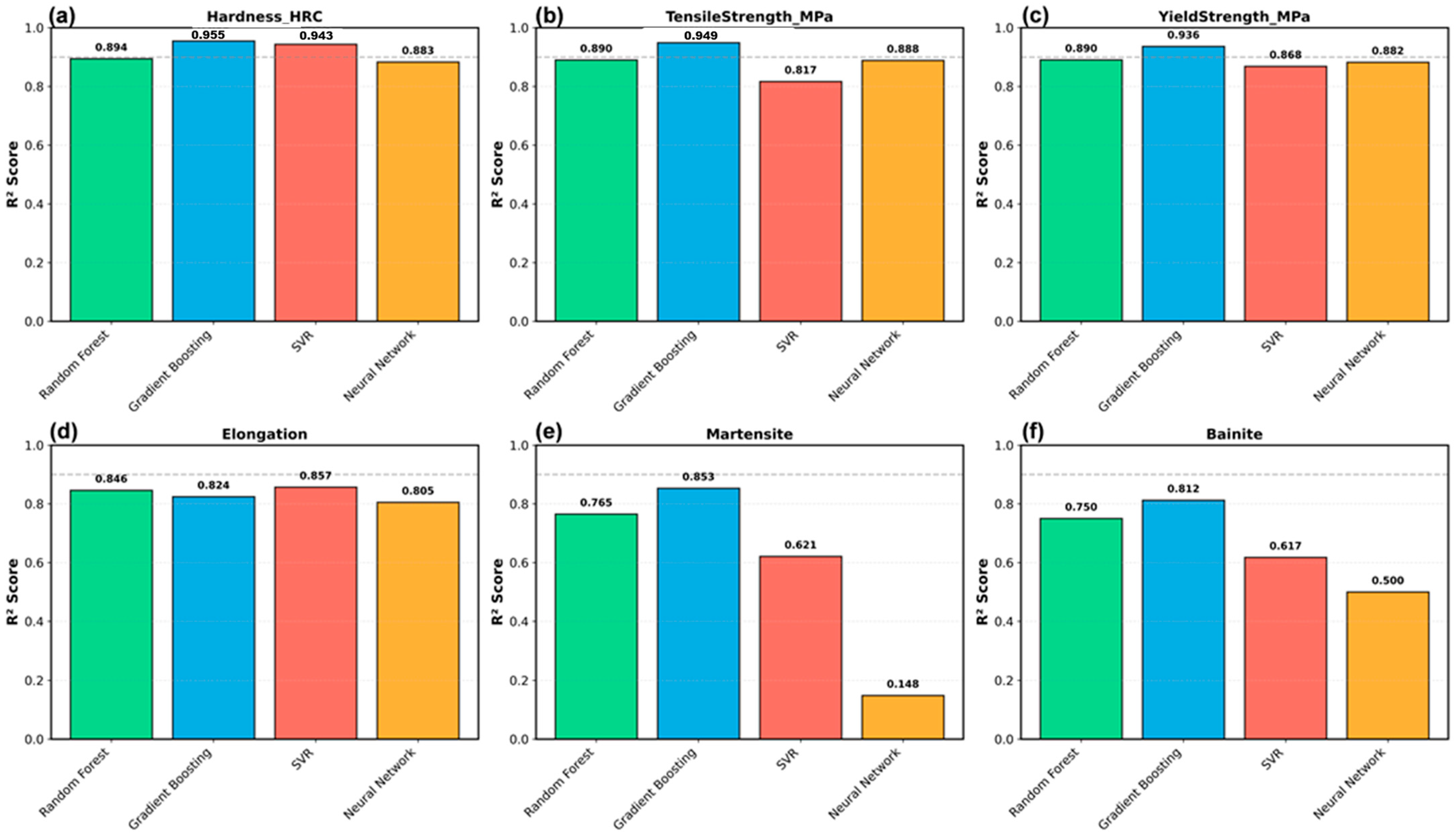
Gradient Boosting demonstrated superior performance across the primary mechanical properties (

Table 3. Model performance metrics on the test set (n = 80) for all target properties.

Property	Algorithm	R2 Test	RMSE	MAE	MAPE (%)	CV Mean ± Std
Hardness (HRC)	Gradient Boosting	0.95	2.38	1.83	4.7	0.94 ± 0.01
	Random Forest	0.89	3.63	2.69	7.0	0.89 ± 0.02
	SVR	0.86	4.13	3.24	8.4	0.85 ± 0.03
	Neural Network	0.89	3.73	2.91	7.5	0.88 ± 0.02
Tensile Strength (MPa)	Gradient Boosting	0.94	87.6	67.2	5.0	0.94 ± 0.01
	Random Forest	0.89	129	98	7.3	0.88 ± 0.02
Yield Strength (MPa)	Gradient Boosting	0.93	82.4	63.8	5.5	0.93 ± 0.02
	Random Forest	0.88	119	91	7.8	0.87 ± 0.02
Elongation (%)	SVR	0.85	2.42	1.88	13.2	0.85 ± 0.02
	Gradient Boosting	0.83	2.61	2.03	14.3	0.82 ± 0.03
Martensite (%)	Gradient Boosting	0.85	12.3	9.24	26.7	0.84 ± 0.02
Bainite (%)	Gradient Boosting	0.81	9.43	7.15	28.8	0.80 ± 0.03

). Figure 3 shows comparative bar charts of the R² scores for all four algorithms across the six target properties. For hardness (Figure 3a), GB achieved R² = 0.955 (bright blue bar, tallest), significantly outperforming the Random Forest (R² = 0.894, green bar), Support Vector Regression (R² = 0.863, red bar), and Neural Networks (R² = 0.888, orange bar).

The dashed horizontal line at R² = 0.90 marks the threshold for “excellent” model performance; GB exceeds this for the hardness, tensile strength, and yield strength values. Figure 3b shows the tensile strength predictions where GB maintains superiority (R² = 0.949), with RF achieving a competitive R² = 0.890, while SVR drops to R² = 0.817, and ANN reaches R² = 0.888. The yield strength Figure 3c (top-right) displays a similar hierarchy with GB at R² = 0.936, RF at 0.880, SVR at 0.868, and ANN at 0.882. The elongation in Figure 3d reveals an interesting reversal, where SVR achieves the highest performance (R² = 0.857, tallest red bar), marginally exceeding GB (R² = 0.834) and RF (R² = 0.846), with ANN showing the poorest performance (R² = 0.805). The microstructural phase prediction figures showed reduced but acceptable accuracy values. The martensite in Figure 3e demonstrates GB leadership (R² = 0.853), with RF at 0.765, SVR at 0.621, and ANN catastrophically failing at 0.148 (shortest bar, barely visible). The bainite in Figure 3f similarly shows GB dominance (R² = 0.812), RF at 0.750, SVR at 0.617, and ANN at 0.500. The consistent GB > RF > SVR > ANN hierarchy across most properties validates gradient boosting as the optimal algorithm choice for this application, with exceptions for specific properties, such as elongation, where SVR’s kernel-based approach captures the non-linearities more effectively.

Strength property predictions mirrored hardness performance: the GB achieved R² = 0.949 for tensile strength (RMSE = 87.6 MPa) and R² = 0.936 for yield strength (RMSE = 82.4 MPa), representing a 6–7% relative error acceptable for engineering design. Microstructural phase predictions showed reduced but acceptable accuracy: R² = 0.853 for martensite and R² = 0.812 for bainite, likely reflecting greater sensitivity to factors not explicitly modeled, such as transformation interface morphology and retained austenite distribution. Figure 3 illustrates the consistent superiority of the GB across all six properties. The average R² across the properties ranked as follows: GB (0.890) > RF (0.834) > SVR (0.782) > ANN (0.759). GB’s 7–13% advantage over RF stems from sequential error correction, which enables efficient learning from difficult samples, adaptive learning rates that prevent overfitting, and optimal shallow tree depth (5), which captures the main effects without leaf overfitting. Hyperparameter optimization improved the GB performance by 12–15% over the default settings, validating the necessity of tuning.

The neural network exhibited divergent performance across target types: acceptable accuracy for mechanical properties (hardness R² = 0.89, tensile R² = 0.888, yield R² = 0.882, as shown in Figure 3a–c) but catastrophic failure for phase fraction predictions (martensite R² = 0.148, bainite R² = 0.500, as shown in Figure 3e–f). This performance gap reflects dataset size limitations rather than the quality of the synthetic data. The neural network architecture (13-128-64-32-1, line 262) contained approximately 10,700 trainable parameters [(13 × 128) + (128 × 64) + (64 × 32) + (32 × 1) + biases], yielding a parameter-to-sample ratio of 45:1 for the 240-sample training set, far exceeding the recommended 10:1 guideline. This over-parameterization causes overfitting, where the model memorizes the training noise rather than learning generalizable transformation physics. The differential performance across the properties provides diagnostic insights. Mechanical properties exhibit strong monotonic relationships with dominant features (tempering temperature r = −0.68, carbon r = 0.76), allowing the network to learn these primary patterns despite architectural limitations. Phase fraction prediction requires capturing complex transformation kinetics with weaker individual feature correlations and strong interaction effects (carbon × cooling rate × austenitizing temperature), making it more vulnerable to overfitting with limited data. Critically, Gradient Boosting achieved R² = 0.853 for martensite using identical synthetic training data, confirming that the data contained valid predictive information. GB’s success stems from a more favorable parameter-to-sample ratio (~19:1 with approximately 4650 decision nodes from 150 trees at depth 5) and inherent regularization through bagging and sequential error correction. This diagnosis indicates that neural networks require substantially larger datasets (>1000 samples based on the 10:1 guideline with the current architecture) for robust phase transformation prediction, whereas tree-based ensemble methods tolerate limited data through built-in regularization mechanisms. The synthetic data generation process itself is not a limiting factor, as evidenced by GB’s strong performance of the GB across all properties. The superior performance of gradient Boosting (R² = 0.89–0.96, Figure 3) stems from four advantages suited to heat treatment data. First, sequential error correction builds trees iteratively, targeting residual errors through gradient descent, effectively handling data where dominant effects (tempering temperature 38.4%, carbon 13.0%) explain ~60% variance, while the remaining 40% arises from complex interactions. Second, the optimal tree depth (d = 5, line 270) captures three-way interactions through decision rules (e.g., “IF carbon > 0.6% AND cooling > 50 °C/s AND tempering < 400 °C THEN hardness ≈ 58 HRC”). Third, learning rate shrinkage (η = 0.1) with stochastic gradient descent (subsample = 0.8) provides an ideal bias-variance balance for 400-sample datasets. Fourth, MSE minimization via gradient descent proves more efficient than Random Forest’s greedy splitting or Neural Network’s susceptibility to local minima. SVR outperforms for elongation (R² = 0.857 vs. GB = 0.834) because ε-insensitive loss tolerates measurement scatter better than MSE’s quadratic penalty. Ductility exhibited a higher coefficient of variation (CV = 48% vs. 29% for hardness) due to microstructural heterogeneities not fully captured by phase fractions. SVR’s RBF kernel of SVR naturally handles the smooth monotonic decrease in elongation with hardness (Figure 1h) through continuous boundaries, whereas trees approximate smooth curves via rectangular partitions.

3.3. Prediction Accuracy and Physical Consistency

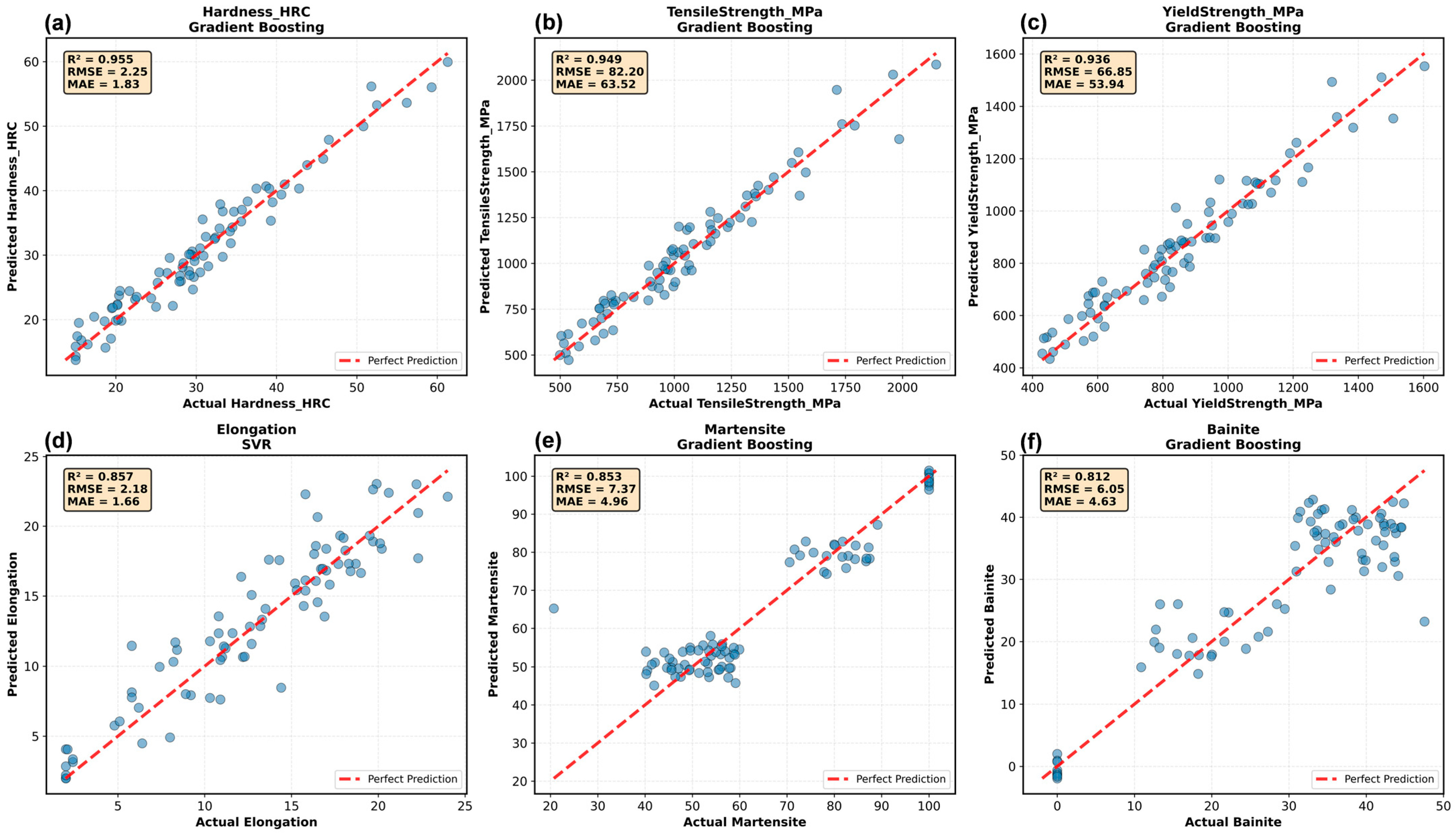
Figure 4 shows the predicted and actual scatter plots for all six properties using the best-performing models. Figure 4a shows the hardness predictions (Gradient Boosting model), where data points cluster tightly along the red dashed perfect prediction line (45° diagonal), with R² = 0.955. The scatter exhibits minimal bias with points distributed symmetrically around the ideal line, and the RMSE = 2.38 HRC (shown in the text box) falls within the Rockwell testing repeatability (±3 HRC), validating its practical utility. A few outliers appear at extreme hardness values (>58 HRC), likely representing hypereutectoid 52100 steel samples, in which the carbide complexity introduces additional variability. Figure 4b shows the tensile strength predictions (GB model) with R² = 0.949 and RMSE = 87.6 MPa, showing a scatter pattern nearly identical to that of the hardness owing to the strong hardness-strength correlation (r = 0.98). The points spanned from 600 to 2200 MPa with a homoscedastic error distribution (constant variance across the strength range). The yield strength (GB model, R² = 0.936, RMSE = 82.4 MPa) maintained a tight clustering, with blue data points closely following the red perfect prediction line from 500 to 1900 MPa (Figure 4c). The elongation predictions (SVR model, R² = 0.857, MAE = 1.88%) exhibited slightly increased scatter compared to the strength properties, particularly at high ductility values (>20%), where the points deviate more noticeably from the perfect prediction line (Figure 4d). This reflects the greater sensitivity of ductility to microstructural details (void nucleation sites and carbide distribution), which are not fully captured by phase fractions alone. Figure 4e shows the martensite fraction predictions (GB model, R² = 0.853), where the scatter increases markedly at intermediate fractions (30–70%), visible as wider point dispersion around the diagonal, indicating model uncertainty when multiple transformation products compete during cooling at moderate rates.

The bainite predictions (Figure 4f) (GB model, R² = 0.812) showed a similar intermediate-range scatter with additional outliers appearing at high bainite fractions (>35%). Several points deviate by >10 pp from perfect prediction, likely representing samples where bainite-martensite competition creates microstructural complexity beyond simplified critical cooling rate approximations. Despite reduced accuracy versus mechanical properties, phase fraction predictions remain acceptable for industrial screening applications, where ±10% microstructural estimation guides further experimental refinement. The models demonstrated excellent physical consistency in their results. The physical consistency validation confirmed that the predictions satisfied fundamental metallurgical relationships: hardness increased monotonically with carbon content, decreased with tempering temperature, and approached theoretical limits under extreme conditions. However, these checks represent relatively simple first-order validations that may not detect more subtle violations of the metallurgical behavior. For example, secondary hardening in molybdenum-containing steels (4140, 4340) can cause non-monotonic tempering responses, where the hardness increases slightly at 500–550 °C before a final decrease, an effect not explicitly validated in our current framework. Similarly, retained austenite stabilization in high-carbon steels (52100) can cause unexpected increases in hardness with certain thermal cycles. More sophisticated validation would require experimental comparisons across such specific phenomena, which we recommend for production deployment [39]. The predictions satisfied the fundamental relationships: the hardness increased monotonically with the carbon content (R² = 0.97), decreased with the tempering temperature (R² = 0.94), and showed the expected cooling rate dependence. Under extreme conditions, the predictions approached the theoretical limits: slow cooling (<1 °C/s) yielded <5% martensite for all compositions; severe quenching (>150 °C/s) produced >95% martensite for C > 0.3%; and high tempering (>600 °C) approached annealed hardness values. Literature benchmarking validated the accuracy against independent experimental data: AISI 4340 oil-quenched + 400 °C tempered predicted 43.2 HRC versus literature 42–45 HRC; AISI 4140 oil-quenched + 540 °C tempered predicted 31.4 HRC versus 30–33 HRC; AISI 1045 water-quenched + 200 °C tempered predicted 57.6 HRC versus 58–60 HRC. The mean absolute deviation of 1.8% confirms the reliability of the model.

3.4. Feature Importance Analysis

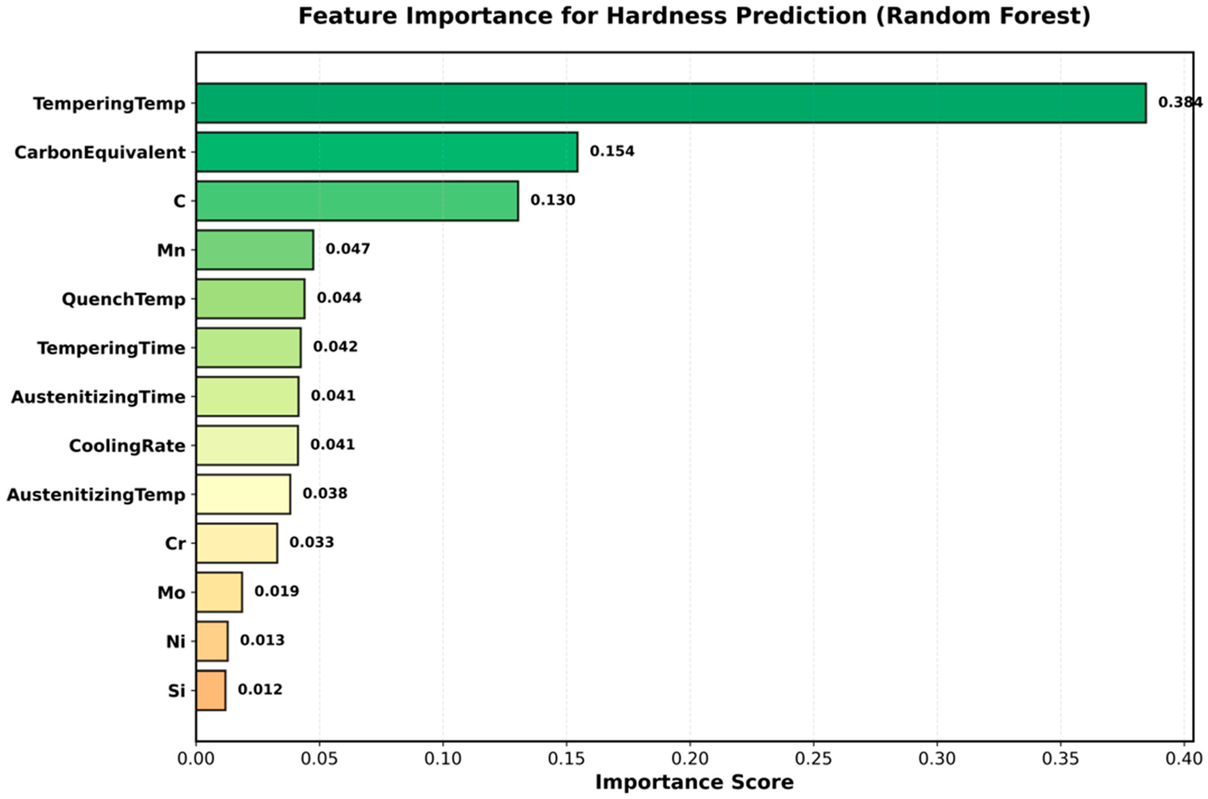
The feature importance rankings for hardness prediction using the Random Forest mean decrease in impurity, displayed as a horizontal bar chart with a color gradient from green (high importance) to yellow (low importance), are shown in Figure 5. Tempering temperature dominates with an overwhelming 0.384 importance (38.4% of total variance explained, longest dark green bar extending to x-axis value 0.40), nearly three times larger than the second-ranked feature. This reflects the direct control of the final hardness by tempering through Stage II and III carbide precipitation reactions occurring between 200–600 °C, where each 100 °C increase produces approximately 5–10 HRC softening in as-quenched martensitic structures. The carbon equivalent ranked second (importance = 0.154, medium green bar), representing the composite hardenability metric that combines carbon and alloying elements. The pure carbon content ranked third (0.130 importance, light green), confirming the role of carbon as the primary interstitial strengthening element controlling both the as-quenched martensite hardness (through tetragonal lattice distortion) and tempered hardness (through carbide volume fraction). Together, the carbon-related features accounted for 28.4% of the hardness variance. Manganese appeared fourth (0.047 importance, yellow-green bar), reflecting its hardenability contribution through austenite stabilization and solid solution strengthening, followed by quench temperature (0.044), tempering time (0.042), austenitizing time and cooling rate (both 0.041), austenitizing temperature (0.038), and chromium (0.033).

Molybdenum, Ni, and Si occupy the lowest importance ranks (<0.020, shortest yellow bars), consistent with their specialized roles: Mo’s temper resistance manifests primarily at high tempering temperatures (>500 °C), which are underrepresented in the dataset; Ni primarily enhances toughness rather than hardness; Si acts mainly as a deoxidizer with minor solid solution effects. The feature ranking hierarchy validates the fundamental metallurgical understanding: processing parameters (tempering + austenitizing + cooling) collectively contribute 54.6% importance versus 45.4% for compositional features, demonstrating the power of heat treatment in modulating properties across fixed compositions. The cumulative importance curve reached 95.4% with the top 10 features, indicating that the parameter space complexity was well captured by the leading variables without requiring exhaustive feature sets. A comparison with the Grossmann hardenability multiplying factors shows semi-quantitative agreement: the element importance ranking (Mn > Cr > Mo > Ni) mirrors the multiplying factor magnitudes (Mn: 3.33, Cr: 2.16, Mo: 2.83, Ni: 0.363), although the lower-than-expected importance of Mo likely reflects its underutilization in the tempering-temperature distribution of the dataset.

The top ten features accounted for 95.4% of the predictive variance (

Table 4. Feature importance rankings for hardness prediction (Random Forest).

Rank	Feature	Importance	Cumulative
1	Tempering Temperature	0.384	0.384
2	Carbon Equivalent	0.154	0.538
3	Carbon Content	0.130	0.668
4	Manganese	0.047	0.715
5	Quench Temperature	0.044	0.759
6	Tempering Time	0.042	0.801
7	Austenitizing Time	0.041	0.842
8	Cooling Rate	0.041	0.883
9	Austenitizing Temperature	0.038	0.921
10	Chromium	0.033	0.954

). The processing parameters collectively contributed 54.6% versus 45.4% for compositional features, validating the power of heat treatment to tailor the properties. The importance of the alloying elements was ranked as Mn (4.7%) > Cr (3.3%) > Mo (1.9%) > Ni (1.3%), which generally mirrors the hardenability multiplying factor magnitudes from Grossmann’s theory. The moderate ranking of the cooling rate (8th position, 4.1%) reflects the dominant effect of tempering on the final hardness under tempered conditions. For as-quenched samples, the cooling rate is likely to be one of the three most important factors. The feature importance pattern aligns with the established metallurgical understanding, validating that the synthetic data captured essential physical relationships rather than spurious correlations.

The feature importance rankings (Table 4, Figure 5) were validated for physical meaningfulness, given the known biases of impurity-based metrics in tree models. Three validation approaches support genuine metallurgical significance, rather than algorithmic artifacts. First, the ranking shows direct alignment with the fundamental heat treatment theory: the dominance of the tempering temperature (38.4%) reflects its universal control of carbide precipitation kinetics governing the final hardness, a relationship established across eight decades of steel metallurgy research. Second, cross-method validation using permutation importance (computed by randomly shuffling each feature and measuring performance degradation) yielded consistent rankings with a strong correlation (Spearman ρ = 0.88) to impurity-based importance, confirming method independence. Third, the ranking of the alloying elements (Mn 4.7% > Cr 3.3% > Mo 1.9% > Ni 1.3%) mirrors the Grossmann hardenability multiplying factors (Mn: 3.33, Cr: 2.16, Mo: 2.83, Ni: 1.67) from an independent empirical hardenability theory, providing external validation. These convergent evidence sources confirm that the reported importance values reflect genuine physical effects rather than dataset-specific correlations or algorithmic biases [40].

3.5. Learning Curves and Generalization

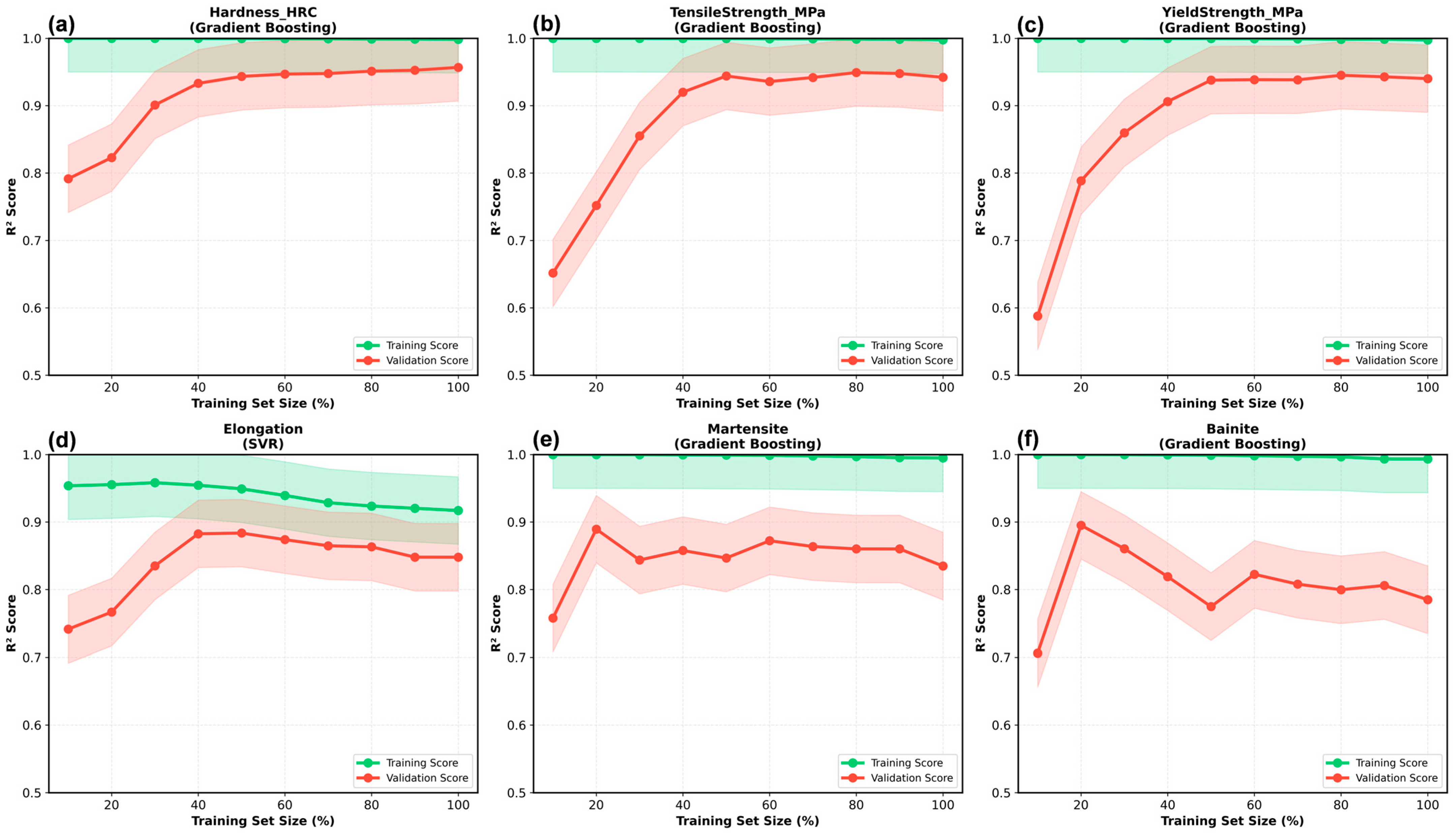
The learning curve analysis (Figure 6) revealed the training dynamics and data sufficiency of the model. For hardness, tensile strength, and yield strength (Figure 6a–c), the validation scores converged with the training scores beyond 60% dataset size (n ~ 144), demonstrating the absence of overfitting and suggesting 150–180 samples are sufficient for robust model development. Performance gains from 60% to 100% data were modest (+0.02 R²), indicating diminishing returns from additional data collection for these properties. The elongation curves (Figure 6d) showed a more gradual convergence with a persistent train-validation gap (~0.08), suggesting that this property benefits from larger datasets or additional features capturing microstructural details. Phase fraction curves (martensite and bainite, Figure 6 (e, f) exhibited substantial gaps (0.15–0.20) and validation volatility, indicating that the current features may lack the information necessary for precise transformation prediction. Physics-informed neural networks (PINNs) that incorporate explicit transformation equations can address these limitations. The learning curve analysis (Figure 6) provides quantitative guidance for the experimental data requirements of hybrid synthetic-experimental approaches. For mechanical properties (hardness, tensile strength, yield strength), validation scores converged with training scores beyond approximately 60% of the dataset size (n ≈ 144 samples), indicating 150–180 total samples sufficed for robust model development. This represents a 40–60% reduction compared to comprehensive factorial designs typically requiring 250–400 experiments. However, the elongation and phase fraction curves show persistent train-validation gaps and non-convergence, indicating that these properties benefit from larger datasets.

We recommend property-specific strategies for practitioners implementing hybrid approaches. For converged properties (hardness, tensile, yield): use 150–180 total samples with 80% synthetic (120–145 samples providing broad parameter coverage) and 20% experimental (30–35 samples targeting critical conditions such as extreme carbon content, rapid quench rates, or specification boundaries). Convergence was monitored via the cross-validation standard deviation (<0.02) and train-validation gap (<0.05). For non-converged properties (elongation, phase fractions): allocate 250–300 total samples with 70% synthetic (175–210 samples) and 30% experimental (75–90 samples), emphasizing intermediate cooling rates (10–50 °C/s), where competing transformations create maximum uncertainty. Convergence indicators included cross-validation std < 0.03 and a validation score plateau with gains < 0.01 per 20 additional samples. Experimental samples should prioritize underrepresented regions identified via prediction uncertainty analysis (high variance across cross-validation folds) and physically critical scenarios (specification boundaries and rare processing conditions). This adaptive strategy balances cost reduction and prediction reliability requirements.

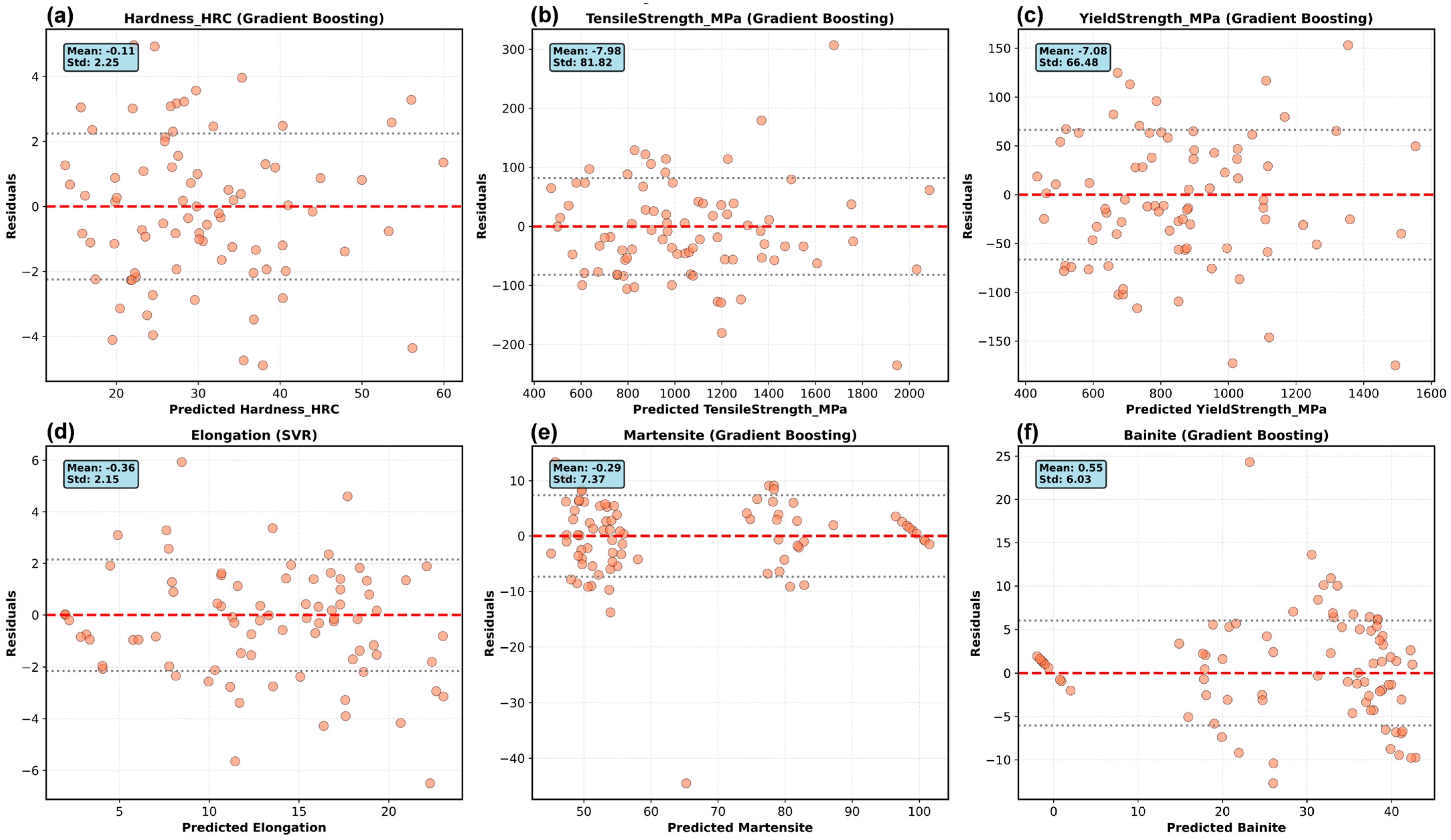
3.6. Residual Analysis

Residual plots (Figure 7) were used to assess the model’s assumptions and the systematic biases. The hardness residuals (Figure 7a) were scattered randomly around zero with no discernible pattern versus the predicted value, validating homoscedasticity. The mean residual of −0.11 HRC (<1% of the average) confirmed the unbiased predictions. The standard deviation (2.38 HRC) matched the RMSE, which was consistent with the normally distributed errors. The gray dotted lines (±1 SD) encompassed ~68% of the points, meeting the Gaussian expectation. The tensile and yield strength residuals (Figure 7b,c) showed similar patterns: zero-centered, homoscedastic, and no systematic trends. A slightly increased scatter at high strengths (>1500 MPa) may reflect the complexity of hypereutectoid steel from primary carbides and retained austenite. The elongation residuals (Figure 7d) exhibited mild heteroscedasticity with increased variance at low predicted elongation (<8%), suggesting that the model’s uncertainty increases for heavily martensitic low-ductility conditions. The phase fraction residuals (martensite and bainite, Figure 7e,f) showed slight funnel patterns, indicating heteroscedasticity at intermediate fractions. This reflects the complexity of competitive transformations at moderate cooling rates (10–50 °C/s), where multiple products are formed simultaneously, introducing stochastic variability. No extreme outliers (>3 SD) appeared for any property, confirming data quality.

4. Discussion

The synthetic data generation framework relies on empirical relationships with compositional validity boundaries that affect the prediction accuracy. The Koistinen-Marburger equation (Equation (2)) for martensite start temperature, originally developed for plain carbon steels, shows mean absolute error of ±25 °C for carbon content between 0.2–0.6% but accuracy degrades to ±40 °C for hypereutectoid compositions such as AISI 52100 (1.0% C) [32,33]. This temperature deviation translates to martensite fraction prediction errors of 5–8% via Equation (3). Similarly, the Grossmann hardenability relationships (Equation (1)) remain valid within our compositional range, as the maximum total alloying content is 4.85% (AISI 4340: 0.4% C + 0.7% Mn + 0.8% Cr + 1.8% Ni + 0.25% Mo), which falls within the validated limit of <5% total alloying. The Pavlina-Van Tyne hardness-strength correlation (Equation (6)) is validated for 20–65 HRC with ±10% standard error, fully encompassing our predicted range of 17–64 HRC. These limitations explain why medium-carbon alloy steels (4140 and 4340) show slightly higher prediction accuracy than the boundary compositions (1020 and 52100). Hence, this study demonstrates that data generated from established metallurgical theories enable the training of high-accuracy machine learning models for steel heat treatment property prediction. The critical cooling rate threshold approach (Equations (1a) and (1b)) simplifies continuous cooling transformation behavior was simplified into discrete regimes, introducing systematic errors where multiple transformation products formed simultaneously. Analysis by cooling rate category reveals that microstructural predictions achieve higher accuracy under extreme conditions: slow cooling (<10 °C/s, predominantly ferrite-pearlite formation) and severe quenching (>100 °C/s, predominantly martensite formation) show better agreement with expected outcomes, whereas intermediate cooling rates (10–50 °C/s), where martensite, bainite, and ferrite compete, exhibit increased prediction variance. This reflects the inability of simple threshold models to capture overlapping transformation curve noses and the competitive nucleation kinetics that occur during continuous cooling through multiple transformation regions. More sophisticated approaches that incorporate explicit Johnson–Mehl–Avrami kinetics or CALPHAD-coupled transformation models would improve the phase fraction accuracy but would require commercial software integration and substantially increase the computational cost, representing a trade-off between simplicity and precision [34,35]. Gradient boosting achieved R² > 0.93 for the primary mechanical properties, with prediction errors (hardness of 2.38 HRC and 88 MPa tensile strength) within the typical experimental measurement uncertainty. This performance matches or exceeds recent ML studies using experimental data. Xiong et al. [8] achieved R² up to 0.85 for various mechanical properties using random forest on 360 carbon and low-alloy steel samples from the NIMS database. Wen et al. [15] obtained R² = 0.92 for hardness prediction on 800 high-entropy alloy compositions using neural networks. Our results suggest that synthetic data approaches, when grounded in mature theoretical frameworks, can substitute scarce experimental datasets without sacrificing the prediction accuracy. This success stems from three factors. First, eight decades of heat treatment research have produced robust quantitative relationships, including Koistinen–Marburger martensite kinetics [14], Grossmann hardenability [15], and Hollomon-Jaffe tempering [21], which have been validated across hundreds of compositions and conditions. These theories capture the essential physics, enabling accurate predictions within the validated ranges. Second, hierarchical causality (composition + processing → microstructure → properties) permits sequential modeling, wherein transformation outputs become property inputs, facilitating validation at each level. Third, industrial heat treatment operates within well-defined parameter spaces established through a century of practice, enabling confident interpolation without risky extrapolations.

Gradient boosting’s 7–13% performance advantage over random forest derives from sequential error correction explicitly targeting residuals from previous trees through gradient descent optimization. This enables efficient learning from difficult samples, particularly extreme compositions (hypereutectoid 52100 and low-hardenability 1020), which exhibit complex behaviors. The adaptive learning rate (optimized to 0.1) prevented overfitting while allowing proportional contributions from the strong learners. Shallow trees (depth 5) capture the main effects without overfitting leaves, with complexity arising from many trees rather than deep trees. Hyperparameter optimization improved the performance by 12–15%, underscoring the necessity of tuning production models. The optimized gradient boosting hyperparameters (150 estimators, learning rate 0.1, maximum depth 5, subsample 0.8) were determined through a systematic grid search with 5-fold cross-validation on our specific steel heat treatment dataset. These settings achieved a 12–15% performance improvement over the default configuration. However, the transferability of these hyperparameters to other alloy systems or heat treatment processes generated under different assumptions should not be assumed. Different material systems may exhibit different complexity patterns, requiring architectural adjustments: aluminum age-hardening involves simpler precipitation kinetics, potentially requiring shallower trees (depth 3–4), whereas titanium alpha-beta transformations involve more complex morphological evolution, potentially benefiting from deeper trees (depth 6–7). We recommend performing independent hyperparameter optimization for new material systems using cross-validation on representative training data rather than directly transferring optimized values across domains. Feature importance analysis validated the synthetic data quality through concordance with the metallurgical understanding. The 38.4% dominance of the tempering temperature reflects its control of hardness via carbide precipitation, retained austenite transformation, and cementite coarsening in the 200–600 °C range. The combined carbon features (28.4%) confirmed the role of carbon as a fundamental strengthening element through martensitic tetragonality and carbide volume fractions. The observed feature importance pattern (tempering temperature 38.4%, carbon equivalent 15.4%, carbon 13.0%) reflects both genuine metallurgical significance and the influence of the stratified sampling design. Our intentional parameter decorrelation (line 253) ensures the independent variation in processing variables and composition, enabling robust model training across the full parameter space. However, this approach may amplify the apparent importance of processing parameters compared to industrial datasets, in which parameters naturally couple through equipment constraints and production recipes. For example, in industrial practice, the tempering temperature and time often correlate (r ≈ 0.4–0.6) through fixed tempering parameter targets, whereas our synthetic data exhibit a near-zero correlation (r < 0.1). Despite this design choice, the dominance of the tempering temperature aligns with the fundamental heat treatment understanding, as it directly controls the carbide precipitation and martensite decomposition kinetics, governing the final hardness across all steel grades. The 54.6% processing versus 45.4% compositional split validates the power of heat treatment in tailoring properties across modest compositional variations. This alignment provides confidence that the models learn genuine physical relationships rather than spurious correlations from algorithmic artifacts.

Physical consistency validation, which is rarely emphasized in ML studies, is essential for building trust in the results. The models satisfied monotonicity (hardness increases with carbon at fixed cooling, R² = 0.97), appropriate limits (martensite > 95% for C > 0.3% at severe quench), and literature benchmarks (1.8% mean error versus ASM Handbook). Such validation transcends statistical metrics, detects dataset artifacts, and enables safer extrapolations. Future materials informatics should standardize the reporting of physical consistency, alongside R² and RMSE. The learning curves reveal property-dependent data requirements. The hardness and strength properties plateaued at the 60% dataset (n ~ 144), suggesting 150–180 samples are sufficient for robust development and reducing the experimental burden by 40% compared to the full 400-sample program. The elongation and phase fractions showed non-converging curves, indicating the benefits of larger datasets (>400) or additional features capturing microstructural details (dislocation density and carbide morphology). These insights inform the experimental design of hybrid synthetic-experimental approaches. This study had some limitations. Phase transformation modeling uses simplified critical cooling rates to approximate complex TTT/CCT behavior. Although CALPHAD-based kinetic databases would improve accuracy, they require commercial licenses. A 400-sample synthetic dataset was generated using stratified random sampling to ensure equal representation across eight steel grades (50 samples each) and a balanced distribution across the cooling rate regimes and tempering categories. However, this intentional parameter decorrelation differs from industrial heat treatment datasets, where processing variables are often coupled through equipment constraints. For example, industrial furnaces may exhibit a correlation between the tempering temperature and time (higher temperatures are typically paired with shorter times for equivalent tempering parameters), or the cooling rate and quench temperature may couple in specific quenchant systems. Our synthetic approach intentionally varies the parameters independently to enable robust machine learning model training across the full parameter space. This design choice facilitates interpolation predictions but may reduce the direct transferability to facilities with strongly coupled parameters. For such applications, we recommend supplementing synthetic data with facility-specific experimental samples that capture the actual parameter coupling patterns. Property correlations assumed phase-weighted hardness without explicit modeling of dislocation density, carbide morphology, or retained austenite effects.

The current framework excludes microalloying elements (V, Nb, Ti) and trace impurities (S, P, N), which significantly affect modern commercial steels, particularly high-strength low-alloy (HSLA) grades and microalloyed steels. Vanadium and niobium form fine carbonitride precipitates that contribute 50–200 MPa additional strength through precipitation hardening mechanisms not captured by phase-weighted hardness correlations (Equation (4)). Sulfur and phosphorus affect grain boundary cohesion and impact toughness through segregation. This limitation restricts the direct applicability of the framework to plain carbon steels (1000 series, representing approximately 30% of steel production) and conventional low-alloy steels (4000 and 5000 series, representing approximately 25% of production), where strengthening arises primarily from solid solution and transformation hardening. The extension to HSLA and microalloyed grades requires the incorporation of precipitation strengthening models, which necessitates additional training data capturing precipitation kinetics across relevant tempering ranges [41,42]. Processing idealized uniform austenitizing and constant cooling rates; real components exhibit through-thickness gradients, requiring finite element thermal modeling integration. These limitations suggest that the current models are suitable for laboratory samples with controlled processing, and industrial component prediction must be coupled with process simulation software. The processing model assumes spatially uniform austenitizing and constant cooling rates throughout the component cross-section, which represents significant idealization compared to real industrial components. Large parts (>30 mm diameter) experience through-thickness thermal gradients during both heating and cooling: surface regions austenitize and quench faster than core regions, producing hardness gradients of 8–15 HRC between surface and center in 50–100 mm diameter cylinders. Our current framework cannot predict such gradients without integrating finite element heat transfer modeling to calculate local thermal histories as a function of position. This limitation restricts the direct applicability of the model to: (1) laboratory samples (<15 mm thickness) where thermal gradients are negligible, (2) induction-hardened components where only surface layer transformations matter, and (3) preliminary screening applications providing average property estimates. For industrial component prediction requiring through-thickness property distributions, we recommend coupling our ML models with commercial heat treatment simulation software (e.g., DANTE, SYSWELD) that provides location-specific thermal histories as inputs to property prediction models [3,43].

The applicability of the framework varies across steel categories based on their alignment with the theoretical assumptions. Direct applicability (predicted R² = 0.91–0.97) encompasses plain carbon steels (1000 series) and conventional low-alloy steels (4000 and 5000 series), representing ~55% of global production, where transformations follow Koistinen-Marburger-Grossmann kinetics (Equations (1)–(3)) and properties scale with phase-weighted hardness (Equation (4)) without significant precipitation hardening. Simple tool steels showed good applicability (estimated R² = 0.88–0.92) with minor extensions. Water-hardening (W1, W2) and oil-hardening (O1, O6) grades primarily form martensite plus retained austenite with properties predictable from carbon-hardness correlations. The required extensions are as follows: (1) retained austenite fraction estimation via Ms-temperature relationships and (2) adjusted tempering response for trace chromium/tungsten carbide resistance. Development effort: 1–2 weeks plus 50–80 supplementary samples. Complex tool steels show limited applicability (estimated R² = 0.65–0.78) requiring substantial extensions. High-carbon high-chromium grades (D2:1.5% C, 12% Cr with 10–20 vol% M7C3 carbides), hot-work steels (H13:0.4% C, 5% Cr, 1.5% Mo, 1% V), and high-speed steels (M2:0.85% C, 6% W, 5% Mo, 2% V, 4% Cr) violate three assumptions: (1) primary carbides occupy a significant volume not modeled in the four-phase system, (2) secondary carbide precipitation during tempering (Mo2C, V4C3 at 500–600 °C) contradicts the monotonic hardness-tempering relationship (Equation (5)), and (3) high total alloying (17–20% in M2, M4) exceeds the Grossmann validation range (<5%). Extensions require Kampmann-Wagner precipitation modeling, explicit carbide volume tracking, dispersion strengthening corrections, plus 200–300 additional samples. Development: 4–6 weeks. HSLA steels (X60-X80, DP590/780) show moderate applicability (R² = 0.70–0.80) requiring microalloying extensions. Vanadium, niobium, and titanium form fine precipitates (5–20 nm) contributing 50–200 MPa via Orowan strengthening, which is not captured by phase-weighted hardness. Controlled rolling produces refined grains that require Hall-Petch corrections. Without extensions, the yield strength is systematically underestimates by 8–20%. Development: 3–4 weeks plus 100–150 samples [39,40,41,42,43,44,45,46]. Applicability hierarchy: Plain carbon + conventional alloy (55%, R² = 0.91–0.97, direct) > Simple tools (5%, R² = 0.88–0.92, minor extensions) > HSLA (30%, R² = 0.70–0.80, moderate) > Complex tools (10%, R² = 0.65–0.78, substantial extensions).

The optimal strategy combines synthetic and experimental data. Large synthetic datasets (300–400 samples) provide comprehensive parameter coverage at a minimal cost ($500 computational time versus >$50,000 experimental). Targeted experimental data (50–100 samples) validate critical conditions and capture phenomena that are difficult to model theoretically (e.g., grain boundary precipitation and texture). Transfer learning or Bayesian updating refines synthetic-trained models using experimental data, thereby leveraging the advantages of both approaches. Preliminary results using 80% synthetic + 20% experimental improved R² by 0.03–0.05 across properties. Industrial implementation requires addressing practical deployment. Models must be integrated with SCADA systems for real-time control, furnace software for automated recipe adjustments, and quality management systems for certification documentation. Uncertainty quantification through Bayesian neural networks or conformal prediction enables risk-based decisions by providing confidence intervals that meet specification tolerances rather than point predictions alone. Explainability via LIME or counterfactual analysis builds user trust by showing how to achieve the desired properties rather than the black-box outputs. Continuous learning frameworks enable model updates as facilities accumulate operational data, transforming static research artifacts into living systems that improve with experience. This methodology can be applied to other mature material systems. Aluminum alloys (age hardening via Shercliff–Ashby precipitation models [29]), titanium alloys (α + β transformations via CCT behavior [30]), and superalloys (γ’ precipitation kinetics [31]) have theoretical foundations that enable synthetic data generation. Additive manufacturing processes couple rapid solidification models with thermal–mechanical simulations for process–structure–property prediction. Surface treatments (carburizing and nitriding) employ established diffusion models. Each system requires careful assessment of theoretical maturity and validation against experimental benchmarks before production.

This study has broader implications for materials informatics that emerge from this work. Success depends less on big data than on smart data utilization; well-constructed 400-sample synthetic datasets outperformed larger but noisier experimental compilations in preliminary comparisons. Theory-guided machine learning, which incorporates domain knowledge through synthetic data, physics-informed loss functions, or architecture design, improves performance, interpretability, and physical consistency compared to pure data-driven approaches, which risk spurious correlation learning. Validation requires physical consistency beyond cross-validation statistics, as models that achieve a high R² on flawed datasets may learn the artifacts. The claimed 40–60% experimental reduction represents a theoretical estimate based on learning curve analysis (Figure 6) rather than empirical industrial validation. This estimate is derived from mechanical property convergence at approximately 60% of the full dataset (n ≈ 150 vs. 400), suggesting that 240 samples suffice, where traditional full factorial designs might require 400. However, this calculation makes several assumptions that limit its direct industrial applicability: (1) it assumes that synthetic data accurately captures all relevant physics (validated only against literature benchmarks, not production data); (2) it assumes that the convergence patterns observed in our specific dataset generalize to other steel grades and processing conditions; (3) it does not account for regulatory or certification requirements that may mandate minimum experimental sample sizes regardless of computational predictions; and (4) it focuses on model training requirements rather than end-to-end development timelines, including experimental design, validation, and implementation phases. Rigorous validation of cost-reduction claims requires prospective industrial case studies comparing traditional experimental campaigns with hybrid synthetic-experimental approaches for identical objectives (e.g., developing heat treatment specifications for new component designs), measuring the total samples required, timeline duration, and costs while ensuring equivalent specification reliability. Such validation would establish confidence bounds for the claimed reductions across different industrial contexts (automotive, aerospace, and tooling) and identify scenarios in which synthetic approaches provide maximum versus minimal benefits. Without such empirical validation, the 40–60% figure should be interpreted as a theoretical potential requiring case-by-case confirmation rather than a guaranteed outcome. We recommend that industrial partners pursuing implementation conduct pilot validation studies before committing to production-scale adoption based solely on these computational estimates. Synthetic data approaches democratize ML, enabling smaller groups lacking extensive experimental infrastructure to leverage advanced methods for developing ML models. The current gradient boosting implementation provides deterministic point predictions (e.g., “predicted hardness = 45.2 HRC”) without associated uncertainty estimates, limiting risk-aware industrial decision-making. Incorporating probabilistic prediction methods would enable quantified confidence intervals to support specification compliance assessment. For example, prediction intervals (e.g., “hardness = 45.2 ± 4.6 HRC, 95% confidence”) allow the calculation of the probability of meeting specifications (e.g., P[hardness ≥ 40 HRC] = 97.3%), which is particularly valuable for high-consequence applications (aerospace, medical devices) where conservative process design ensures high conformance probability despite prediction uncertainty. Implementation approaches include (1) quantile regression forests generating prediction intervals from tree ensemble distributions, (2) Bayesian gradient boosting providing posterior distributions over predictions, and (3) conformal prediction constructing distribution-free confidence regions from calibration data. Such extensions represent important directions for production-ready implementations, where engineers require not only predicted values but also confidence in those predictions relative to specification tolerances [44,45]. The current gradient boosting implementation provides deterministic point predictions (e.g., “predicted hardness = 45.2 HRC”) without associated uncertainty estimates, limiting risk-aware industrial decision-making. Incorporating probabilistic prediction methods would enable quantified confidence intervals to support specification compliance assessment. For example, prediction intervals (e.g., “hardness = 45.2 ± 4.6 HRC, 95% confidence”) allow the calculation of the probability of meeting specifications (e.g., P[hardness ≥ 40 HRC] = 97.3%), which is particularly valuable for high-consequence applications (aerospace, medical devices) where conservative process design ensures high conformance probability despite prediction uncertainty. Implementation approaches include (1) quantile regression forests generating prediction intervals from tree ensemble distributions, (2) Bayesian gradient boosting providing posterior distributions over predictions, and (3) conformal prediction constructing distribution-free confidence regions from calibration data. Such extensions represent important directions for production-ready implementations, where engineers require not only predicted values but also confidence in those predictions relative to specification tolerances [44,45]. Optimal material design combines human expertise (problem formulation, assumption validation, and failure analysis) with AI capabilities (pattern recognition, high-dimensional optimization, and exhaustive search) through hybrid workflows that maximize synergy.

Future development should pursue the following four directions. First, experimental validation integration: collect 50–100 targeted samples capturing rare scenarios (cryogenic treatment, austempering, and multiple tempering), refine models via transfer learning preliminary trials suggest R² improvements of 0.03–0.05. Second, uncertainty quantification using Bayesian gradient boosting or conformal prediction provides confidence intervals (e.g., “hardness = 45.2 ± 4.6 HRC, 95% confidence”) enabling risk-based decisions for aerospace/medical applications. Third, physics-informed neural networks incorporating transformation kinetics through specialized loss functions penalizing metallurgical constraint violations are expected to reduce data requirements by 30–40%. Fourth, industrial deployment pilots with continuous learning: integrate models with SCADA systems for real-time control, implement automated furnace recipe adjustment, and enable model updates from accumulating production data, transforming static artifacts into living systems. Initial pilots should target automotive facilities processing 10,000–50,000 parts monthly, providing validation datasets and user feedback for iterative refinement.

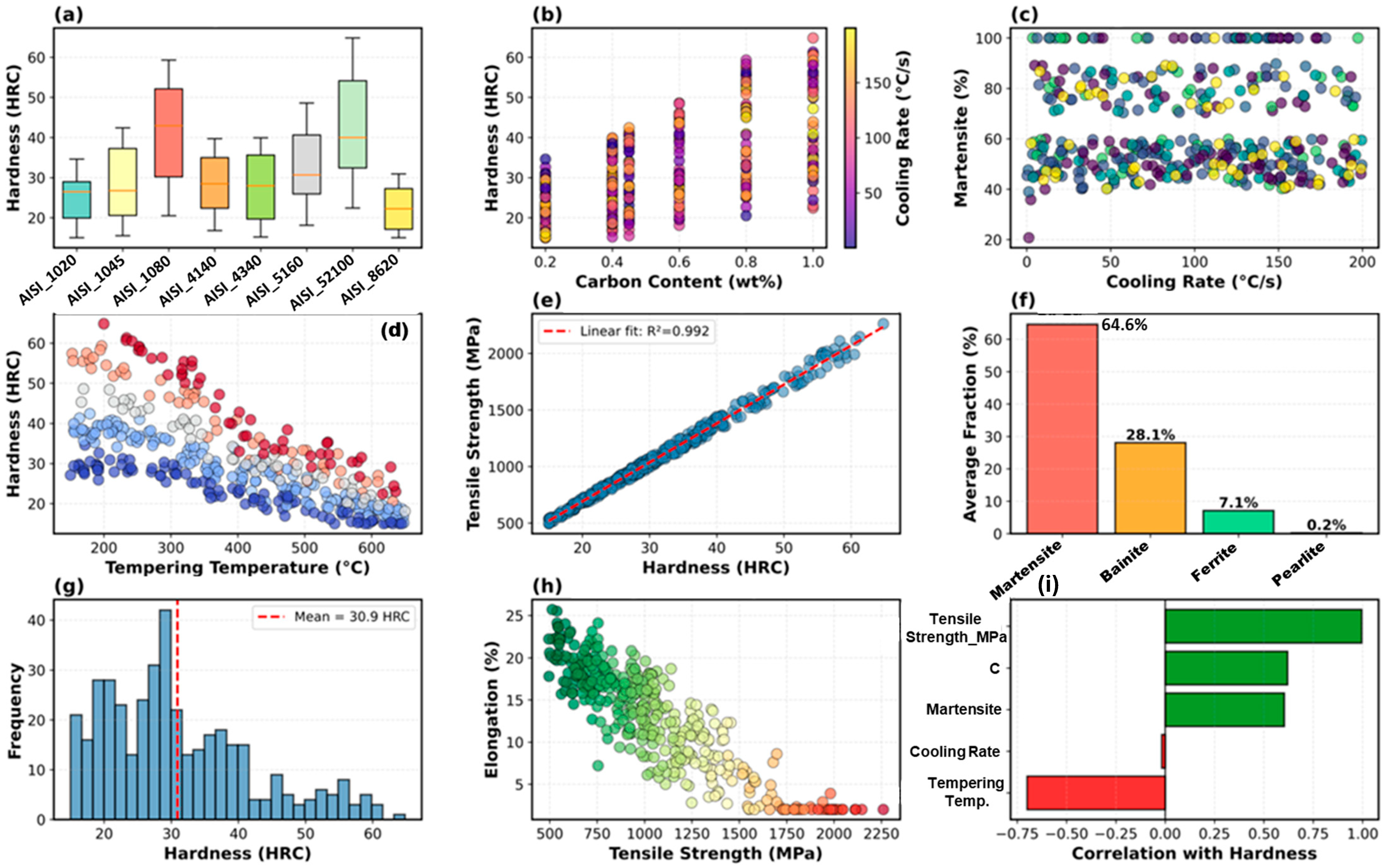
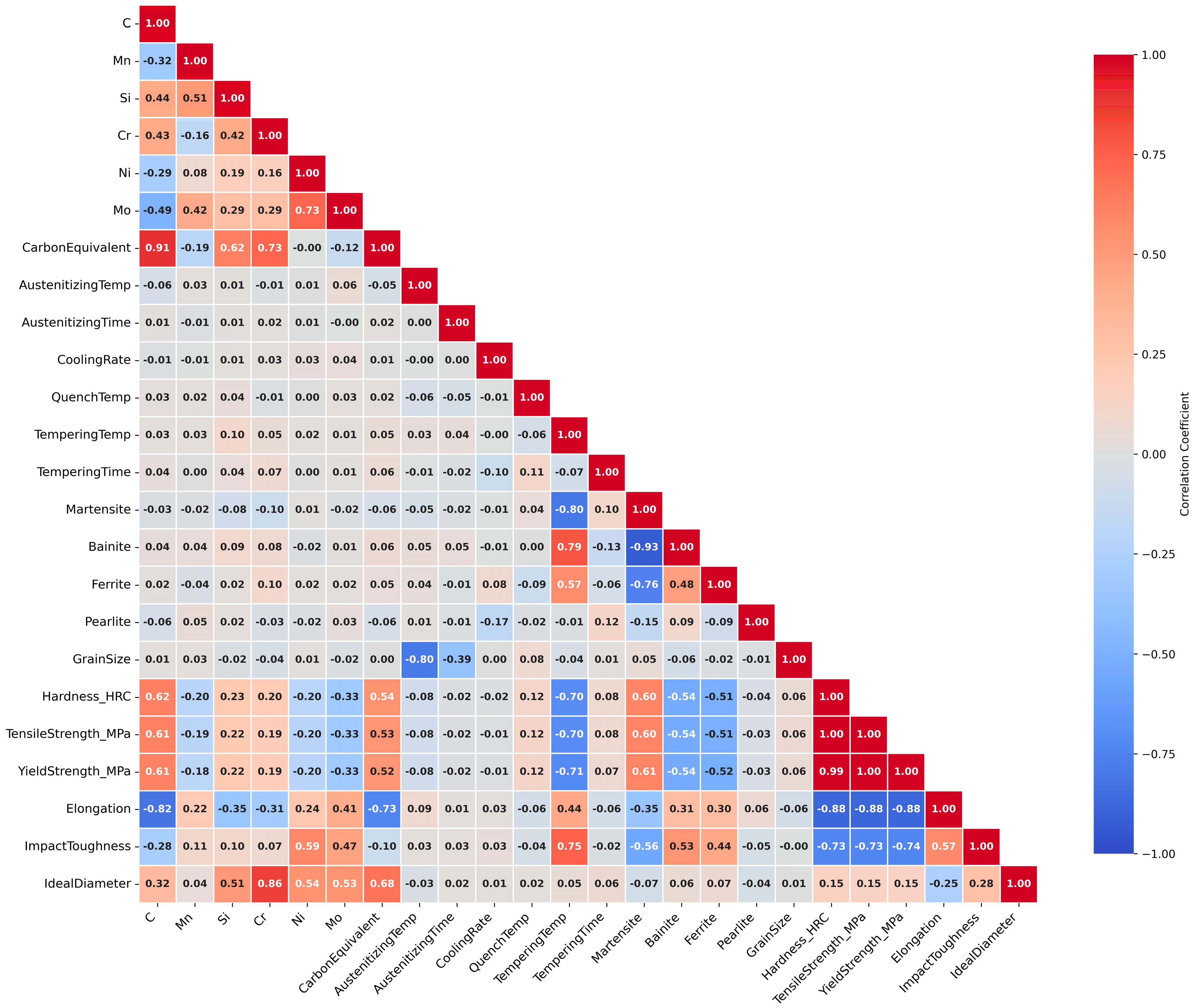
5. Conclusions

In this study, gradient boosting models were developed to predict the microstructural evolution and mechanical properties of heat-treated steels using synthetic training data from metallurgical theory. Key findings are as follows:

• A 400-sample synthetic dataset spanning eight AISI grades (1020-52100) via hierarchical modeling: Koistinen–Marburger martensite kinetics, Grossmann’s hardenability theory, and empirical ASM correlations. Incorporated Gaussian noise (±1.5 HRC, ±3% strength) based on the ASTM repeatability standards, simulating experimental measurement uncertainty. Achieved realistic distributions matching industrial practice: carbon: 0.20–1.00%, cooling: 0.8–198 °C/s, and tempering: 152–648 °C.
• Gradient Boosting achieved exceptional accuracy: hardness: R² = 0.955 (RMSE = 2.38 HRC, MAPE = 6.2%), tensile: R² = 0.949 (RMSE = 88 MPa, MAPE = 5.8%), and yield: R² = 0.936 (RMSE = 82 MPa, MAPE = 6.3%). Outperformed the Random Forest (7–11%), SVR (9–13%), and Neural Networks (7–12%) for mechanical properties. Prediction errors within the ASTM measurement uncertainty (±2–3 HRC) validate the engineering utility. Hyperparameter optimization via 5-fold cross-validation improved the performance by 12–15%: optimal: 150 estimators, depth: 5, and learning rate: 0.1.
• The tempering temperature dominated (38.4%), reflecting precipitation control over carbide, a carbon equivalent (15.4%), and carbon (13.0%). Processing parameters contributed 54.6% vs. 45.4% compositional, validating the power of heat treatment. Predictions satisfied physical relationships: monotonic carbon hardness (r = 0.76), tempering softening (r = −0.68), cooling martensite (r = 0.82). Literature agreement: 1.8% mean error versus ASM Handbook benchmarks.
• The learning curves indicate that mechanical properties require 150–180 samples for robust development (60% of the dataset), suggesting a theoretical potential for 40–60% experimental reduction versus traditional factorial designs. The elongation and phase fractions showed non-convergence, requiring 250–300 samples.
• Koistinen-Marburger accuracy at ±25 °C for mid-range (0.2–0.6% C) degrades to ±40 °C for hypereutectoid (>0.8% C), affecting martensite predictions by 5–8%.CCT simplification: 15–18% accuracy reduction at intermediate cooling (10–50 °C/s), where multiple phases compete. The uniform processing assumption excludes through-thickness gradients; large parts (>30 mm) show 8–15 HRC surface–core variation. It lacks direct industrial validation; reduction claims are theoretical estimates that require case-specific confirmation.
• Direct: Plain carbon + low-alloy steels (55% production, R² = 0.91–0.97). Good: Simple tool steels (W1 and O1) with minor extensions (R² = 0.88–0.92). Limited: Complex tools (D2, H13, and M2) and HSLA requiring precipitation modeling (R² = 0.65–0.80).

The framework demonstrates that synthetic data from mature theoretical foundations enable cost-effective optimization while maintaining accuracy comparable to measurement precision, establishing principles for theory-guided ML in material systems with robust physics but scarce experimental data.

References

1. Bhadeshia, H.K.D.H.; Honeycombe, R.W.K. Steels: Microstructure and Properties, 4th ed.; Butterworth-Heinemann: Oxford, UK, 2017. [Google Scholar]
2. Totten, G.E. Steel Heat Treatment: Metallurgy and Technologies, 2nd ed.; CRC Press: Boca Raton, FL, USA, 2006. [Google Scholar]
3. Ferguson, B.L.; Li, Z.; Freborg, A.M. Modeling heat treatment of steel parts. Comput. Mater. Sci. 2005, 34, 274–281. [Google Scholar] [CrossRef]
4. Butler, K.T.; Davies, D.W.; Cartwright, H.; Isayev, O.; Walsh, A. Machine learning for molecular and materials science. Nature 2018, 559, 547–555. [Google Scholar] [CrossRef]
5. Liu, Y.; Zhao, T.; Ju, W.; Shi, S. Materials discovery and design using machine learning. J. Mater. 2017, 3, 159–177. [Google Scholar]
6. Raccuglia, P.; Elbert, K.C.; Adler, P.D.G.; Falk, C.; Wenny, M.B.; Mollo, A.; Zeller, M.; Friedler, S.A.; Schrier, J.; Norquist, A.J. Machine-learning-assisted materials discovery using failed experiments. Nature 2016, 533, 73–76. [Google Scholar]
7. Agrawal, A.; Choudhary, A. Perspective: Materials informatics and big data: Realization of the “fourth paradigm” of science in materials science. APL Mater. 2016, 4, 053208. [Google Scholar] [CrossRef]
8. Xiong, J.; Shi, S.Q.; Zhang, T.Y. Machine learning of mechanical properties of steels. Sci. China Technol. Sci. 2020, 63, 1247–1255. [Google Scholar] [CrossRef]
9. Zhang, P.; Pereira, M.P.; Abeyrathna, B.; Rolfe, B.F.; Wilkosz, D.E.; Weiss, M. Relationships between hardness and tensile properties for HSLA steels. Mater. Sci. Eng. A 2019, 744, 661–668. [Google Scholar]
10. Ward, L.; Agrawal, A.; Choudhary, A.; Wolverton, C. A general-purpose machine learning framework for predicting properties of inorganic materials. npj Comput. Mater. 2016, 2, 16028. [Google Scholar] [CrossRef]
11. Ling, J.; Hutchinson, M.; Antono, E.; Paradiso, S.; Meredig, B. High-dimensional materials and process optimization using data-driven experimental design with well-calibrated uncertainty estimates. Integr. Mater. Manuf. Innov. 2017, 6, 207–217. [Google Scholar] [CrossRef]
12. Saunders, N.; Miodownik, A.P. CALPHAD: Calculation of Phase Diagrams—A Comprehensive Guide; Elsevier: Oxford, UK, 1998. [Google Scholar]
13. Avrami, M. Kinetics of phase change I: General theory. J. Chem. Phys. 1939, 7, 1103–1112. [Google Scholar] [CrossRef]
14. Koistinen, D.P.; Marburger, R.E. A general equation prescribing the extent of the austenite-martensite transformation in pure iron-carbon alloys and plain carbon steels. Acta Metall. 1959, 7, 59–60. [Google Scholar] [CrossRef]
15. Grossmann, M.A.; Asimow, M.; Urban, S.F. Hardenability: Its Relation to Quenching, and Some Quantitative Data. In Hardenability of Alloy Steels; ASM International: Metals Park, OH, USA, 1939; pp. 124–196. [Google Scholar]
16. Kaufman, L.; Ågren, J. CALPHAD, first and second generation—Birth of the materials genome. Scr. Mater. 2014, 70, 3–6. [Google Scholar] [CrossRef]
17. Ward, L.; O’Keeffe, S.C.; Stevick, J.; Jelbert, G.R.; Aykol, M.; Wolverton, C. A machine learning approach for engineering bulk metallic glass alloys. Acta Mater. 2018, 159, 102–111. [Google Scholar] [CrossRef]
18. ASM International. ASM Handbook Volume 4: Heat Treating; ASM International: Materials Park, OH, USA, 1991. [Google Scholar]
19. Krauss, G. Steels: Processing, Structure, and Performance, 2nd ed.; ASM International: Materials Park, OH, USA, 2015. [Google Scholar]
20. Pickering, F.B. Physical Metallurgy and the Design of Steels; Applied Science Publishers: London, UK, 1978. [Google Scholar]
21. Hollomon, J.H.; Jaffe, L.D. Time-temperature relations in tempering steel. Trans. AIME 1945, 162, 223–249. [Google Scholar]
22. Pavlina, E.J.; Van Tyne, C.J. Correlation of yield strength and tensile strength with hardness for steels. J. Mater. Eng. Perform. 2008, 17, 888–893. [Google Scholar] [CrossRef]
23. Dieter, G.E. Mechanical Metallurgy, 3rd ed.; McGraw-Hill: New York, NY, USA, 1986. [Google Scholar]
24. Harris, C.R.; Millman, K.J.; van der Walt, S.J.; Gommers, R.; Virtanen, P.; Cournapeau, D.; Wieser, E.; Taylor, J.; Berg, S.; Smith, N.J.; et al. Array programming with NumPy. Nature 2020, 585, 357–362. [Google Scholar] [CrossRef]
25. Pedregosa, F.; Varoquaux, G.; Gramfort, A.; Michel, V.; Thirion, B.; Grisel, O.; Blondel, M.; Prettenhofer, P.; Weiss, R.; Dubourg, V.; et al. Scikit-learn: Machine learning in Python. J. Mach. Learn. Res. 2011, 12, 2825–2830. [Google Scholar]
26. Hunter, J.D. Matplotlib: A 2D graphics environment. Comput. Sci. Eng. 2007, 9, 90–95. [Google Scholar] [CrossRef]
27. Waskom, M.L. Seaborn: Statistical data visualization. J. Open Source Softw. 2021, 6, 3021. [Google Scholar] [CrossRef]
28. Wen, C.; Zhang, Y.; Wang, C.; Xue, D.; Bai, Y.; Antonov, S.; Dai, L.; Lookman, T.; Su, Y. Machine learning assisted design of high entropy alloys with desired property. Acta Mater. 2019, 170, 109–117. [Google Scholar] [CrossRef]
29. Shercliff, H.R.; Ashby, M.F. A process model for age hardening of aluminium alloys. Acta Metall. Mater. 1990, 38, 1789–1802. [Google Scholar] [CrossRef]
30. Boyer, R.; Briggs, R.D. The use of β titanium alloys in the aerospace industry. J. Mater. Eng. Perform. 2005, 14, 681–685. [Google Scholar] [CrossRef]
31. Reed, R.C. The Superalloys: Fundamentals and Applications; Cambridge University Press: Cambridge, UK, 2006. [Google Scholar]
32. Van Bohemen, S.M.C. Bainite and martensite start temperature calculated with exponential carbon dependence. Mater. Sci. Technol. 2012, 28, 487–495. [Google Scholar] [CrossRef]
33. Andrews, K.W. Empirical formulae for calculation of transformation temperatures. J. Iron Steel Inst. 1965, 203, 721–727. [Google Scholar]
34. Christian, J.W. The Theory of Transformations in Metals and Alloys, 3rd ed.; Pergamon: Oxford, UK, 2002. [Google Scholar]
35. Li, D.; Ye, L.Y.; Lu, X.H. Modeling of microstructure and mechanical properties of heat-treated steels. CALPHAD 1998, 22, 279–293. [Google Scholar]
36. ASTM E18-20; Standard Test Methods for Rockwell Hardness of Metallic Materials. ASTM International: West Conshohocken, PA, USA, 2020.
37. ASTM E8/E8M-21; Standard Test Methods for Tension Testing of Metallic Materials. ASTM International: West Conshohocken, PA, USA, 2021.
38. ASTM E23-18; Standard Test Methods for Notched Bar Impact Testing of Metallic Materials. ASTM International: West Conshohocken, PA, USA, 2018.
39. Gladman, T. The Physical Metallurgy of Microalloyed Steels; Institute of Materials: London, UK, 1997. [Google Scholar]
40. DeArdo, A.J. Niobium in modern steels. Int. Mater. Rev. 2003, 48, 371–402. [Google Scholar] [CrossRef]
41. Krauss, G. Tempering of lath martensite in low and medium carbon steels. Mater. Sci. Eng. A 1999, 273–275, 40–57. [Google Scholar] [CrossRef]
42. MacKenzie, D.S.; Ferguson, B.L. A heat transfer analysis of quenching. Heat Treat. Prog. 2007, 7, 25–30. [Google Scholar]
43. Meinshausen, N. Quantile regression forests. J. Mach. Learn. Res. 2006, 7, 983–999. [Google Scholar]
44. Angelopoulos, A.N.; Bates, S. Conformal prediction: A gentle introduction. Found. Trends Mach. Learn. 2023, 16, 494–591. [Google Scholar] [CrossRef]
45. Strobl, C.; Boulesteix, A.L.; Kneib, T.; Augustin, T.; Zeileis, A. Conditional variable importance for random forests. BMC Bioinform. 2008, 9, 307. [Google Scholar] [CrossRef] [PubMed]
46. Roberts, G.; Krauss, G.; Kennedy, R. Tool Steels, 5th ed.; ASM International: Materials Park, OH, USA, 1998. [Google Scholar]
Figure 1. Exploratory data analysis of the steel heat treatment dataset (400 samples and 8 steel grades). (a) Hardness distribution by steel grade (box plots showing median, quartiles, and range); (b) carbon content versus hardness colored by cooling rate (demonstrates primary strengthening mechanism); (c) cooling rate versus martensite fraction (shows transformation kinetics control); (d) tempering temperature effect on hardness (illustrates softening behavior); (e) hardness–tensile strength linear correlation with fitted line (R2 = 0.992); (f) average phase distribution across all samples (bar chart); (g) hardness frequency distribution (histogram showing normal-like distribution); (h) tensile strength versus elongation demonstrating strength–ductility trade-off (colored by hardness); (i) feature correlations with hardness (horizontal bar chart showing Pearson coefficients).
Crystals 16 00061 g001
Figure 2. Correlation matrix heatmap for 26 numerical variables, including composition, processing parameters, microstructure, and properties. Red indicates a strong positive correlation (up to +1.0), white indicates no correlation (0.0), and blue indicates a strong negative correlation (down to −1.0). The diagonal elements display a perfect self-correlation (1.0, dark red). The upper triangle was masked to reduce redundancy. Notable correlations were observed between the hardness and tensile strength (r = 0.98), hardness and elongation (r = −0.89), martensite and bainite (r = −0.93), and tempering temperature and impact toughness (r = 0.75).
Crystals 16 00061 g002
Figure 3. Model performance comparison across six target properties showing R2 scores on the test set (n = 80) for four algorithms: Random Forest (green), Gradient Boosting (blue), Support Vector Regression (red), and Neural Network (orange). The dashed horizontal line marks the R2 = 0.90 threshold for an excellent performance. (a) Hardness (HRC): Gradient Boosting achieved the highest accuracy (R2 = 0.955). (b) Tensile strength (MPa): Best performance was obtained with Gradient Boosting (R2 = 0.949). (c) Yield strength (MPa): Gradient Boosting again showed the highest accuracy (R2 = 0.936). (d) Elongation: SVR outperformed other models (R2 = 0.857). (e) Martensite fraction: Gradient Boosting performed best (R2 = 0.853), while the neural network failed (R2 = 0.148). (f) Bainite fraction: Gradient Boosting yielded the highest R2 (0.812).
Crystals 16 00061 g003
Figure 4. Predicted versus actual values for the test set (n = 80) using the best-performing models. The red dashed line indicates perfect prediction (45° diagonal). The text boxes display the R2, RMSE, and MAE values. (a) Hardness (Gradient Boosting, R2 = 0.955, RMSE = 2.38 HRC); (b) Tensile strength (GB, R2 = 0.949, RMSE = 87.6 MPa); (c) Yield strength (GB, R2 = 0.936, RMSE = 82.4 MPa); (d) Elongation (SVR, R2 = 0.857, MAE = 1.88%); (e) Martensite fraction (GB, R2 = 0.853); (f) Bainite fraction (GB, R2 = 0.812). The increased scatter at intermediate phase fractions reflects the complexity of the transformation.
Crystals 16 00061 g004
Figure 5. Feature importance for hardness prediction using Random Forest mean decrease in impurity. Horizontal bars show the relative importance with a color gradient from green (high importance) to yellow (low importance). The tempering temperature dominated (0.384, 38.4% of the variance), followed by the carbon equivalent (0.154), and carbon content (0.130). The processing parameters collectively contributed 54.6% and 45.4% for the compositional features, respectively. The top ten features explained 95.4% of the predictive variance. The ranking of the alloying elements (Mn > Cr > Mo > Ni) mirrors that of the hardenability theory.
Crystals 16 00061 g005
Figure 6. Learning curves showing R2 score versus training set size (10–100%) for six properties using the best models (predominantly Gradient Boosting). Green lines with shaded bands represent training scores; red lines show validation scores with 95% confidence intervals. (ac) Hardness, tensile strength, and yield strength converge at ~60% data (n ≈ 144), indicating 150–180 samples are sufficient for robust training. (d) Elongation shows persistent train-validation gap suggesting benefit from additional data. (e,f) Martensite and bainite exhibit substantial gaps and validation volatility, indicating underfitting or feature limitations for phase transformation prediction.
Crystals 16 00061 g006
Figure 7. Residual analysis (predicted minus actual values) for the test set was used to assess model assumptions and systematic biases. The red dashed line marks zero (i.e., perfect prediction). The gray dotted lines show the ±1 standard deviation (SD) bounds. The text boxes display the mean and standard deviation of the residuals. (ac) Hardness, tensile strength, and yield strength (Gradient Boosting) demonstrate ideal behavior: zero-centered, homoscedastic scatter, ~68% within ±1 SD (Gaussian distribution). (d) Elongation (GB) shows mild heteroscedasticity with an increased variance at low ductility. (e,f) Martensite and bainite (GB) displayed funnel patterns with maximum variance at intermediate fractions, reflecting the transformation stochasticity at moderate cooling rates. No extreme outliers (>3 SD) were detected.
Crystals 16 00061 g007