Article

Supervised Machine Learning Models for Predicting SS304H Welding Properties Using TIG, Autogenous TIG, and A-TIG

by
Subhodwip Saha
1,
Barun Haldar
2,*,
Hillol Joardar
3,*,
Santanu Das
4,
Subrata Mondal
1 and
Srinivas Tadepalli
5
1
Department of Power Engineering, Jadavpur University, Kolkata 700106, India
2
Department of Industrial Engineering, College of Engineering, Imam Mohammad Ibn Saud Islamic University (IMSIU), Riyadh 11432, Saudi Arabia
3
Department of Mechanical Engineering, C. V. Raman Global University, Bhubaneswar 752054, India
4
Department of Mechanical Engineering, Kalyani Government Engineering College, Kalyani 741235, India
5
Department of Chemical Engineering, College of Engineering, Imam Mohammad Ibn Saud Islamic University (IMSIU), Riyadh 11432, Saudi Arabia
*
Authors to whom correspondence should be addressed.
Crystals 2025, 15(6), 529; https://doi.org/10.3390/cryst15060529
Submission received: 28 April 2025 / Revised: 28 May 2025 / Accepted: 29 May 2025 / Published: 1 June 2025

Abstract

This investigation explores the application of supervised machine learning regression approaches to predict various responses, including penetration, bead width, bead height, hardness, ultimate tensile strength, and percentage elongation in autogenous TIG-, A-TIG-, and TIG-welded joints of SS304H, which is considered as an advanced high-temperature resistant material. The machine learning (ML) models were constructed based on the data gathered from 50 experimental runs, considering eight key input variables: gas flow rate, torch angle, filler material, welding pass, flux application, root gap, arc gap, and heat input. A total of 80% of the collected dataset was used for training the models, while the remaining 20% was reserved for testing their performance. Six ML algorithms—Artificial Neural Network (ANN), K-Nearest Neighbors (KNN), Support Vector Regression (SVR), Random Forest (RF), Gradient Boosting Regression (GBR), and Extreme Gradient Boosting (XGBoost)—were implemented to assess their predictive accuracy. Among these, the XGBoost model has demonstrated the highest predictive capability, achieving R2 scores of 0.886 for penetration, 0.926 for width, 0.915 for weld bead height, 0.868 for hardness, 0.906 for ultimate tensile strength, and 0.926 for percentage elongation, along with the lowest values of RMSE, MAE, and MSE across all responses. The outcomes establish that machine learning models, particularly XGBoost, can accurately predict welding characteristics, marking a significant advancement in the optimization of TIG welding parameters. Consequently, integrating such predictive models can substantially enhance the precision, reliability, and overall efficiency of welding processes.

1. Introduction

TIG welding is a widely adopted welding method across multiple industries, as it is efficient for welding a wide range of metals and alloys, including steels, magnesium, aluminum, titanium, and their alloys, super-alloys, bi-metals, etc., with high-quality welds [1,2]. This process utilizes an inert shielding gas, commonly argon, He, or a mixture of these, along with a non-consumable tungsten electrode to establish a highly stable arc to perform precise, clean welds with minimal spatter. Due to superior control over heat input and the concentrated nature of the arc, heat is precisely directed to the weld zone, resulting in a narrow heat-affected (HAZ) zone and less distortion [3], ensuring the formation of high-quality joints. Furthermore, the clean and refined weld beads generated by this process significantly reduce the requirement for extensive post-weld cleaning, thereby improving overall efficiency and reducing production time [4]. TIG welding significantly improves various mechanical properties of welded components, making it a preferred choice across multiple industries. Increased tensile strength ensures the joints can withstand high stress, while improved hardness enhances wear resistance. Additionally, greater toughness allows the welds to absorb impact and resist fractures, making them durable and reliable for applications in industries like aerospace, automotive, and power generation. Selective powder materials can be fed in the arc zone and surface engineering like cladding, hard facing, alloying, plasma spray coating, and thick coatings, can be performed using a strong TIG.
Despite offering several advantages, TIG welding has certain limitations that affect its industrial applicability and efficiency. Some major drawback is its shallow penetration, and the risk of defects like porosity and incomplete fusion, making it less suitable for welding thicker materials unless edge preparations or multiple passes are employed, which consequently increases both the operational time and production cost [5]. Additionally, TIG welding has a comparatively lesser metal deposition rate concerning other widely used arc welding techniques. Studies have shown that the rate of metal deposition in TIG is lower than that of Metal Inert Gas (MIG) welding and to address this limitation, hot wire TIG welding is often utilized, where the filler wire is preheated to enhance the deposition rate [6]. Recognizing these challenges, industries are striving to advance in TIG welding technology to meet the growing demand for welding medium to thick-section components of various metals and alloys. As a result, significant advancements and innovations have been introduced to improve its efficiency and weld deposition for making TIG welding suitable for modern industrial applications [5,6] and in this concern, Plasma welding is developed as the advanced version of TIG welding.
TIG welding process is used as one of the most suitable welding processes to weld austenitic stainless steels (ASS) and ferritic stainless steels (FSS) to produce clean, high-quality welded joints having minimum contamination with precise control over heat input [1,2]. Austenitic stainless steels have demonstrated their usability in high-temperature applications, making them suitable to apply as a material in extreme thermal conditions such as boiler components [7,8,9,10,11,12,13,14,15]. SS 304H is one such austenitic stainless steel, with enhanced thermal resistance and excellent mechanical and anti-corrosive properties [16,17]. For this, SS 304H austenitic stainless steel is used in high-temperature boiler applications. As per the search and review of the current research, various research work of GTAW on steel-based material and their outcomes are presented in Table 1.
Autogenous TIG welding is a specialized fusion welding technique that joins materials without the use of filler metal by melting the edges of the base material. This process is particularly effective for welding thin-walled pipes, tubes, and sheet metal, ensuring high-quality, leak-free joints. The absence of filler metal results in a homogeneous weld structure, reducing material costs and minimizing contamination risks. However, its use is generally limited to thinner materials, as thicker sections often require filler metal for full penetration and strength. From the literature, it is found that autogenous TIG welding is even used effectively to join dissimilar metals such as alloy 617 and AISI 304H steel plate of 5 mm thickness [16]. The autogenous welded dissimilar joint of P91 and SS 304L showed homogeneity in microstructure and good mechanical properties along the weldments [18].
Activated Flux TIG (A-TIG) welding, a variant of the TIG welding process uses a thin layer of specialized flux which is applied to the surface of the workpiece before welding. In a high heat environment, during welding, the flux changes the flow characteristics of the molten metal pool following a reverse Marangoni flow. The inward movement of the molten metal enhances the depth of penetration and constricts the intense heat generated by the arc [36]. In this work, a comparative review of TIG (autogenous and filler assisted both) and A-TIG welding of stainless steel has been conducted, with emphasis placed on the influence of welding parameters on microstructure, mechanical properties, and weld behavior. A-TIG achieves greater penetration depth, optimized tensile strength, higher hardness, and superior surface finish through specific fluxes, shielding gases, and heat inputs [37]. In another work, improved mechanical properties with reformed grain structure were found when the longitudinal magnetic field was applied to A-TIG welding of magnesium alloys [22]. Various studies on A-TIG welding have shown that TiO2 and SiO2 are the most influential fluxes for welding steels. The readily available and lower cost of SiO2 may make it favorable for industrial use.
TIG welding is conventionally used with a filler to fill the gaps between the metals to be welded. The selection of a suitable filler material is vital to ensure that both similar and dissimilar welded joints achieve the necessary strength, longevity, and performance under high stress and temperature conditions. In one research variation, filler wire were examined to evaluate the strength of the welded joint using the TIG process on SS 304 grade steels [30]. In another work, dissimilar welding was performed using filler grade S Ni 6082 on joining Incoloy 800HT and SS 304L to evaluate their mechanical and microstructural properties [31].
The quality of weld joints is significantly influenced by the suitable combination of input parameters, including weld current, voltage, welding speed, heat input, root gap and torch angle. These parameters have a direct impact on the resulting bead geometry. In another research, the bead geometry parameters like bead width (W), depth of penetration (P), and bead height were found crucial in determining the quality of weld joints [38,39]. In another work, weld surfacing techniques were found suitable to enhance corrosion and wear resistance where mathematical modeling was employed to predict the bead geometry parameters [40]. The influence of different variables, including the use of a pulse current on weld characteristics, was also analyzed in another work [33]. Various welding techniques, including GTAW, have been applied to mitigate weld defects such as hot cracking, solidification issues and Type IV cracking in heat-affected zones to ensure high-quality welds [41].
The objective of this research work is to select appropriate key input welding parameters in TIG welding of SS 304H austenitic stainless steel of 8 mm thickness used in high-temperature applications. It aims to explore the effects of different welding variants, including autogenous TIG, conventional TIG and A-TIG welding, on weld quality and joint strength. By adjusting the key input welding parameters, the study focuses on overcoming challenges such as shallow penetration and other weld defects. Additionally, machine learning algorithms are employed with the aim of predicting the key input welding parameters, which represent both the strength and favorable weld bead geometry of welded joints. These predictions are then compared with the experimental results with the goal of establishing reliable correlations for tensile strength, hardness, and bead geometry of welded joints, ensuring their strength and durability.
In most prior research works, TIG welding was applied to thin to medium-thickness stainless steel plates because of the shallow penetration characteristic of TIG welds. This work, however, examines the welding results on 8 mm thick boiler quality SS304H austenitic stainless steel and aims to overcome the challenge of shallow penetration by carefully selecting optimal input parameters tailored to this specific material composition.
Although previous investigations had explored different variants of TIG welding, most of them focused on investigating one process at a time. In contrast, this work conducts a direct head-to-head comparison of three major TIG welding variants—autogenous TIG, conventional TIG, and A-TIG—specifically applied to an 8 mm thick boiler quality austenitic stainless steel plate, adding a significant element of novelty to this work.
Eventually, various types of activated fluxes were utilized in TIG welding of different austenitic stainless steel grades. The application of TiO2-activated flux specifically for autogenous welding of 8 mm thick 304H grade stainless steel received limited attention in past research. The application of a continuous wire feeding system specifically for welding 8 mm thick SS 304H stainless steel plates had also not been documented in previous works, thereby adding significant novelty to the present research work.
The utilization of multiple machine learning algorithms to predict the key input parameters, which represent both the strength and durability of welded joints, further enhances the uniqueness of this research. By predicting critical factors such as bead geometry (including weld bead height, width, and penetration) alongside mechanical properties, like ultimate tensile strength, elongation before failure, and hardness, this work introduces a novel approach to optimize the TIG welding process for this boiler-quality 304H stainless steel.

2. Materials and Methods

In the initial phase of experimentation, autogenous TIG welding is performed on the top side of SS 304H austenitic stainless steel specimens using a Qineo GLW 322 TIG machine by CLOOS, Germany, and using a Promotech Gecko auto magnetic carriage. The specimens, measuring 50 mm × 50 mm × 8 mm, are butt-welded. The welding parameters are maintained at a 2 mm arc gap, 0 mm root gap, and a welding speed of 1.22 mm/s, determined through multiple trial runs. The varying welding parameters in this work include heat input, gas flow rate, and torch angle. The materials and methods of the current investigation are presented in the graphical presentation in Figure 1.
In the second experimental set, the input conditions of the best output results of the first set are reassessed for autogenous welding on both sides of the specimens, as from the first set of experimentation full penetration could not be achieved. However, it is found in the literature that a torch angle of 75° is best suited for TIG welding butt joints [42], so this parameter is fixed while the other parameters of the first set remain unchanged.
The third experimental set is similar to the second set except for a thin layer of activated flux TiO2 used to create a deeper constricted arc with an enhanced heat input for the purpose of obtaining fully penetrated weld joints with the reverse Marangoni effect.
In the final set of experimentation filler assisted welding is carried out on the same SS 304H grade stainless steel flats, each having 8 mm thickness and 50 mm × 50 mm in size. The filler wire of 1.2 diameter and SS 304H grade was continuously fed from a MOGRA CWF 04 Cold wire feeder maintained at a constant flow speed of 20 mm/s based on trial runs. The constant welding parameters are maintained at a 5 mm arc gap, 75° torch angle, and a welding speed of 1.22 mm/s, determined through multiple trial runs. The parameters which varied in this final phase of work include heat input (kJ/mm), gas flow rate (L/min) and root gap (mm). The different variants of TIG welding performed on SS 304H plates (8 mm thick, 50 mm × 50 mm in size) are schematically illustrated in Figure 1 within the Experimental Procedures section. The chemical composition of the 304H stainless steel and filler material of the same grade is provided in Table 2.
The cross-sectional cuts of all the welded specimens are polished and then etched with Kalling’s reagent 2 to measure bead geometry under a microscope. Bead geometry parameters such as bead width (W), bead height, and depth of penetration (P) are measured using a Tool Maker’s Microscope (MITUTOYO made). Values of the depth of penetration (P) for welded samples of both side butt welded joints are considered as the summation of the values from each side when full penetration is not achieved. However, when overlapping of the weld bead occurred, full penetration of 8 mm (which is the metal thickness) is considered. The tensile test is performed on all the specimens to evaluate the maximum tensile strength using an INSTRON 8862 machine. The tensile testing specimens are prepared following the ASTM a370 standard [43]. Additionally, the Rockwell Hardness test is carried out on the cross-sections of the weld bead using a LABQUIP Hardness tester to assess the mechanical strength, ensuring the durability of the specimens for high-temperature applications. Also, the microstructures of some typical specimens, subjected to different variations in the TIG welding process, are examined using a METSCOPE PRO optical microscope and SEM (Scanning Electron Microscope) images are analyzed using a JEOL JSM IT500 SEM to study the weld bead characteristics in detail. The microhardness of selected specimens is measured at various regions, including the base metal, HAZ, and weld bead, using a UHL-VMHT Vickers microhardness tester to assess the hardness distribution. The experimental detail representing the various input and output parameters is shown in Table 3. The values in the parameters ‘Filler Used’ and ‘Flux Used’ are represented as binary indicators, where ‘1’ indicates the presence or usage of the specified parameter, and ‘0’ indicates its absence or non-use. SS 304H base metal specimen (8 mm thickness) exhibited a tensile strength of 582.08 MPa, percentage elongation of 30.48%, and a Rockwell hardness of 31.33 HRC.

2.1. Modeling of Machine Learning Techniques

To ensure a comprehensive and unbiased comparison, six supervised machine learning algorithms—Artificial Neural Network (ANN), K-Nearest Neighbors (KNN), Support Vector Regression (SVR), Random Forest (RF), Gradient Boosting Regression (GBR), and Extreme Gradient Boosting (XGBoost) are selected for this study. These models are chosen based on their proven applicability in regression problems and their representation of different learning paradigms. ANN captures complex nonlinear relationships through layered neural processing. KNN serves as a baseline non-parametric method relying on proximity-based predictions. SVR, with its kernel-based framework, is effective in modeling both linear and nonlinear trends with regularization control. RF and GBR represent ensemble tree-based methods known for handling multivariate interactions and reducing overfitting. XGBoost, an advanced implementation of gradient boosting, integrates regularization and parallel computation, offering high predictive performance. This diversity allows for a balanced evaluation of algorithmic strengths and suitability for predicting multiple welding responses. The graphical representation is shown in Figure 2. Models have been established to forecast all the responses or outputs (weld bead height (mm), penetration (mm), width (mm), hardness (HRC), ultimate tensile strength (UTS, MPa) and % of elongation) using each model. The aforementioned algorithms are employed due to their ability to generate highly accurate models within a short timeframe. For each developed model, performance evaluation metrics are established to assess its predictive capability on test data. In machine learning, the creation of reliable models and the generation of precise predictions require the use of both training and test datasets.
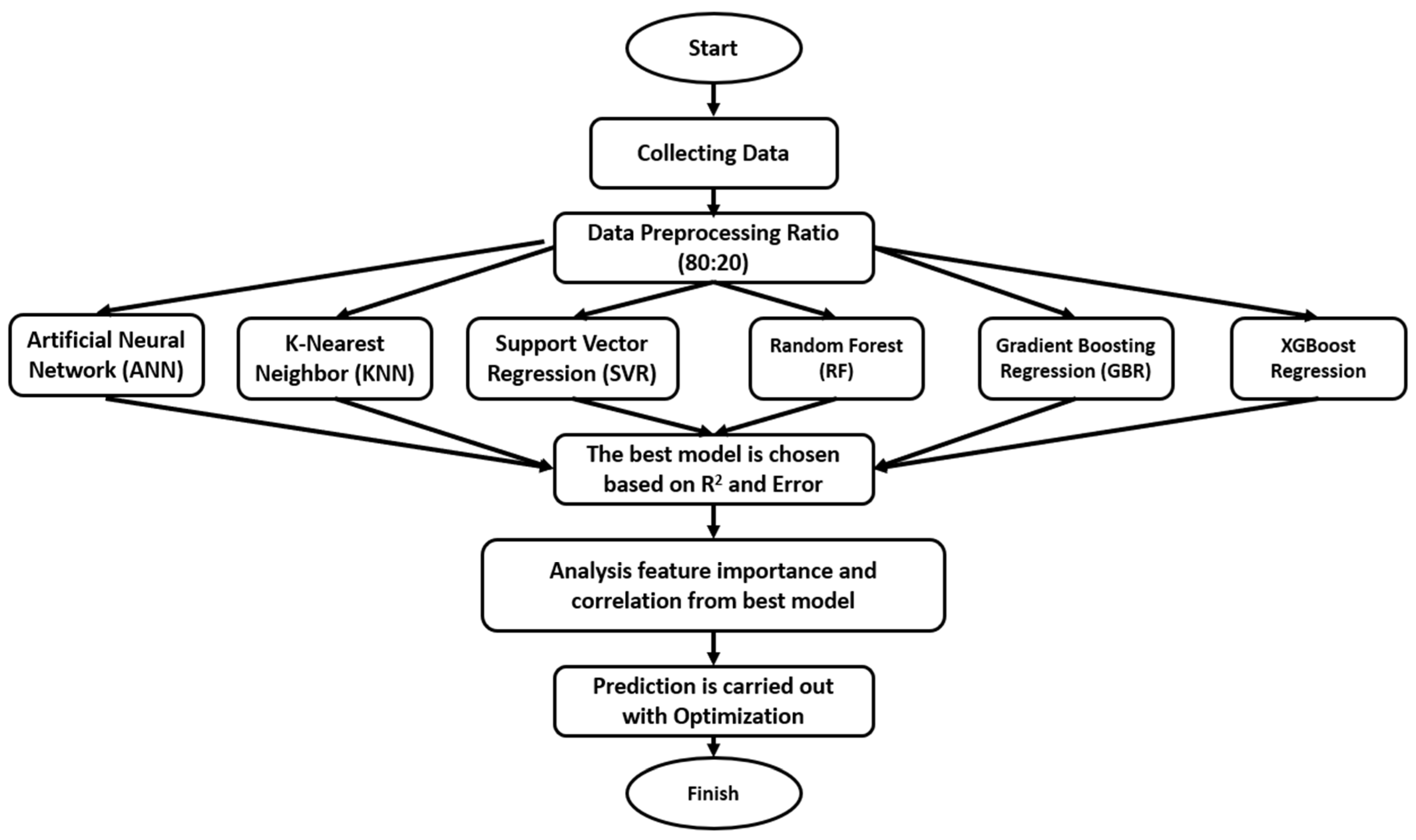
Using Google Colab, data have been divided into two exclusive sets: a training set and a test set. The training dataset serves to construct and validate the ML models, whereas the test dataset is utilized to assess the models’ performance on new data. A common data splitting approach is applied, using 80% of data (40 data points) as training for the model and 20% of data (10 data points) for testing. To avoid overfitting problems and to establish more generalized models, 5-fold cross-validation is performed. The calculated training, test and validation data are applied for predicting all responses using the established machine learning algorithms. Figure 3 demonstrates the flow chart of the present work.

2.1.1. Artificial Neural Network (ANN)

ANNs represent a category of computational systems based on the architecture and processes of the human brain. They are made up of multiple layers of interconnected neurons, which process input data and learn to recognize patterns through training. The primary components of an ANN include an input layer, several hidden layers, and a final output layer. Throughout the training process, the network modifies the weights of connections according to the prediction error, employing techniques like backpropagation. ANN is highly versatile and is capable of capturing intricate relationships within data, rendering them appropriate for various applications, including image and speech recognition, natural language processing and financial forecasting. Its ability to learn from data and improve over time enables it to perform well on tasks that involve large datasets and intricate patterns, but it requires careful tuning of hyperparameters and sufficient training data to achieve optimal performance. In Artificial Neural Networks (ANN), several parameters require optimization to enhance performance. Key parameters include the solver, which controls the weight adjustments based on the error through its line search procedure. The activation function transforms input signals and the number of hidden layers and neurons, which affects the model’s learning capacity.

2.1.2. K-Nearest Neighbor (KNN)

KNN, as indicated by its name, predicts outcomes for a new data point by referencing the closest data points (neighbors) in the training dataset. The parameter “k” specifies how many closest data points are utilized in this prediction. The parameter “n” affects the intricacy of the KNN approach, making it crucial to select an appropriate “k” based on the characteristics of data and the difficulty of the problem to optimize performance. Moreover, it is important to determine whether to apply uniform weights or weights based on proximity to the neighboring data points in the KNN model.

2.1.3. Support Vector Regression (SVR)

SVR, an extension of Support Vector Machines (SVM), is a machine learning technique designed for predicting continuous values. Unlike conventional regression approaches that focus on minimizing the discrepancy between predicted and actual outputs, SVR seeks to determine a function that closely estimates the target while maintaining a predefined margin of tolerance (ε). It ignores errors that fall within this ε-insensitive zone, focusing only on penalizing larger deviations, thereby increasing the model’s robustness [44]. The solution is constructed using only the data points that lie outside the ε margin, known as support vectors, which influence the regression line or curve. SVR can handle both linear and nonlinear relationships through the use of kernel functions like linear, polynomial, or radial basis function (RBF), allowing it to model complex patterns effectively. The performance of SVR heavily depends on the choice of hyperparameters, particularly the penalty parameter C and the kernel parameter γ.

2.1.4. Random Forest (RF)

Random Forest serves as a supervised machine learning algorithm that utilizes decision trees to gain insights based on the training dataset. It is recognized for its ability to process large datasets and address problems with a wide range of input variables effectively [45]. The RF model or algorithm is composed of a collection of individual decision trees working together as an ensemble. The predictions from these individual trees are averaged, which enhances the predictive accuracy of RF. This approach helps mitigate the issue of overfitting that can occur with simple decision trees, making RF often superior to many other machine learning algorithms. To optimize Random Forest models, key parameters that require fine-tuning include the maximum features to assess at every split (max_features) along with the number of decision trees included in an ensemble (n_estimators).
For regression, the prediction  y ^  from a Random Forest with M trees is the average of predictions from all individual decision trees  f m ( x ) :
y ^ = 1 M m = 1 M f m ( x )
where  f m ( x )  is the prediction from the m-th decision tree.

2.1.5. Gradient Boosting Regression (GBR)

GBR is a robust ensemble learning approach that constructs predictive models iteratively, with each subsequent tree trained to correct the residual errors from the preceding ones using gradient descent. This method integrates multiple weak learners—typically shallow decision trees—to form a highly effective predictive model that adeptly captures intricate nonlinear relationships [46]. GBR’s performance is largely governed by key hyperparameters: n_estimators, which determines the number of boosting iterations; learning_rate, which regulates each tree’s contribution to mitigate overfitting; max_depth, which constrains tree depth to manage complexity; and subsample, which defines the proportion of training samples utilized per tree, introducing randomness to enhance generalization.
  • The model prediction  F M   ( x )  after M iterations (trees) is:
F M   ( x ) = F 0 ( x ) + m = 1 M γ m h m ( x )
where
F0 (x) is the initial prediction (e.g., mean of y in regression);
hm (x) is the decision tree at iteration m (trained on residuals);
γm is the learning rate-adjusted weight for the m-th tree;
M is the total number of boosting iterations (trees).

2.1.6. XGBoost (Extreme Gradient Boosting)

XGBoost is an efficient and scalable implementation of gradient boosting that delivers high predictive accuracy through a combination of advanced features like regularization, parallel processing, and optimized tree-building. Like traditional Gradient Boosting Regression (GBR), XGBoost builds trees sequentially to minimize prediction errors, but it enhances performance by including both L1 (alpha) and L2 (lambda) regularization [47] to control model complexity and prevent overfitting. Its key hyperparameters include n_estimators (number of trees), learning_rate (controls the contribution of each tree), max_depth (maximum depth of trees), subsample (fraction of samples per tree), colsample_bytree (fraction of features used per tree), and gamma (minimum loss reduction required for a split). These features make XGBoost a powerful choice for regression problems in scientific and engineering applications, such as predicting mechanical or thermal responses in material datasets.
The core objective function in XGBoost includes a training loss and a regularization term as follows:
O b j = i = 1 n l ( y i ,   y ^ i ) + k = 1 K Ω ( f k )
where
  • l ( y i ,   y ^ i )  is the loss function (e.g., squared error);
  • Ω ( f k ) = γ T + 1 2 λ ω 2  is the regularization term for each tree  f k , where T is the number of leaves,  ω  is the leaf weight, and,  γ ,   λ  are regularization parameters.

2.1.7. Cross-Validation

Cross-validation is an essential method for measuring the effectiveness of machine learning models and determining their ability to adapt to new, unseen data. It is particularly useful when dealing with limited datasets, as it helps gauge how well the model performs in real-world data scenarios [48]. In K-fold cross-validation, the dataset is partitioned into random subsets, with the model being trained and validated on each subset. This approach ensures that the model is tested on different sections of the data, providing a more reliable estimate of its performance compared to a single train-test split. By using cross-validation, issues like overfitting can be detected, model parameters can be fine-tuned, and various model types can be compared. For this study, a 5-fold cross-validation approach was chosen.

2.1.8. Performance Evaluation Metrics

The model training process incorporated 5-fold cross-validation to improve generalization and reliability. The dataset was divided, with 70% allocated for training. To evaluate the models’ predictive performance, a variety of error metrics were used to compare the predicted output values with their corresponding actual measurements. These metrics included Mean Square Error (MSE), Root Mean Square Error (RMSE), Mean Absolute Error (MAE), and the Coefficient of Determination (R2). Employing multiple metrics ensured a comprehensive and balanced evaluation of each model’s accuracy. In general, smaller values of MSE, RMSE, MAE, and MAPE signify better performance, whereas an R2 value close to 1 indicates a high degree of correlation between actual and predicted outputs. The mathematical formulations of these performance indicators are outlined below:
M S E = 1 n i = 1 n ( y i y ^ i ) 2
R M S E = 1 n i = 1 n ( y i y ^ i ) 2
M A E = 1 n i = 1 n | y i y ^ i |
R 2 = 1 1 n i = 1 n ( y i y ^ i ) 2 1 n i = 1 n ( y i y ¯ ) 2

2.1.9. Optimization of Different ML Model’s Parameters

A thorough refinement of various machine learning models was carried out to achieve optimal predictive performance. The essential hyperparameters for each model were outlined previously. To optimize these parameters, a grid search method combined with 5-fold cross-validation was employed using Python 3.10 on the Google Colab platform. This approach allowed for the systematic exploration of multiple combinations of hyperparameters for each algorithm.
For the ANN model, we tuned the parameters, such as the number of neurons in hidden layers, activation functions (‘tanh’, ‘relu’), solvers (‘lbfgs’, ‘adam’), and the number of iterations. KNN was optimized by varying the number of neighbors and distance-weighting schemes (‘uniform’ and ‘distance’). SVR optimization involved adjusting the penalty parameter (C) and kernel function (‘rbf’), including tuning the gamma value. RF and GBR models were refined by changing the number of estimators, tree depth, and maximum features. In the case of XGBoost, we tuned parameters including learning rate, number of estimators, maximum tree depth, gamma, subsample ratio, and column sampling rate.
Each configuration was evaluated based on cross-validated prediction error, and the best-performing parameter set was selected to ensure strong generalization. The configurations that provided the best predictions for all the responses are documented in Table 4. Google Colab scripts were developed to implement the grid search method, which served as an additional optimization tool alongside the machine learning algorithms. By evaluating model performance across multiple parameter settings, it was aimed to minimize bias and ensure robust predictive models.

3. Results and Discussion

3.1. Model Performance Evaluation

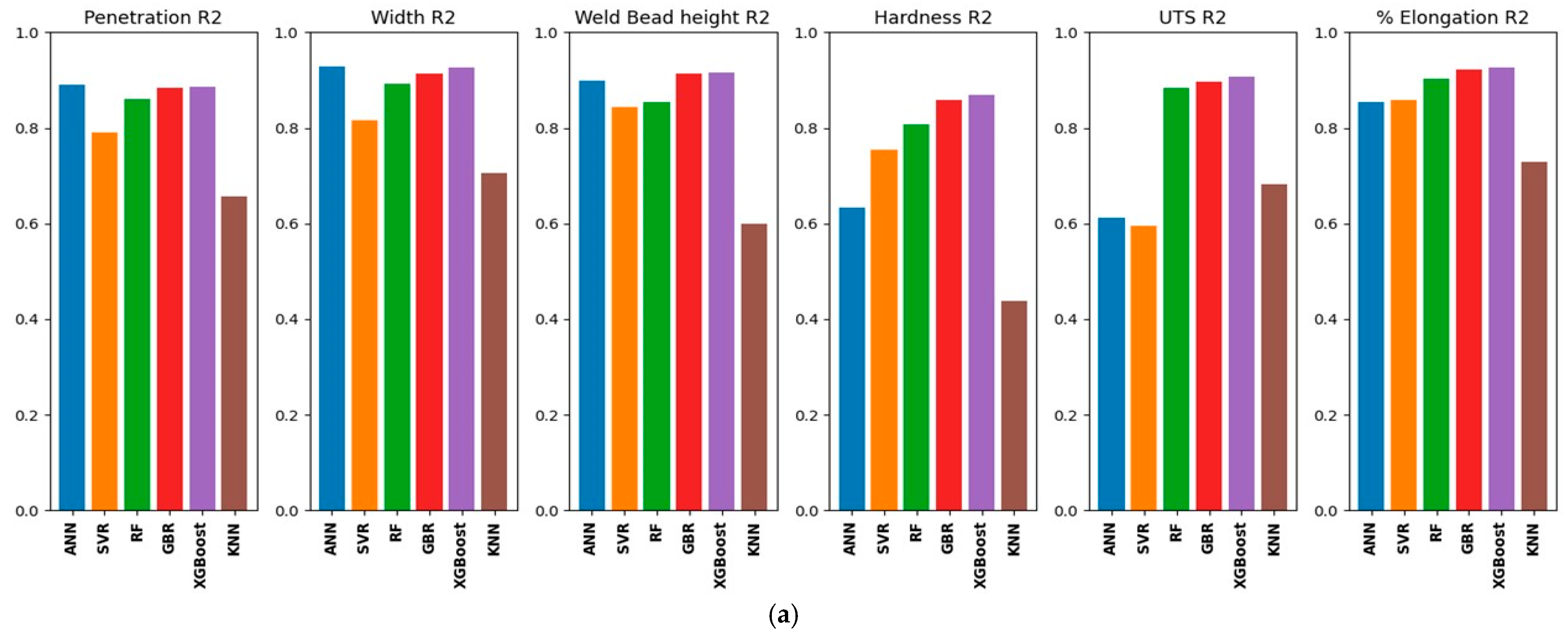
Performance metrics provide a numerical assessment of how well machine learning models correspond to actual data. In supervised learning, particularly for regression problems, the coefficient of determination (R2) is a fundamental evaluation measure. R2 reflects the fraction of variance in the dependent variable that the model successfully explains. Its value ranges from 0 to 1, where 0 indicates that the model fails to capture any variation, suggesting no predictive capability. An R2 value of less than 0.5 generally points to poor model performance. Values between 0.70 and 0.90 suggest that the model achieves a reasonably good fit, whereas values above 0.9 indicate excellent predictive performance. A perfect R2 score of 1 implies that the model accounts for all variability in the dataset without any error, although this is rarely observed with experimental data. Alongside R2, error metrics like Mean Absolute Error (MAE), Mean Squared Error (MSE), and Root Mean Squared Error (RMSE) are also critical for assessing model performance. Lower values of these errors correspond to higher model accuracy.
The bar charts represented in Figure 4a illustrate the R2 values of six machine learning models: ANN, SVM, RF, GBR, XGBoost, and KNN, and across six output parameters: penetration, width, bead height, hardness, tensile strength, and % elongation. For penetration, ANN achieves the highest R2, nearing 0.95, while KNN shows the lowest performance, at around 0.65–0.70. In predicting width and bead height, GBR and XGBoost deliver superior results, with R2 values close to 0.95, while KNN again lags. For hardness, RF, GBR, and XGBoost perform notably better, with R2 values around 0.85–0.90, whereas ANN and SVM show moderate results, and KNN remains the weakest. In tensile strength prediction, RF outperforms others with an R2 exceeding 0.90, followed closely by GBR and XGBoost, while ANN shows a relatively lower accuracy. For % elongation, all models except KNN demonstrate high R2 values above 0.85, with GBR and XGBoost slightly ahead. Overall, GBR and XGBoost consistently deliver strong predictive performance across all output parameters, while KNN shows the least effectiveness. Figure 4b represents the RMSE bar graph. For all parameters, KNN consistently shows the highest RMSE, indicating the poorest prediction accuracy. ANN and SVM exhibit higher RMSE values for penetration, width, bead height, and hardness compared to RF, GBR, and XGBoost. GBR and XGBoost models demonstrate the lowest RMSE values across almost all outputs, highlighting their superior prediction capabilities. Particularly for tensile strength and % elongation, GBR and XGBoost achieve significantly lower RMSE compared to other models. Overall, the error trends confirm that GBR and XGBoost provide more accurate predictions, while KNN performs the worst among all models. The MAE bar graph is shown in Figure 4c. Again KNN shows the highest MAE values, indicating the poorest predictive accuracy among the models. ANN and SVM also show relatively higher MAE values compared to RF, GBR, and XGBoost, particularly for hardness, tensile strength, and % elongation. GBR and XGBoost consistently achieve the lowest MAE values across all parameters, confirming their superior performance in minimizing prediction errors. Specifically, for tensile strength and % elongation, GBR and XGBoost significantly outperform the other models, with much lower error margins. Overall, this comparison highlights that GBR and XGBoost offer the most accurate predictions, while KNN yields the least reliable results. Another important performance metric is MSE, which is shown in Figure 4d. KNN shows the highest MSE values, indicating the poorest model performance with the largest prediction errors. ANN and SVM also exhibit comparatively higher MSEs than RF, GBR, and XGBoost, particularly for hardness and tensile strength. GBR and XGBoost consistently achieve the lowest MSE values across all parameters, emphasizing their strong prediction capabilities. Especially for tensile strength and % elongation, GBR and XGBoost significantly outperform the others, showcasing much smaller error magnitudes. Overall, the results demonstrate that GBR and XGBoost provide more reliable and accurate predictions, while KNN consistently underperforms. Based on the evaluation of R2, RMSE, MAE, and MSE across all output parameters, XGBoost continuously delivers the highest prediction accuracy, with higher R2 values and lower error metrics compared to other models. Both models show excellent generalization and minimal prediction errors across penetration, width, bead height, hardness, tensile strength, and % elongation. Therefore, XGBoost is identified as the best-performing model for all cases.

3.2. Feature Importance and Correlation Matrix

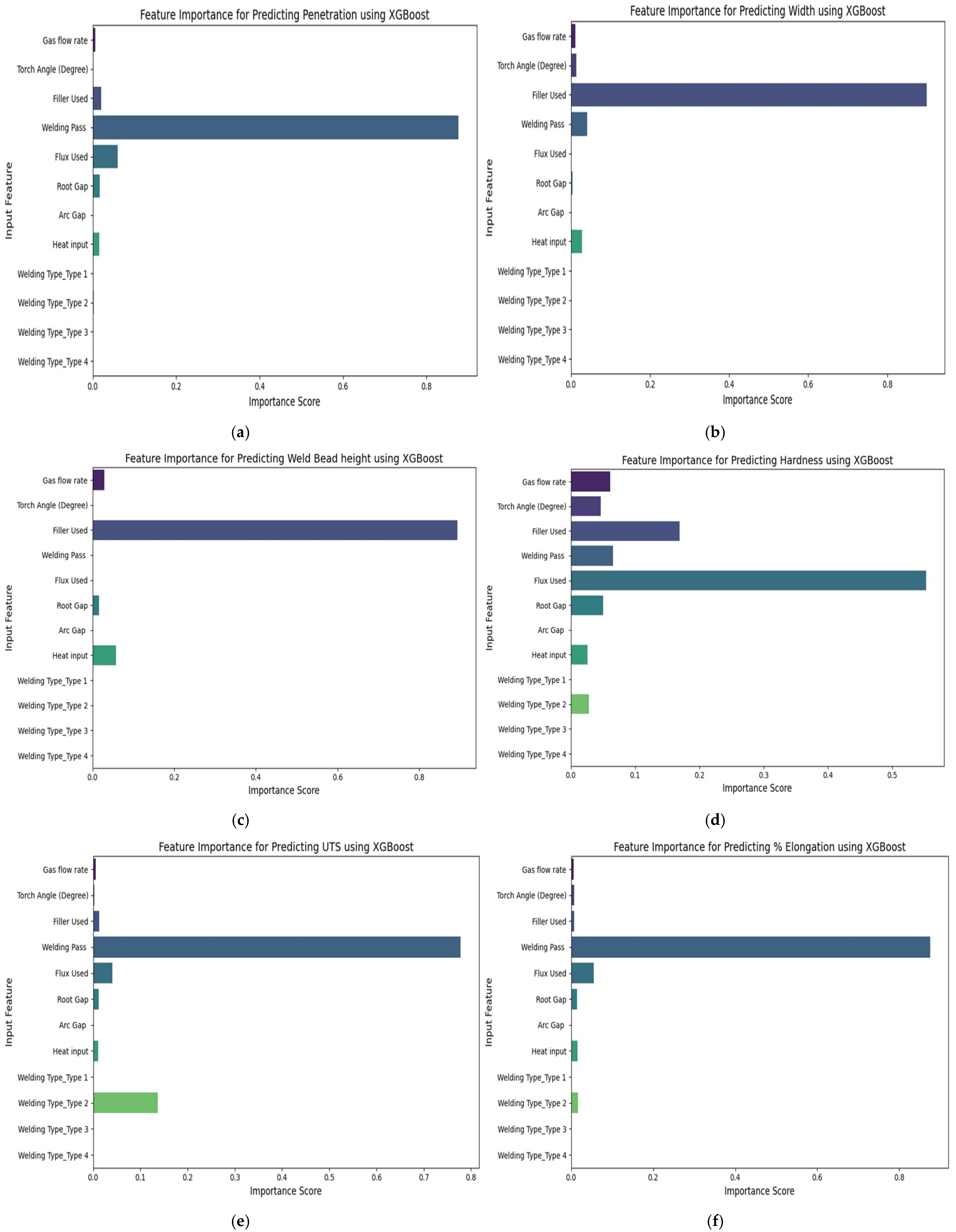
The feature importance analysis highlights the extent to which each input parameter affects the model’s output predictions. The input features considered for Feature Importance graphs are gas flow rate, torch angle, filler used, welding pass, flux used, root gap, arc gap, heat input, welding type 1 (representing Autogenous TIG on one side), welding type 2 (representing Autogenous TIG on both sides), welding type 3 (representing A-TIG welding on both sides), welding type 4 (representing filler-assisted TIG on both sides). According to the evaluation, the best-performing model is found to be XGBoost regression. A detailed breakdown of the feature’s importance is presented in Figure 5.
The feature importance analysis for predicting penetration (Figure 5a) using the XGBoost model reveals that “Welding Pass” has maximum influence, with an importance score nearing 0.9. In the present case, some experiments have been conducted with a single pass, where penetration is much smaller than the thickness of the plate. Other experiments have been carried out on both sides of the plate, meaning that two welding passes have been performed. In some of these cases, full penetration has been achieved. When single pass weld deposition is performed, the load withstanding capability of the butt-welded specimens is naturally quite smaller than the depth of penetration and hence, the area of the welded joint in these cases is considerably low. Expectedly, the strength of the welded joint is high when full penetration is achieved with weld deposition made from both sides, meaning two passes are undertaken. Considering welded butt joints, the number of welding passes is considered a parameter of the method of welding sequence. Other factors such as “Flux Used”, “Root Gap” and “Heat Input” show relatively less contribution in the present case on penetration. Parameters like “Gas Flow Rate”, “Torch Angle” and different “Welding Types” exhibit low importance scores, indicating minimal direct influence on penetration. On the whole, only when two welding passes are employed, desired full penetration has been achieved in most of the experimental runs indicating a high influence of the number of weld passes which is reflected in having a high importance score.
For predicting the weld bead width (Figure 5b), the XGBoost model identifies “Filler Used” as the dominant factor, exhibiting a significantly higher importance score compared to other variables. The application of filler material results in the spread of the molten weld pool, thereby influencing the width of the weld. “Welding Pass” and “Heat Input” contribute marginally to bead width, while parameters like “Gas Flow Rate”, “Torch Angle”, and “Welding Type” show negligible impact, indicating that bead width is primarily governed by the application of filler material.
In the case of predicting the bead height (Figure 5c), the use of filler stands out as the most critical factor within the present experimental domain, with an importance score close to 0.9. Other factors are found to have a quite low importance score, indicating their negligible influence on bead height.
For predicting hardness (Figure 5d), the use of activating flux shows the highest importance, with a score of approximately 0.54, making it the most influential factor affecting the hardness of the weld. The use of filler has the next value of importance score at around 0.18, indicating a secondary yet notable impact. “Welding Pass”, “Root Gap”, “Gas Flow Rate”, “Torch Angle” and “Heat Input” have minor effects, while “Welding Type” and “Arc Gap” show minimal contribution. This highlights that the use of activating flux influences hardness the most.
Figure 5e shows the feature importance for predicting ultimate tensile strength (UTS) using the XGBoost machine learning model. “Welding Pass” is found to be of the highest importance score (~0.77), indicating its high influence on UTS, whereas “Welding Type 2” (autogenous welding conducted on both sides) has a moderate influence on UTS. Other features like flux used and heat input show minimal impact, possibly because their effects are either secondary or already captured through other correlated variables. Overall, this analysis helps prioritize key welding parameters for optimizing UTS.
Figure 5f illustrates the feature importance for predicting percentage elongation using the XGBoost model. “Welding Pass” is observed to have a high importance score of around 0.85. When the number of welding passes is one, full penetration is never obtained in this work. On the other hand, full penetration is obtained only when welding is performed at both sides and therefore, the welded joints with more area of weld exhibit more strength and elongation. Other features like Flux Used and Welding Type 2 show minor contributions, implying that although they may influence elongation, their effects are relatively less critical compared to the welding pass. Features like gas flow rate, torch angle and heat input have negligible importance, suggesting they have a minimal direct effect on elongation in the present case.
Figure 6 is the correlation heatmap matrix illustrating the relationships between the parameters in the given dataset. The value approaching “1” signifies a strong positive relationship, meaning that when a specific feature varies, the other typically shifts expectedly: either rising or declining. The correlation value of “−1” reflects an ideal inverse relationship, wherein an enhancement in one variable directly leads to a reduction in the other. A correlation value near to “0” designates a lack of significant relationship between the variables, suggesting that variations in one do not reliably correspond to variations in the others. This heatmap shows the correlation between various input parameters (such as gas flow rate, torch angle, filler used, welding pass, flux used, root gap, arc gap and heat input) and the output responses (weld bead height, penetration, width, hardness, ultimate tensile strength and % elongation) of a welded joint. The intensity of color and correlation values (spanning from −1 to 1) illustrate both the strength and direction of relationships. Shades of red signify positive correlations, while shades of blue indicate negative correlations. White areas, on the other hand, represent weak or negligible correlation. Depth of penetration exhibits a strong positive correlation with welding pass (0.77), heat input (0.69) and flux used (0.48) indicating their significant influence on depth of penetration. More than one weld pass enables more weld deposition resulting in more area of weld joint, thereby increasing in depth of penetration. An increase in heat input increases the melt volume. When heat input increases up to a level, the depth of penetration increases and, correspondingly, UTS increases due to the higher cross-sectional area of the weld. The use of activating flux is expected to increase the depth of penetration due to the reverse Marangoni effect and constriction effect. In this case, an insulating TiO2 flux is used to coat the faying surfaces before TIG welding to obtain deeper penetration. Bead width shows positive correlations with filler used (0.76). The height of the bead has a moderate positive correlation with filler used (0.70) and heat input (0.52). Hardness is weakly correlated with most parameters but among them, flux used (0.54) has a moderate correlation. Ultimate tensile strength (UTS) shows strong positive relationships with welding pass (0.76), followed by heat input (0.73) and flux used (0.55). Similarly, % elongation shows high correlations with welding pass (0.79) and heat input (0.73).
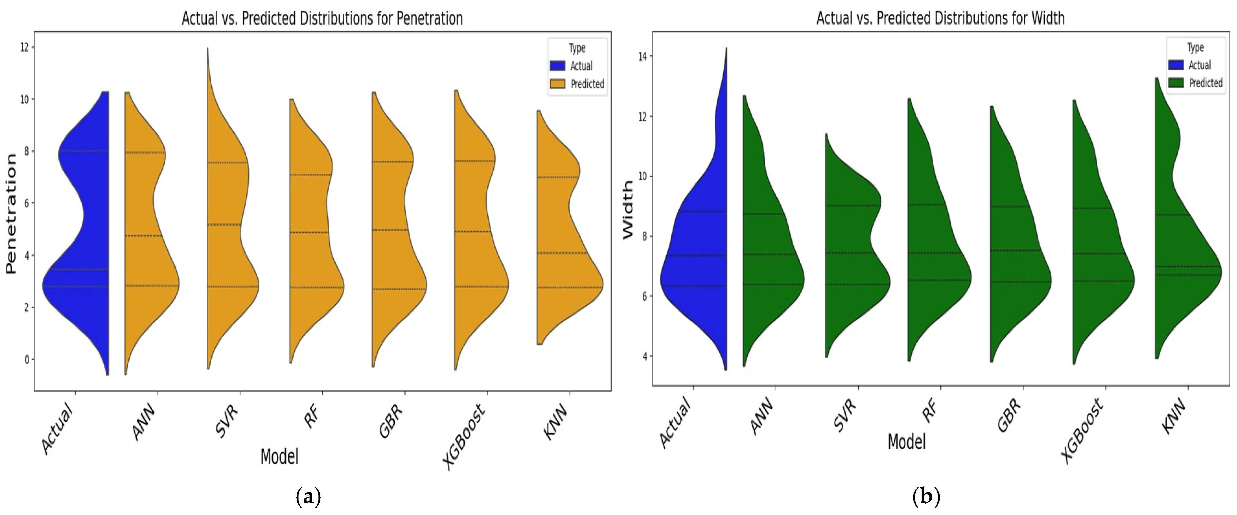
This violin plot (Figure 7a–f) shows the comparison between the actual and predicted distributions of all the outputs for various machine learning models (ANN, SVR, RF, GBR, XGBoost and KNN). The blue distribution represents the actual measured output values, while the other color distributions represent the different model predictions of different outputs. Overall, the predicted distributions closely resemble the actual distribution in shape and spread, indicating that the models can capture the general behavior of the output values. Among the models, XGBoost shows a particularly close match to the actual data, suggesting higher prediction accuracy, while slight deviations are observed in GBR, SVR, and RF predictions at the extreme values. The plot highlights that a tree-based model like XGBoost is better at mimicking the actual output behavior compared to others.

3.3. Microhardness

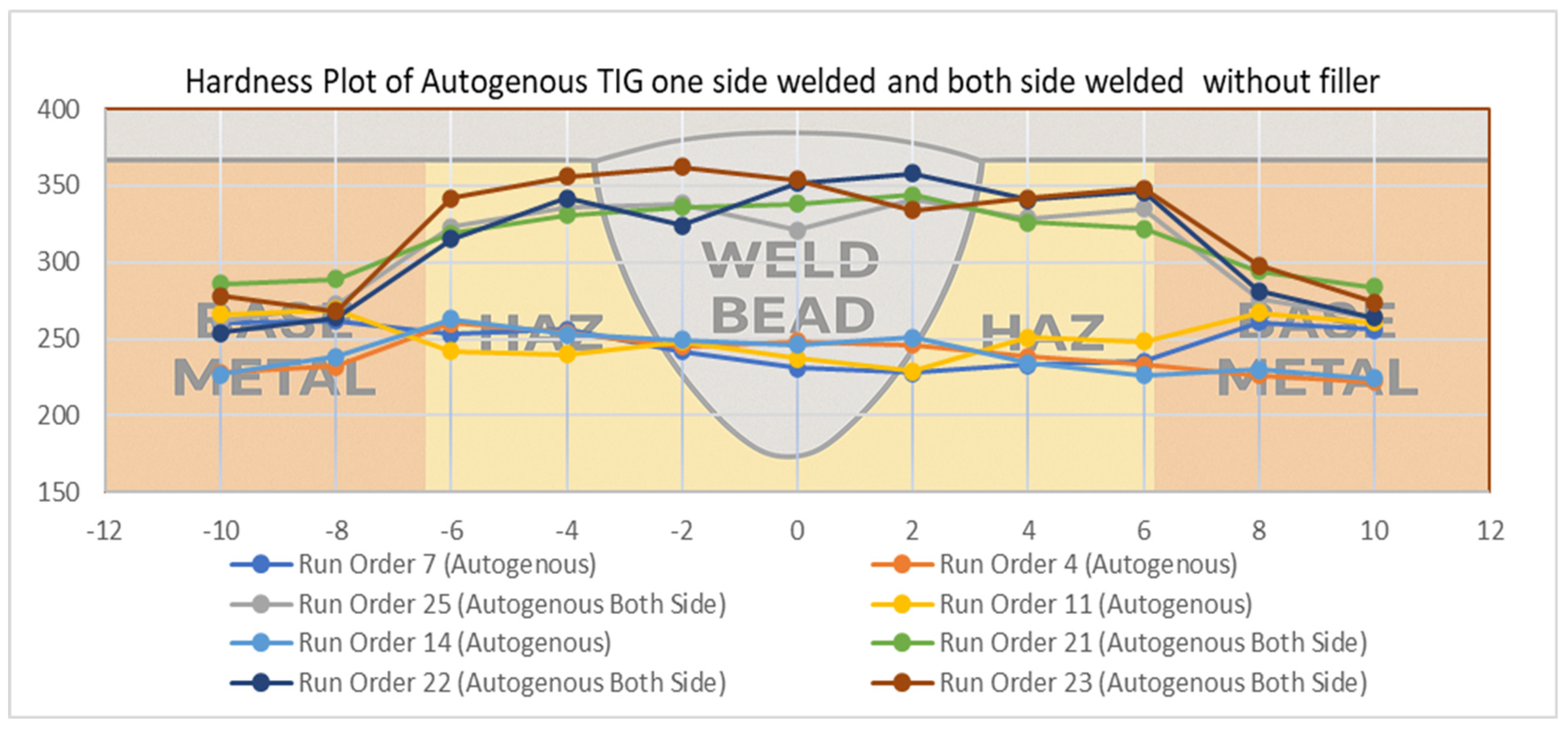
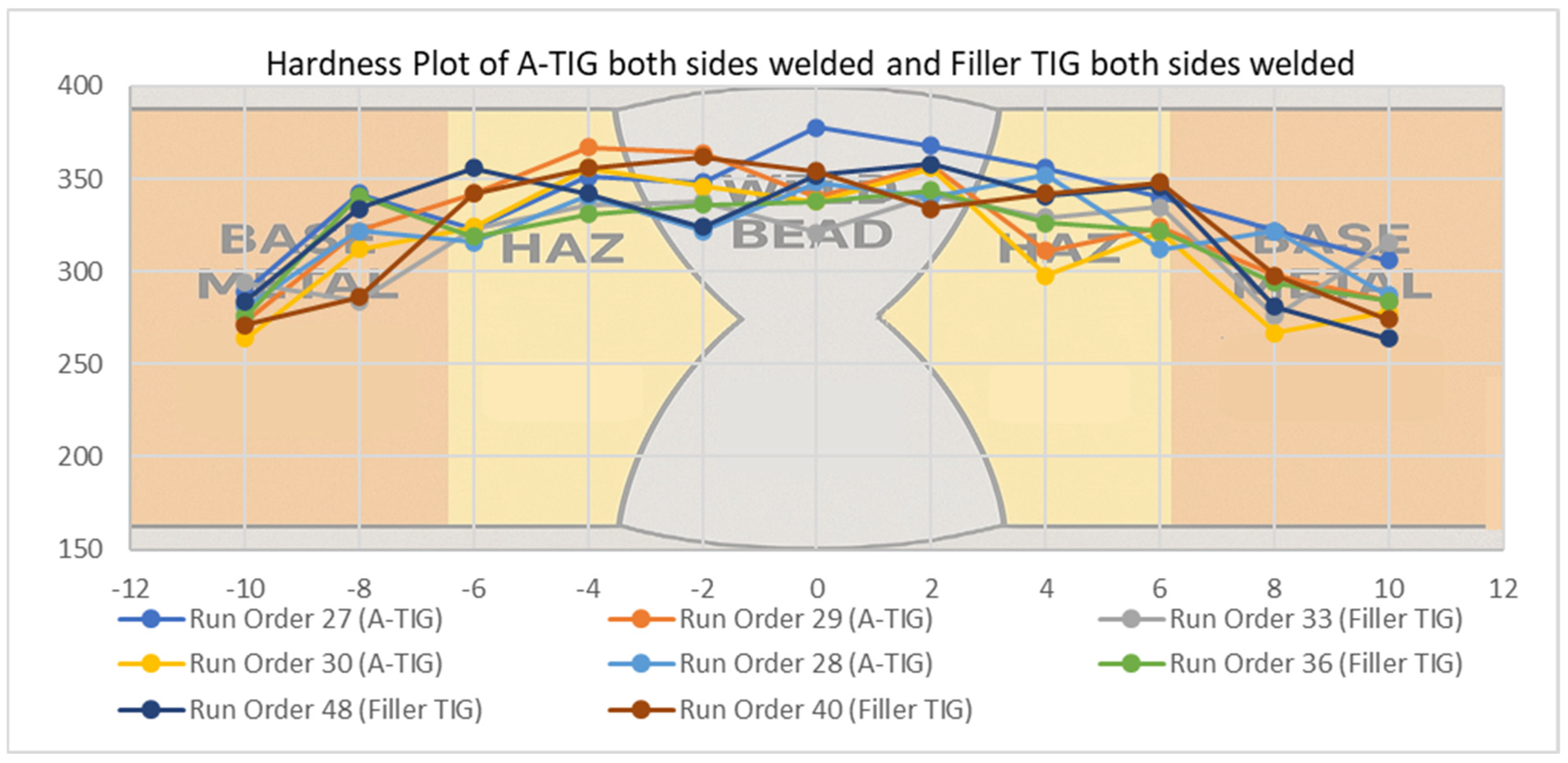
The microhardness of a few typical specimens is shown in Figure 8 and Figure 9. The figures depict the region of base metal, HAZ, and welded zone, respectively. As expected, in Figure 8, deep inside the weld pool, microhardness values are a bit low, as at this region the heat transfer rate is slow, slowing the cooling rate and lowering the microhardness values. On the other hand, a relatively high cooling rate occurs near the bead height region, making microhardness values a bit high, as in this region, the heat transfer rate is high and the cooling rate is fast, causing high microhardness. In Figure 9, compared to base material microhardness, microhardness in HAZ and weld pool is a bit high, possibly due to the high cooling rate.

3.4. Microstructure

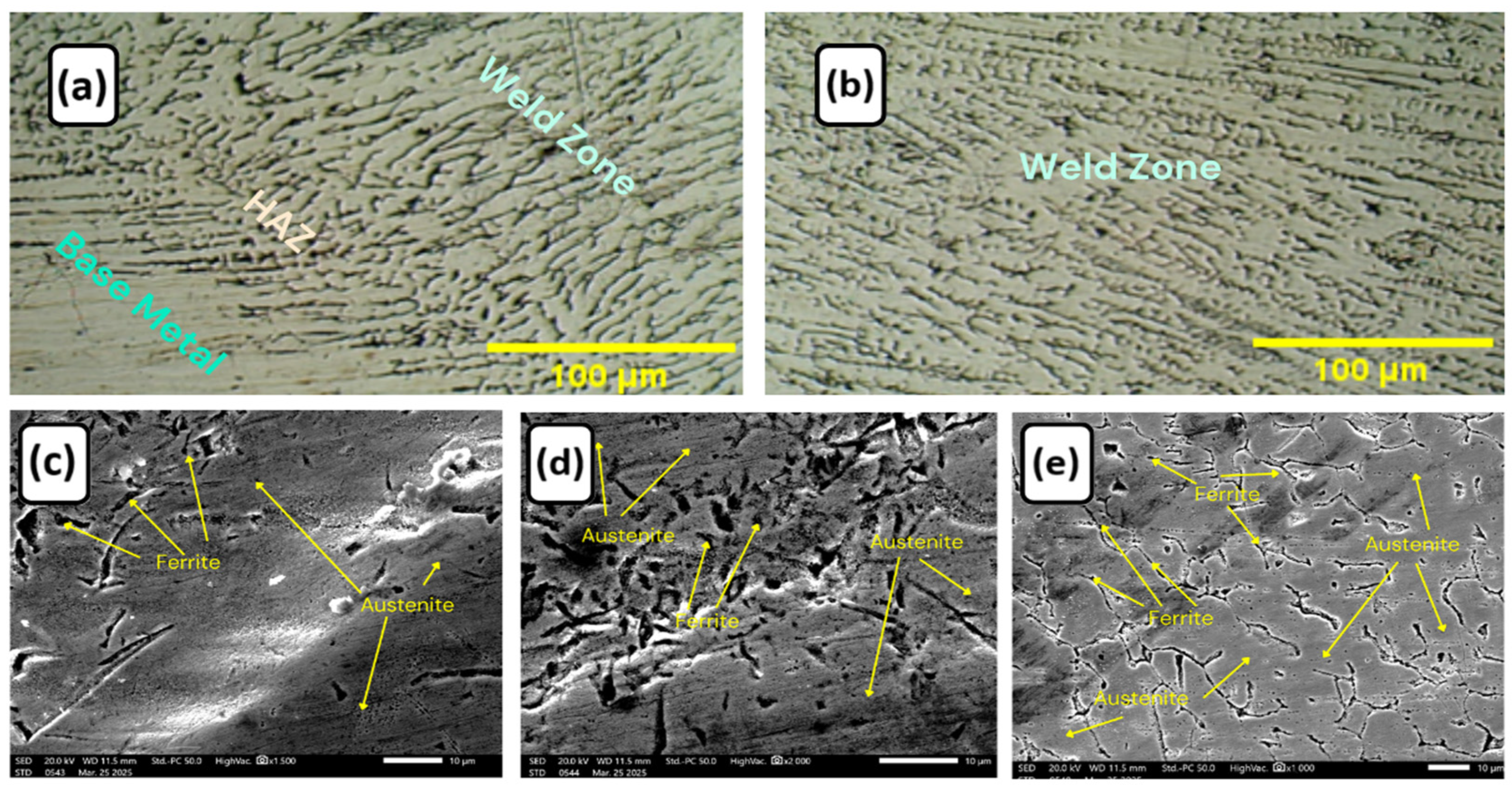
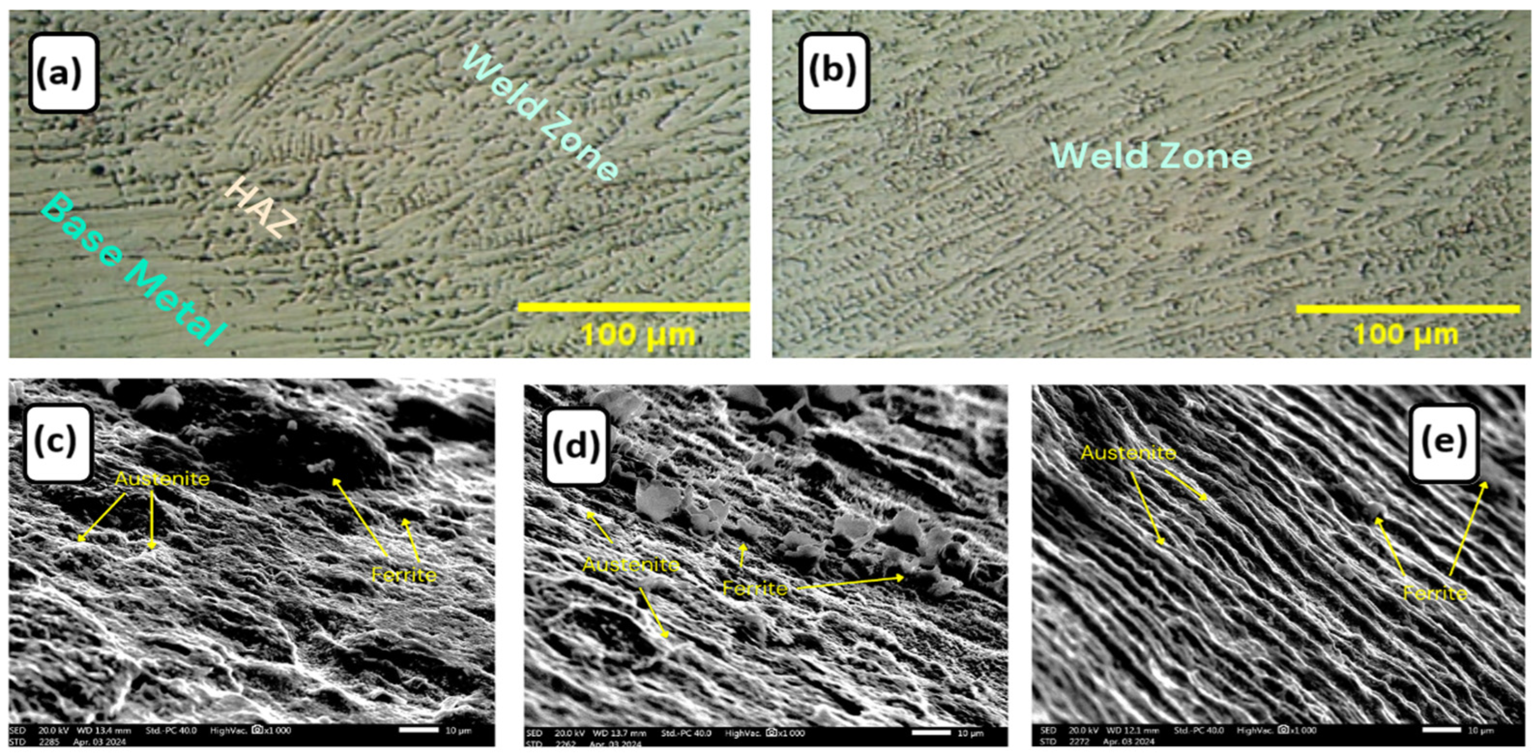
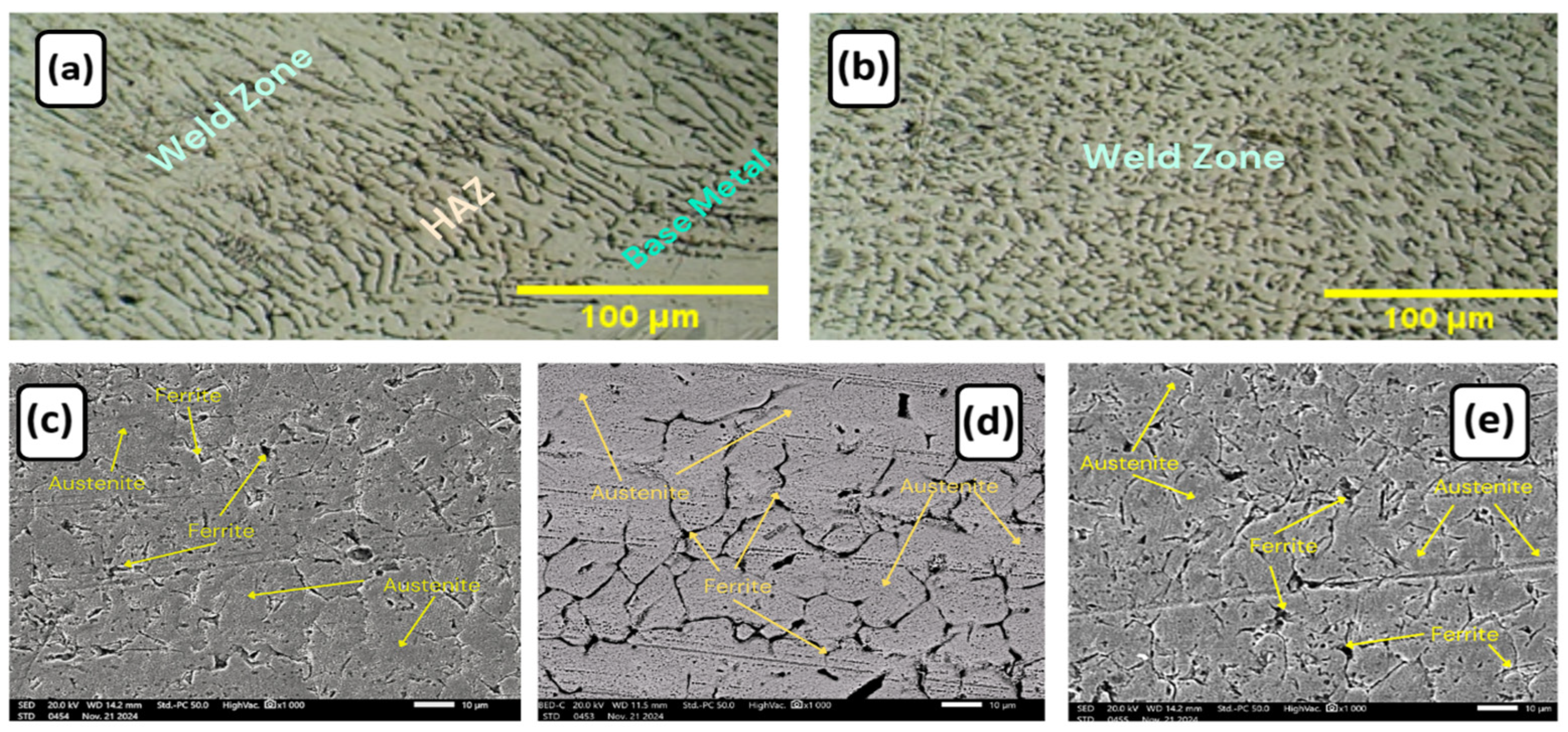
The microstructures of a few typical specimens are shown in Figure 10, Figure 11 and Figure 12. The figures depict a region of base metal, the heat-affected zone (HAZ), and the welded zone, respectively. Weld zone in this case has distinct large austenitic grain structure indicating nominal microhardness, while HAZ shows some finer grain structure giving high microhardness.
The microstructures of A-TIG weld beads using TiO2 are finer and more regular compared to other types of TIG welds where flux was not used. It can be said that TiO2 plays a major role in increasing weld penetration and grain refinement in the welding zone, also resulting in a significant improvement in welding strength.

3.5. Line EDX

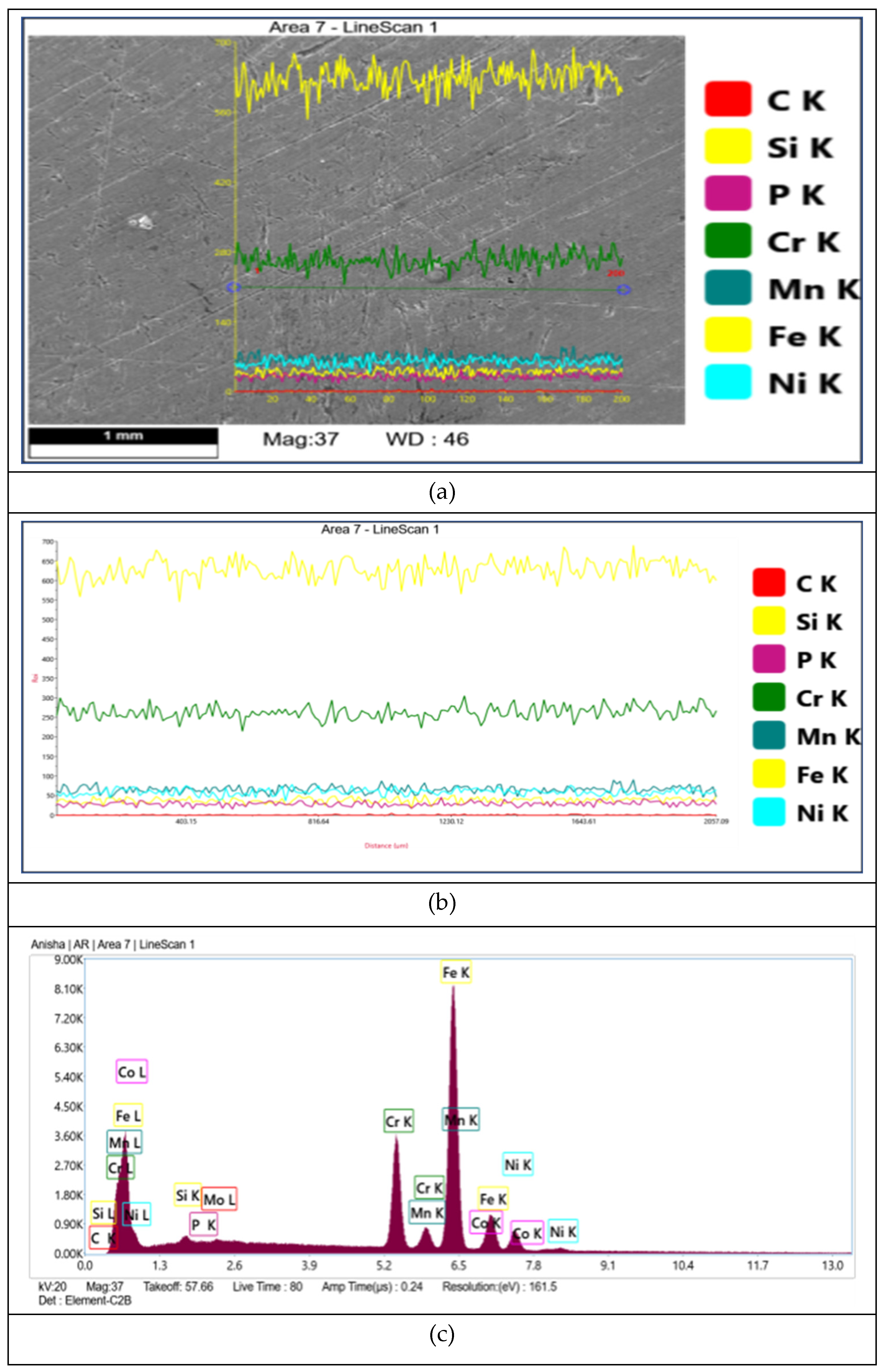
SEM micrograph of a typical A-TIG specimen is captured for EDX analysis, as shown in Figure 13. The analysis is conducted along a line traversing from the inner weld bead, across the Heat-Affected Zone (HAZ), and into the base metal, in horizontal direction.
The EDX line scan in horizontal direction of an A-TIG weld bead indicates uniform elemental intensity throughout the scanned line. Due to grain refinement in the A-TIG weld bead, no significant elemental variation was observed.

4. Conclusions

This study focused on improving the welding performance of SS304H stainless steel using TIG, Autogenous TIG and Activated TIG (A-TIG) welding techniques. In addition, machine learning models were developed to predict weld properties using eight input parameters. Based on our findings, the authors conclude the following:
  • XGBoost regression has emerged as the most effective model in predicting the welding outputs, exhibiting the highest R2 values and the lowest error rates across all responses, including penetration, width, weld bead height, hardness, ultimate tensile strength and % elongation.
  • The feature importance analysis using the XGBoost model highlights the pivotal role of specific input parameters in influencing key weld quality characteristics. Among all variables, the number of welding passes consistently emerges as the most influential factor, particularly in predicting penetration, ultimate tensile strength and percentage elongation, with importance scores nearing or exceeding 0.75. This underscores the critical role of double-sided welding in achieving full penetration and enhanced mechanical performance. The use of filler material significantly influences bead width and bead height, due to its influence on spreading molten pool and material deposition. Additionally, activating flux is identified as an impactful factor in determining weld hardness, primarily due to its role in modifying molten pool behavior through the reverse Marangoni effect, thereby improving penetration and weld quality.
  • The filler-assisted both side TIG welding also shows satisfactory results in most of the cases, achieving good mechanical properties due to full penetration.
  • Heatmap correlation analysis reveals that welding pass, heat input, and flux usage have strong positive correlations with key welding properties of the SS304H-welded joints.
  • Prediction and validation analyses confirm that the established machine learning models and in particular, XGBoost, closely match the actual experimental results across all output parameters.
  • The close alignment between predicted and experimental data highlights the effectiveness of machine learning in forecasting welding responses and optimizing process parameters.

Author Contributions

Conceptualization, S.D., B.H. and S.M.; methodology, S.S.; software, H.J.; validation, H.J.; formal analysis, H.J, B.H. and S.D.; investigation, S.S.; resources, S.D., S.M. and B.H.; data curation, S.S. and S.T.; writing—original draft preparation, S.S., H.J. and B.H.; writing—review and editing, S.D., B.H., H.J. and S.T.; visualization, S.M. and S.T.; supervision, S.D., S.M. and B.H.; project administration, B.H.; funding acquisition, B.H. and S.T. All authors have read and agreed to the published version of the manuscript.

Funding

This work was supported and funded by the Deanship of Scientific Research at Imam Mohammad Ibn Saud Islamic University (IMSIU) (grant number IMSIU-DDRSP2502).

Data Availability Statement

Data are available to all readers.

Conflicts of Interest

The authors declare no conflicts of interest.

References

  1. Habba, M.I.; Alsaleh, N.A.; Badran, T.E.; Seleman, M.M.E.-S.; Ataya, S.; EI-Nikhaily, A.E.; Abdul-Latif, A.; Ahmed, M.M.Z. Comparative study of FSW, MIG, and TIG welding of AA5083-H111 based on the evaluation of welded joints and economic aspect. Materials 2023, 16, 5124. [Google Scholar] [CrossRef] [PubMed]
  2. Kutelu, B.J.; Seidu, S.O.; Eghabor, G.I.; Ibitoye, A.I. Review of GTAW welding parameters. J. Miner. Mater. Charact. Eng. 2018, 6, 541–554. [Google Scholar] [CrossRef]
  3. Thakur, P.P.; Chapgaon, A.N. A review on effects of GTAW process parameters on weld. Int. J. Res. Appl. Sci. Eng. Technol. 2016, 4, 136–140. [Google Scholar]
  4. Pandya, D.; Badgujar, A.; Ghetiya, N. A novel perception toward welding of stainless steel by activated TIG welding: A review. Mater. Manuf. Process. 2021, 36, 877–903. [Google Scholar] [CrossRef]
  5. Kumar, K.; Sateesh Kumar, C.; Masanta, M.; Pradhan, S. A review on TIG welding technology variants and its effect on weld geometry. Mater. Today Proc. 2022, 50, 999–1004. [Google Scholar] [CrossRef]
  6. Sun, Z.; Kuo, M.; Pan, D. High deposition rate cladding by non-consumable electrode arc processes. Int. J. Mater. Prod. Technol. 2002, 17, 580–589. [Google Scholar] [CrossRef]
  7. Masuyama, F. History of power plants and progress in heat resistant steels. ISIJ Int. 2001, 41, 612–625. [Google Scholar] [CrossRef]
  8. Abe, F. Precipitate design for creep strengthening of 9% Cr tempered martensitic steel for ultra-supercritical power plants. Sci. Technol. Adv. Mater. 2008, 9, 9–15. [Google Scholar] [CrossRef]
  9. Abe, F.; Tabuchi, M. Microstructure and creep strength of welds in advanced ferritic power plant steels. Sci. Technol. Weld. Join. 2004, 9, 22–30. [Google Scholar] [CrossRef]
  10. Sourmail, T.; Bhadeshia, H.K. Microstructural evolution in two variants of NF709 at 1023 and 1073 K. Metall. Mater. Trans. A 2005, 36, 23–34. [Google Scholar] [CrossRef]
  11. Rongcan, Z.; Liying, T.; Bohan, W.; Shufang, H.; Yan, G. Effect of heat treatment on the microstructure and properties of cold-worked Inconel 740H boiler tubes. In Energy Materials; Springer: Cham, Switzerland, 2014; pp. 279–285. [Google Scholar] [CrossRef]
  12. Siefert, J.A.; Shingledecker, J.P.; DuPont, J.N.; David, S.A. Weldability and weld performance of candidate nickel based superalloys for advanced ultra-supercritical fossil power plants part II: Weldability and cross-weld creep performance. Sci. Technol. Weld. Join. 2016, 21, 397–427. [Google Scholar] [CrossRef]
  13. Shibli, I.A.; Hamata, N.L. Creep crack growth in P22 and P91 welds—Overview from SOTA and HIDA projects. Int. J. Press. Vessel. Pip. 2001, 78, 785–793. [Google Scholar] [CrossRef]
  14. David, S.A.; Siefert, J.A.; DuPont, J.N.; Shingledecker, J.P. Weldability and weld performance of candidate nickel base superalloys for advanced ultra-supercritical fossil power plants part I: Fundamentals. Sci. Technol. Weld. Join. 2015, 20, 532–552. [Google Scholar] [CrossRef]
  15. Saha, S.; Das, S.; Mondal, S. Exploring the weldability of austenitic stainless steels in advanced ultra-supercritical power plant applications: An extensive review. Indian Weld. J. 2023, 56, 54–66. [Google Scholar] [CrossRef]
  16. Sirohi, S.; Kumar, A.; Pandey, S.M.; Fydrych, D.; Kumar, S.; Pandey, C. Dissimilar autogenous TIG joint of Alloy 617 and AISI 304H steel for AUSC application. Heliyon 2023, 9, e19945. [Google Scholar] [CrossRef]
  17. Sharma, P.; Dwivedi, D.K. A-TIG welding of dissimilar P92 steel and 304H austenitic stainless steel: Mechanisms, microstructure and mechanical properties. J. Manuf. Process. 2019, 44, 166–178. [Google Scholar] [CrossRef]
  18. Thakare, J.G.; Pandey, C.; Gupta, A.; Taraphdar, P.K.; Mahapatra, M.M. Influence of microstructural heterogeneity on the mechanical performance of autogenous GTAW dissimilar joints of F/M P91 and SS304L steel. Fusion Eng. Des. 2021, 168, 112616. [Google Scholar] [CrossRef]
  19. Ogundimu, E.O.; Akinlabi, E.T.; Erinosho, M.F. Effect of welding current on mechanical properties and microstructure of TIG welding of Type-304 austenite stainless steel. J. Phys. Conf. Ser. 2019, 1378, 032022. [Google Scholar] [CrossRef]
  20. Zubairuddin, M.; Vasudevan, M.; Das, P.K.; Alam, M.M.; Kumar, K.S.; Prabhakar, S. FEM-based thermal and mechanical analysis of a comparative study of TIG and A-TIG welding on P91 steel. Sci. Rep. 2025, 15, 10271. [Google Scholar] [CrossRef]
  21. Lee, H.-K.; Yun, K.-H. A study on the applicability of A-TIG welding of semi-automatic cold wire feeding process for cryogenic stainless steel pipes. J. Weld. Join. 2024, 42, 231–238. [Google Scholar] [CrossRef]
  22. Liu, X.; Su, Y.; Zhang, G.; Wang, R.; Cai, X. Effect of longitudinal magnetic field on the microstructure and properties of A-TIG welding with different TiO2 coating amounts. Crystals 2023, 13, 66. [Google Scholar] [CrossRef]
  23. Touileb, K.; Djoudjou, R.; Hedhibi, A.C.; Ouis, A.; Benselama, A.; Ibrahim, A.; Abdo, H.S.; Samad, U.A. Comparative microstructural, mechanical, and corrosion study between dissimilar ATIG and conventional TIG weldments of 316L stainless steel and mild steel. Metals 2022, 12, 635. [Google Scholar] [CrossRef]
  24. Niagaj, J. Influence of activated fluxes on the bead shape of A-TIG welds on carbon and low-alloy steels in comparison with stainless steel AISI 304L. Metals 2021, 11, 530. [Google Scholar] [CrossRef]
  25. Saha, S.; Paul, B.C.; Das, S. Productivity improvement in butt joining of thick stainless steel plates through the usage of activated TIG welding. SN Appl. Sci. 2021, 3, 416. [Google Scholar] [CrossRef]
  26. Vidyarthy, R.S.; Dwivedi, D.K.; Muthukumaran, V. Optimization of A-TIG process parameters using response surface methodology. Mater. Manuf. Process. 2018, 33, 709–717. [Google Scholar] [CrossRef]
  27. Sharma, P.; Dwivedi, D.K. Comparative study of activated flux-GTAW and multipass-GTAW dissimilar P92 steel-304H ASS joints. Mater. Manuf. Process. 2019, 34, 1195–1204. [Google Scholar] [CrossRef]
  28. Devendranath Ramkumar, K.; Chandrasekhar, A.; Singh, A.K.; Ahuja, S.; Agarwal, A.; Arivazhagan, N.; Rabel, A.M. Comparative studies on the weldability, microstructure, and tensile properties of autogenous TIG-welded AISI 430 ferritic stainless steel with and without flux. J. Manuf. Process. 2015, 20, 54–69. [Google Scholar] [CrossRef]
  29. Ahmadi, E.; Ebrahimi, A.R. Welding of 316L austenitic stainless steel with activated tungsten inert gas process. J. Mater. Eng. Perform. 2014, 24, 1066–1073. [Google Scholar] [CrossRef]
  30. Mahajan, A.; Singh, H.; Kumar, S.; Kumar, S. Mechanical properties assessment of TIG welded SS 304 joints. Mater. Today Proc. 2022, 56, 3073–3077. [Google Scholar] [CrossRef]
  31. Rogalski, G.; Świerczyńska, A.; Landowski, M.; Fydrych, D. Mechanical and microstructural characterization of TIG welded dissimilar joints between 304L austenitic stainless steel and Incoloy 800HT nickel alloy. Metals 2020, 10, 559. [Google Scholar] [CrossRef]
  32. Rhode, M.; Erxleben, K.; Richter, T.; Schroepfer, D.; Mente, T.; Michael, T. Local mechanical properties of dissimilar metal TIG welded joints of CoCrFeMnNi high entropy alloy and AISI 304 austenitic steel. J. Mater. Sci. 2024, 59, 2623–2633. [Google Scholar] [CrossRef]
  33. Widyianto, A.; Baskoro, A.S.; Kiswanto, G. Effect of pulse currents on weld geometry and angular distortion in pulsed GTAW of 304 stainless steel butt joint. Int. J. Automot. Mech. Eng. 2020, 17, 7687–7694. [Google Scholar] [CrossRef]
  34. Ostromęcka, M.; Kolasa, A. The effect of the current pulsation frequency on heat supply results during pulsed current TIG welding in 301L stainless steel. Weld. Technol. Rev. 2019, 91, 20–26. [Google Scholar] [CrossRef]
  35. Cui, S.; Pang, S.; Pang, D.; Zhang, Z. Influence of welding speeds on the morphology, mechanical properties, and microstructure of 2205 DSS welded joint by K-TIG welding. Materials 2021, 14, 3426. [Google Scholar] [CrossRef] [PubMed]
  36. Singh, S.R.; Khanna, P. Review on A-TIG (activated flux tungsten inert gas) welding. Mater. Today Proc. 2021, 44, 808–820. [Google Scholar] [CrossRef]
  37. Khara, B.; Mandal, N.D.; Sarkar, A.; Sarkar, M.; Chakrabarti, B.; Das, S. Weld cladding with austenitic stainless steel for imparting corrosion resistance. Indian. Weld. J. 2016, 49, 74–81. [Google Scholar] [CrossRef]
  38. Saha, M.K.; Hazra, R.; Mondal, A.; Das, S. Effect of heat input on geometry of austenitic stainless steel weld bead on low carbon steel. J. Inst. Eng. (India) Ser. C 2019, 100, 607–615. [Google Scholar] [CrossRef]
  39. Mondal, A.; Saha, M.K.; Hazra, R.; Das, S. Influence of heat input on weld bead geometry using duplex stainless steel wire electrode on low alloy steel specimens. Cogent Eng. 2016, 3, 1143598. [Google Scholar] [CrossRef]
  40. Murugan, N.; Parmar, R.S.; Sud, S.K. Effect of submerged arc process variables on dilution and bead geometry in single wire surfacing. J. Mater. Process. Technol. 1993, 37, 767–780. [Google Scholar] [CrossRef]
  41. Bassey, M.O.; Ohwoekevwo, J.U.; Ikpe, A.E. Thermal analysis of AISI 1020 low carbon steel plate agglutinated by gas tungsten arc welding technique: A computational study of weld dilution using finite element method. J. Eng. Appl. Sci. 2024, 71, 33–54. [Google Scholar] [CrossRef]
  42. Saha, S.; Das, S.; Mondal, S. Experimental investigation on autogenous TIG and A-TIG welding for enhanced penetration in austenitic SS304H plates. Indian. Weld. J. 2025, 58, 75–82. [Google Scholar] [CrossRef]
  43. Singh, A.; Singh, V.; Singh, A.P.; Ashutosh, S.; Patel, D. Welding investigations on mechanical property and microstructure of TIG and A-TIG Weld of Hastelloy C-276. Eng. Res. Express 2023, 5, 025004. [Google Scholar] [CrossRef]
  44. Trinh, S.H.; Ly, H.-B. Enhancing compressive strength prediction of roller compacted concrete using machine learning techniques. Measurement 2023, 213, 113196. [Google Scholar] [CrossRef]
  45. Breiman, L. Random forests. Mach. Learn. 2001, 45, 5–32. [Google Scholar] [CrossRef]
  46. Freund, Y.; Schapire, R.E. Experiments with a new boosting algorithm. In Machine Learning, Proceedings of the Thirteenth International Conference, Bari, Italy, 3–6 July 1996; Morgan Kaufmann Publishers: San Francisco, CA, USA, 1996. [Google Scholar]
  47. Agarwal, R.; Singh, J.; Gupta, V. An intelligent approach to predict thermal injuries during orthopaedic bone drilling using machine learning. J. Braz. Soc. Mech. Sci. Eng. 2022, 44, 320. [Google Scholar] [CrossRef]
  48. Vieira, J.T.; Pereira, R.B.D.; Lauro, C.H.; Brandão, L.C.; Ferreira, J.R. Multi-objective evolutionary optimization of extreme gradient boosting regression models of the internal turning of PEEK tubes. Expert. Syst. Appl. 2024, 238, 122372. [Google Scholar] [CrossRef]
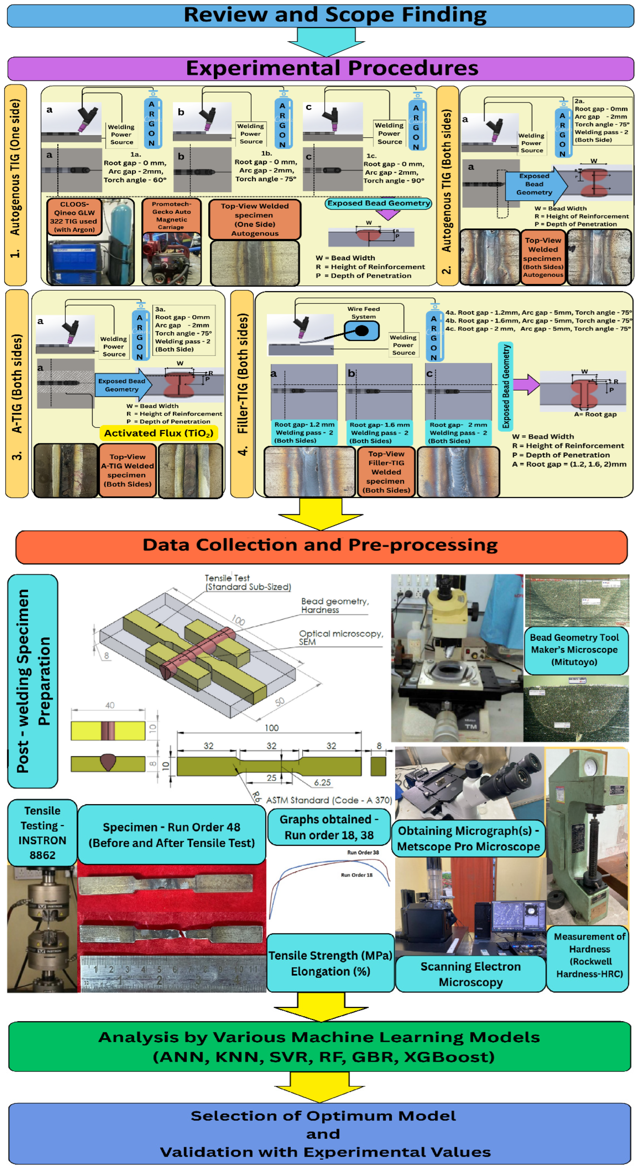
Figure 1. Present investigation process summary.
Crystals 15 00529 g001
Figure 2. Graphical presentation of regression models: (a) ANN, (b) KNN, (c) SVR, (d) RF, (e) GBM, and (f) XGBoost.
Crystals 15 00529 g002
Figure 3. Flow chart of the present work.
Crystals 15 00529 g003
Figure 4. (a). Performance metrics—R2 (Representing R2); (b) Performance metrics—RMSE; (c) Performance metrics—MAE; (d) Performance metrics—MSE.
Crystals 15 00529 g004aCrystals 15 00529 g004b
Figure 5. Feature importance of all the inputs in the XGBoost model where (a) represents Penetration, (b) represents Width, (c) represents Weld Bead height, (d) represents Hardness, (e) represents Penetration UTS, (f) represents % Elongation.
Crystals 15 00529 g005
Figure 6. Correlation heatmap matrix for XGBoost, in this Figure 6. Hyphen (-) represents minus (–) sign.
Crystals 15 00529 g006
Figure 7. Prediction and validation with actual data with different models (a) penetration, (b) width, (c) weld bead height, (d) hardness, (e) UTS, and (f) elongation.
Crystals 15 00529 g007aCrystals 15 00529 g007b
Figure 8. Microhardness plot of autogenous TIG one side welded and both sides welded without filler, in this Figure 8. Hyphen (-) represents minus (–) sign in the image.
Crystals 15 00529 g008
Figure 9. Microhardness plot of A-TIG, both sides welded, and filler TIG, both sides welded, in this Figure 9. Hyphen (-) represents minus (–) sign in the image.
Crystals 15 00529 g009
Figure 10. Microscopy of (a) base metal, HAZ, and weld bead; (b) weld bead; and (ce) SEM of weld bead of typical autogenous welded specimen.
Crystals 15 00529 g010
Figure 11. Microscopy of (a) base metal, HAZ, and weld bead; (b) weld bead; and (ce) SEM of weld bead of typical A-TIG welded specimen.
Crystals 15 00529 g011
Figure 12. Microscopy of (a) base metal, HAZ, and weld bead; (b) weld bead; and (ce) SEM of weld bead of typical filler welded specimen.
Crystals 15 00529 g012
Figure 13. Horizontal line EDX in welding zone: (a) sample overview, (b) elemental variations through line scanning, and (c) average intensity of various elements.
Crystals 15 00529 g013
Table 1. Current status of GTAW on various steel-based materials (BM).
Authors, Year, [Reference]TIG Technique and Joint Base Material (BM)Used ParametersOutcomes
Sirohi et al., 2023 [16] Autogenous TIG; IN617 alloy BM with AISI 304H steel BM (5 mm thick)Current: 200 A; Voltage: 12 V;
Travel speed: 80 mm/min; Arc length: 3 mm; Electrode angle: 60°; Shielding gas: Argon (99.99%);
Defect free welding.
Weld metal failure near AISI 304H interface and welding zone tensile strength value < AISI 304H BM and IN617 BM.
Weld fusion zone’s Mo-rich phases reduce impact characteristics; toughness ranked: AISI 304H HAZ > IN617 HAZ > weld metal.
Thakare et al., 2021 [18]Autogenous TIG;
Ferritic/Martensitic P91 BM with 304L ASS steel BM (5.6 mm thick)
Current: 240 A; Voltage: 18 V;
Arc length: 3 mm; Travel speed: 75 mm/min; Shielding gas: Argon (99.99%);
Post-weld heat treatment significantly improved the microstructure and mechanical behavior of the GTAW joint.
Ogundimu et al., 2019 [19]Autogenous TIG welding; SS 304 BM (6 mm thick) Current: 150–170 A; Shielding gas: Argon; Root height: 1 mm
Welding at a current value of 170 A produces higher tensile strength (584 MPa) and elongation (19.3%) compared to welding at 150 A.
Results indicate that higher input current leads to superior weld joints with improved mechanical properties.
Zubairuddin et al., 2025 [20]A-TIG and TIG; P91 steel BM (4 mm thick); Oxide flux Current: 110 A (TIG), 100 A (A-TIG); Voltage: 12 V (TIG), 11 V (A-TIG); Travel speed: 1.67 mm/s; Arc gap: 3 mm; Gas flow rate: 10 L/min; Torch angle: 30°
A-TIG is demonstrated in superior welds with complete penetration compared to conventional TIG in a lower heat input value.
A-TIG welding confirmed a reduction in longitudinal distortion by nearly 27% compared to conventional TIG welding.
Predictions by finite element modeling (FEM), also showed A-TIG provides better process reliability.
Lee et al., 2024 [21]A-TIG; SS STS 316L BM (4 mm thick); wire feeding (0.9 mm STS 308L; comercial STS fluxCurrent (pulse): 60–200 A; Electrode angle: 60°; Arc gap: 0.5–2.0 mm; Travel speed: 20 cm/min; Wire feeding speed: 80 cm/min; Shielding gas: Argon (99.99%) 20 L/min
The semi-automatic cold wire feeding process in A-TIG welding effectively prevents underfill and produces welds with similar tensile strength (more than 580 MPa), cryogenic impact toughness (more than 60 J) and corrosion characteristics similar to manual TIG welds in cryogenic stainless steel (STS) pipes welding.
The method was found suitable for use in cryogenic service environments.
Sharma and Dwivedi, 2023 [17]A-TIG; P92 steel BM with 304H ASS BM (8 mm thick); Flux used: Cr2O3, MoO3, SiO2 and TiO2 Current: 220 A,
Travel speed: 80 mm/min,
Arc length: 3 mm,
Shielding gas: Argon (99.99%);
Gas Flow rate: 10 L/min
Out of Cr2O3, MoO3, SiO2, and TiO2, only TiO2 enabled through-thickness penetration.
Specimens failed from 304H base metal; tensile strength: 688.6 MPa, yield strength: 562.2 MPa, elongation: 37.4%, and lower toughness (30 J) compared to the base.
Liu et al., 2023 [22]A-TIG; Mg-alloy BM (5 mm thick); TiO2 active flux coating rates: 1,2,3,4 and 5 mg/cm2Longitudinal Magnetic Field frequency: 30 Hz;
Magnetic field current: 1.5 A
Introducing a longitudinal magnetic field in the A-TIG welding process with an optimal active agent coating of 3 mg/cm2 significantly enhances the mechanical properties and quality of the welded joint by refining the grain size and reducing welding defects.
Touileb et al., 2022 [23]A-TIG; SS 316L BM with Mild Steel (MS) BM (6 mm thick);
Flux Used: SiO2, Fe2O3, Cr2O3
Current: 150 A; Travel speed: 13 cm/min; Arc length: 2.0 mm; Torch angle: 45°; Shielding gas: Pure Argon 10 L/min
Flux combination (74% SiO2, 3% Fe2O3, 13% Cr2O3, 10% NaF) in A-TIG proved high-quality welds compared to conventional TIG welding.
Single-pass A-TIG welding achieved desired depth, without edge preparation or filler metal.
Niagaj et al., 2021 [24]A-TIG; Various grades of steels (S235JR+N), P265GH, (S355J2+N), WELDOX 1300 BM (7–8 mm thickness); TiO2, SiO2, Cr2O3, NaF, AlF3 FluxesCurrent: 200 A; Voltage: 10.4–12.8 V; Travel speed: 2.5 mm/s; Shielding gas: Argon 9–10 L/min
Welding penetration increased by using fluxes TiO2 and SiO2, especially in WELDOX 1300.
Mechanical properties of A-TIG welds were comparable to or better than TIG and MAG welds.
Saha et al., (2021) [25]A-TIG; AISI-316L BM (10 mm thick); Fluxes: Cr2O3, Fe2O3, SiO2; Filler: Similar to BMCurrent: 120–150 A; Arc length: 3 mm; Travel speed: 60 mm/min; Shielding gas: Argon (99.99%) 15 L/min
SiO2 flux in A-TIG welding greatly boosted penetration depth (up to 174%) and significantly cut down welding time by nearly 70% as compared to standard TIG.
SiO2 and Fe2O3 produced smoother welds with softer fusion zones, making them preferable despite lower hardness than TIG or using Cr2O3 flux welds.
Vidyarthy et al., 2020 [26]A-TIG; 9–12% Cr Ferritic SS BM (8 mm thick)Current: 213.78 A; Travel Speed: 96.22 mm/min; Pure Argon: 10 L/min
Welding current and flux density significantly influence the depth of penetration, bead width, and depth-to-width ratio.
Increasing the welding current at high flux density leads to a more significant increase in depth of penetration and the depth-to-width ratio compared to low flux density.
Sharma and Dwivedi, 2019 [27]A-TIG and multipass TIG;
P92 steel BM with 304H ASS BM (8 mm thick); TiO2 flux;
ErNiCr-3/Inconel 82 filler
Current: 220 A; Travel speed: 80 mm/min; Arc length: 3 mm; Shielding gas: Argon (99.99%); Gas Flow rate: 10 L/min
Activated flux-GTAW using TiO2 flux enables through-thickness penetration in a single pass, reduces angular distortion, and improves tensile properties, but results in lower impact strength due to untempered martensitic structure while being more cost-effective compared to multipass-GTAW
Devendranath et al., 2015 [28]A-TIG; AISI 430 Ferritic Stainless Steel BM (5 mm thick)Current: 160–220 A; Voltage: 12.8–13.2 V (without flux), 10.2–12.2 V (with SiO2), 10.2–11.8 V (with Fe2O3); Travel speed: 75 mm/min
SiO2 helps to earn superior fusion zone hardness (225 HV) and better mechanical strength and ductility, making it ideal for achieving high-quality, single-pass welds.
SiO2 used samples maintained failure in the base metal, resulting in weldments of higher strength.
Ahmadi and Ebrahimi, 2014 [29]A-TIG; SS 316L BM; Fluxes: SiO2, TiO2, Cr2O3, CaO;
Coating Densities: 2.6, 1.3, 2.0, 7.8 mg/cm2
Current: 150 A; Travel speed: 150 mm/min; Arc length: 3 mm; Electrode angle: 60°; Shielding gas: Argon (99.99%) 12 L/min
SiO2 provided the highest depth-to-width ratio among all the used fluxes, making it the most effective in improving weld penetration.
The active element for SS316L, oxygen, at levels between 70 and 150 ppm, helped increase weld depth, while the flux-induced arc constriction boosted heat input.
Mahajan et al., 2021 [30]TIG; ASS 304 BM (6 mm thick); Fillers: ER 308L, ER 316L, and ER 310; Single V-groove (60°)Current: 150 A, 170 A; Root gap: 2.4 mm; Root face: 1.5 mm; Arc length: 3.0 mm; Shielding gas: Argon + Helium
ER 308L filler material provided superior welding properties for SS 304, including surface roughness, hardness, and tensile strength, compared to ER 316L and ER 310, despite high alloying components.
Rogalski et al., 2020 [31]TIG; 304L austenitic SS tube with Incoloy 800HT tube; Filler: S Ni 6082 Current: 60–110 A, 80–110 A; Arc Voltage: 10.5–11.0 V,
9.0–10.0 V; Travel Speed: 1.2–2.5 mm/s
TIG welding of dissimilar Incoloy 800HT and 304L stainless steel joints resulted in high tensile strength and good plasticity, with successful elimination of hot crack formation and no welding imperfections, despite initial challenges.
A reduction in hardness within the HAZ does not necessarily result in a decrease in strength, particularly for single-phase steel.
Rhode et al., 2024 [32]Pulsed-TIG; CoCrFeMnNi high entropy alloy (HEA) BM with SS AISI 304 BM (1.2 mm thick)Base current: 35 A; Peak current: 90 A; Voltage: 10 V
Pulse frequency: 4 Hz; Travel speed: 300 mm/min; Shielding gas: Argon (99.99%) 15 L/min
Defect-free dissimilar metal welds between the HEA and AISI 304 stainless steel were achieved.
Superior tensile strength of approximate value 550 MPa was achieved for both dissimilar welding.
Results confirm the mechanical compatibility of HEAs for structural applications when joined with conventional stainless steels.
Widyianto et al., 2020 [33]Pulsed TIG; SS-304 BM (3 mm thick)Current: 40 A–212 A; Travel Speed: 2.0 mm/sec; 99.99% Argon: 11 L/min 9 (upper), 3 L/min (back)
Pulsed GTAW significantly influences weld bead width and distortion, with optimal peak and base currents reducing distortion and widening the weld bead.
Ostromęcka and Kolasa (2019) [34]Pulsed-TIG; SS 301L BM (3 mm thick)Current: 140 A; Base Current (Ib): 28 A; Pulse Duty Cycle: 50%; Frequency Range: 0.5–100 Hz; Welding Speed: 2.33 mm/s; Shielding gas: Argon (99.99%) 12 L/min
The current pulse frequency in TIG welding significantly influences the welding geometry, melting efficiency, and microstructure changes in the welds and heat-affected zone, indicating a strong dependence on frequency despite constant heat input per unit length.
Cui et al., 2021 [35]Keyhole-TIG; 2205 Duplex Stainless Steel (DSS) BM
(8 mm thick)
Current: 480 A; Voltage: 16.7 V; Travel speed: 280–360 mm/min Electrode gap: 2.5 mm; Shielding gas: Argon (99.9%) 25 L/min;
Higher welding speed helped to improve ferrite content in the weld metal zone.
Microhardness and tensile strength improved with welding speed. Overall K-TIG welding produced defect-free, strong joints.
Table 2. Chemical composition of SS304H work specimen and filler wire.
ElementCSiMnPSCrNiFe
Wt.%0.0550.4771.3980.0280.0318.118.477Balance
Table 3. Experimental inputs and output parameters in this study.
Autogenous TIG Experiment Conducted on One Side
Input ParametersOutput Parameters
Run OrderGas Flow RateTorch Angle (Degree)Filler UsedWelding PassFlux UsedRoot GapArc Gap (mm)Heat Input (kJ/mm)Penetration (mm)Width (mm)Bead Height (mm)Tensile Strength (MPa)% ElongationAvg. Rockwell Hardness (HRC)
11060010020.7682.3265.932−0.1284.323.9627.67
21460010020.7682.1566.0450.00274.863.6129.67
31090010020.7681.6747.531−0.16212.621.6232.33
41490010020.7681.7356.6390.00218.671.7629
51060010021.1193.3697.869−0.14349.44.9528
61460010021.1193.0588.4220.12334.964.5831.33
71090010021.1193.4599.3750.11424.517.69630.33
81490010021.1192.9086.609−0.1346.065.2827.33
91075010020.9431.8268.2640.1206.299.23231
101475010020.9432.9246.2440.00370.221325.33
111260010020.9431.8226.0140.11231.542.2634.33
121290010020.9432.8846.4240.00351.624.3329.33
131275010020.7682.7876.5480.00328.313.7125.33
141275010021.1192.7077.1210.00332.863.7727.33
151275010020.9432.8076.311−0.19352.36428.33
161275010020.9432.6077.0290.00331.423.7629.33
171275010020.9432.7477.1620.00339.824.1731.33
181275010020.9432.9687.0080.08311.6916.78132.33
191275010020.9432.6187.1180.11326.61427.67
201275010020.9432.7126.5820.00331.424.0528.67
Autogenous TIG Experiment Conducted on Both Sides with the Best Results of the 1st set.
Input ParametersOutput Parameters
Run OrderGas flow rateTorch Angle (Degree)Filler UsedWelding PassFlux UsedRoot GapArc Gap (mm)Heat input (kJ/mm)Penetration (mm)Width (mm)Bead height (mm)Tensile Strength (MPa)% ElongationAvg. Rockwell Hardness (HRC)
211075020021.186.5305.8390.109481.7323.36828
221475020021.185.3685.590.144434.27612.67328.67
231075020021.186.0006.0660.121476.8217.56230
241475020021.185.0225.3070.00416.83411.64331.67
251275020020.9645.1746.640.177422.75412.84331.33
A− TIG Experiment Conducted on Both Sides with the Best Results of the 1st set
Input ParametersOutput Parameters
Run OrderGas flow rateTorch Angle (Degree)Filler UsedWelding PassFlux UsedRoot GapArc Gap (mm)Heat input (kJ/mm)Penetration (mm)Width (mm)Bead height (mm)Tensile Strength (MPa)% ElongationAvg. Rockwell Hardness (HRC)
261075021021.2648.0005.214−0.14648.6426.88434.33
271475021021.2648.0005.6420.00628.9426.22436.33
281075021021.2648.0005.326−0.11656.8628.34235.67
291475021021.2648.0005.8810.00636.4126.48234
301275021021.016.6406.3140.00602.08330.88732.33
Filler TIG Experiment on Both Sides
Input ParametersOutput Parameters
Run OrderGas flow rateTorch Angle (Degree)Filler UsedWelding PassFlux UsedRoot GapArc Gap (mm)Heat input (kJ/mm)Penetration (mm)Width (mm)Bead height (mm)Tensile Strength (MPa)% ElongationAvg. Rockwell Hardness (HRC)
3110751201.251.3372.8258.1051.61361.3411.34230.67
3214751201.251.3374.638.611.18468.6916.54630.33
331075120251.33788.2951.14622.24322.64329
341475120251.33787.7552.455642.53626.89233.67
3510751201.251.5288.991.315656.17231.34234.33
3614751201.251.5289.650.665634.56226.47230.67
371075120251.5289.7050.51664.23931.57327.33
381475120251.5289.1350.485676.12634.00332.33
3910751201.651.45888.321.16616.36224.34632
4014751201.651.45887.5640.621621.64324.6332
4112751201.251.4583.349.6320.34416.63116.58330
421275120251.45889.2240.56616.26323.06426.33
4312751201.651.33788.191.045618.47224.66431
4412751201.651.5288.615−0.665671.47329.37631.33
4512751201.651.4582.7311.860.69334.6826.64231.67
4612751201.651.4582.9811.8050.38346.7328.77229.33
4712751201.651.4583.2512.6150.825364.86212.56832.33
4812751201.651.45889.631.59628.0226.56830
4912751201.651.4583.4211.640.14386.79314.78230
5012751201.651.45888.890.442621.46223.84333
Table 4. Optimization parameters for all the ML models.
Model Particular Parameters
ANN1st hidden layer (8), 2nd hidden layer (8), activation = ‘tanh’, solver = ‘lbfgs’, max_iter = 10,000, random_state = 42
KNNn_neighbors = 5; weights = ‘uniform’
RFn_estimators = 100; max_features = 2, random_state = 42
SVRkernel = ‘rbf’, C = 100
GBRn_iestimators: 100; max depth: 3; learning rate: 0.1, random_state = 42
XGBoostn_estimators: 100, learning rate: 0.1, max depth: 4
Disclaimer/Publisher’s Note: The statements, opinions and data contained in all publications are solely those of the individual author(s) and contributor(s) and not of MDPI and/or the editor(s). MDPI and/or the editor(s) disclaim responsibility for any injury to people or property resulting from any ideas, methods, instructions or products referred to in the content.