An Efficient Acoustic Metamaterial Design Approach Integrating Attention Mechanisms and Autoencoder Networks

Abstract

Acoustic metamaterials have been widely applied in fields such as sound insulation and noise reduction due to their controllable band structures and unique abilities to manipulate low-frequency sound waves. However, there exists a highly nonlinear mapping relationship between their structural parameters and performance responses, which causes traditional design methods to face the problems of inefficiency and poor generalization. Therefore, this paper proposes a bidirectional modeling framework based on deep learning. We constructed a forward prediction network that integrates an attention mechanism, a multi-scale feature fusion, and a reverse design model that combines an improved autoencoder and cascaded neural network to efficiently model the dispersion performance of acoustic metamaterials. In the feedforward network, the improved forward prediction model shows superior performance compared to the traditional Convolutional Neural Network model and the model based only on the Convolutional Block Attention Module attention mechanism, with a prediction accuracy of 99.65%. It has better fitting ability and stability in the high-frequency part of the dispersion curve. In the inverse network part, compression of the high-dimensional dispersion curves by an improved autoencoder reduces the training time by about 13.5% without significant degradation of the inverse prediction accuracy. The proposed network model provides a more efficient method for the design of metamaterials.

1. Introduction

Acoustic metamaterials are a class of microstructural units that exhibit extraordinary acoustic properties through artificial design. These unconventional physical behaviors do not rely on the intrinsic properties of the constituent materials but rather stem from the artificial design of their internal architectures. Due to this unique feature, acoustic metamaterials offer remarkable design flexibility. By carefully tailoring the geometry and arrangement of their microstructures, unusual properties such as negative effective mass [1,2] and negative modulus [3] can be achieved. By utilizing these unique physical characteristics, acoustic metamaterials show great potential for applications in vibration and noise reduction [4,5], acoustic cloaking [6], and various functional acoustic devices [7,8,9,10].

Despite the rapid progress in metamaterial research, achieving on-demand design remains a critical challenge. Conventional metasurface design typically relies on iterative simulations and optimizations, representing a classic “trial-and-error” approach. As the demand grows for more complex and diverse functionalities of metamaterials, there is an urgent need to develop more efficient, flexible, and easily implementable inverse design strategies to meet the requirements for the rapid iteration and intelligent design of acoustic metamaterials for future engineering applications. Breakthroughs in artificial intelligence (AI) have provided innovative solutions to this challenge. The reverse design method based on deep learning achieves bidirectional mapping between acoustic characteristics and microstructural parameters by constructing a deep neural network (DNN) model [11,12,13,14,15,16]. Machine learning technology has demonstrated significant efficiency advantages in the design and optimization of acoustic metamaterials. Compared to traditional finite element-based iterative optimization methods, it not only reduces computation time by two or three orders of magnitude but also improves design accuracy and stability [17,18,19]. This data-driven model successfully circumvents the reliance on large-scale numerical simulations in traditional methods, marking a transformative shift in acoustic metamaterial design from experience-driven to intelligent methodologies.

The application of machine learning in the field of phononic crystals primarily focuses on predicting band structures and bandgap characteristics. Farajollahi et al. [20] used machine learning methods and artificial neural networks to predict the dispersion band gap in cylindrical acoustic metamaterials to accurately predict the relationship between the geometric parameters of cylindrical phononic crystals and their band gap ratio W. Chen et al. [21] used a CBAM attention mechanism and FPN multi-scale fusion to improve the accuracy of forward performance prediction. Hawes et al. [22] demonstrated the potential of CNN models in optimizing metamaterials for sound absorbers, providing significant noise reduction improvements with minimal material thickness. Huang et al. [18] proposed a performance prediction and reverse design method for cylindrical acoustic metamaterials based on deep learning, which can predict the upper and lower band gap limits based on input structural parameters and can quickly generate structural parameters according to the required acoustic performance. Guo et al. [23] constructed a neural network model by connecting pre-trained networks and reverse-engineered networks. The mapping relationship between the structural parameters and bandgap characteristics of acoustic metamaterials can be explored by inputting the dataset into a connected network. Early research in this area dates back to 2006, when Fuster Garcia et al. [24] combined artificial neural networks (ANN) with wavelet transform-based multiresolution analysis (MRA) to establish a mapping model between the geometric features of phononic crystals and their spectrum responses. Both numerical simulations and experimental validation demonstrated that this method could accurately predict spectrum behaviors. Regarding bandgap modulation mechanisms, Demeke et al. [25] optimized the pore structures of scatterers using composite deep neural networks. The optimized phononic crystals exhibited significantly enhanced relative bandgaps, with square and hexagonal hole structures achieving 2.382 times and 10.383 times the relative bandgap width of traditional circular holes, respectively. To address multi-dimensional parameter optimization challenges, Liu’s team [26] systematically compared the performance differences between deep backpropagation networks (DBP-NN) and radial basis function networks (RBF-NN). They found that DBP-NN is faster to train and more accurate in the single-parameter case, while RBF-NN is more stable in the multi-parameter case. Subsequently, Miao et al. [27] integrated deep neural networks with genetic algorithms (GA), and through the forward–backward retrieval process, they could design 2D phononic crystal configurations, meeting target bandgap boundaries within seconds. The average relative error of this method is only about 0.1%, which is a three-order-of-magnitude speedup compared to conventional methods. Xiao’s team [28] introduced an autoencoder-like bi-directional network architecture and incorporated a probabilistic model that greatly accelerated the inverse design of resonator-based low-frequency broadband hypersurface absorbers. These breakthroughs mark the transition of acoustic metamaterial design into a new data-driven paradigm.

To achieve the precise inverse prediction of acoustic bandgaps, Li [29] proposed a deep learning framework based on autoencoders. By coupling finite element analysis with multilayer perceptrons (MLP), they established a bidirectional “band structure-geometry” mapping model. The framework first employs autoencoders for feature encoding and the reconstruction of 2D phononic crystal structural images, then it calculates the corresponding band structure using the finite element method, and finally it transmits the extracted features to the MLP for bandgap prediction. For inverse design, simply inputting target bandgap profiles enables the MLP and decoder to collaboratively generate microstructures meeting requirements. In structural optimization, Song et al. [30] constructed a design framework for ultra-thin, ultra-light, low-frequency sound insulation metamaterials with laminated plate configurations based on deep learning. They generated large-scale training samples through finite element and acoustic impedance models, and they experimentally validated the simulation–experiment consistency, thereby achieving a high-fidelity inverse design of complex structures. Jiang et al. [31] further constructed a topology–dispersion relation deep prediction model, whose inverse design module demonstrated over 90% parameter matching accuracy in complex elastic wave manipulation. Hawes et al. [22] proposed a CNN-based inverse design framework for subwavelength microperforated panel acoustic metamaterials, which is capable of generating broadband high-absorption structures at the millisecond level while precisely controlling absorption bandwidth and amplitude at target frequencies. These studies collectively demonstrate the tremendous potential of deep learning in active bandgap regulation and the rapid design of acoustic metamaterials.

In the design of acoustic metamaterials, machine learning bypasses the complexity of traditional physical modeling by establishing the nonlinear mapping relationship between structural parameters and acoustic responses, significantly reducing the difficulty of computational design. While deep learning has a powerful nonlinear fitting capability to discover potential correlations from high-dimensional data for the accurate prediction of structural response and inverse design, its performance is still limited by the “curse of dimensionality” brought about by high-dimensional inputs, i.e., the problems of data sparsity, the dramatic increase in computational complexity, and the overfitting of models. To address this, this paper presents a study on the inverse design optimization of metasurface devices using a deep learning algorithm based on a deep neural network. The accuracy of the network can be improved by training the forward and backward networks separately. A strategy combining data dimensionality reduction algorithms with deep learning is proposed, and the input dimensions are compressed to a low-dimensional potential space by extracting key physical features in high-dimensional structural parameters (energy band curves). This strategy not only enhances the generalization ability and computational efficiency of the model by eliminating redundant information but also strengthens the exploration of physical correlations across scales through the interpretability of low-dimensional representations. Ultimately, while ensuring prediction accuracy, it significantly reduces the time and hardware costs of training and inference, providing a new approach for the efficient and intelligent design of complex acoustic metamaterials.

2. Data Preparation

Efficient data preparation forms the foundation for constructing accurate deep learning models in acoustic metamaterial design and analysis. This section details the methodology for building a multidimensional dataset encompassing microstructure topology, material parameters, and dispersion characteristics through the following two key approaches: theoretical analysis and systematic sample generation. The dataset is designed to provide robust support for subsequent forward prediction and inverse design tasks. By integrating physical principles with computational sampling strategies, we ensure that the dataset balances structural diversity, physical feasibility, and computational efficiency, enabling reliable model training and validation.

2.1. Theoretical Analysis

The dispersion curve of an acoustic metamaterial is governed by its microstructure and material parameters, which collectively establish a nonlinear mapping via the wave equation and dispersion relations. The geometric topology and material properties directly influence the energy band structure, determining the material’s ability to control acoustic wave propagation. Theoretically, the dispersion curve for a given microstructure can be derived by solving the wave equation through finite element analysis. This process yields six frequency-dependent eigenmode curves (corresponding to 31 wave vector points along the MΓXM path in the first Brillouin zone), forming a 186-dimension dataset that encapsulates the sound wave propagation characteristics. However, generating large-scale datasets through direct physical simulations presents significant challenges, including prohibitive computational costs and the incomplete exploration of the parameter space. To address these limitations, we propose systematic data generation rules that balance structural diversity with computational efficiency, ensuring physical relevance and model training feasibility.

2.2. Sample Generation

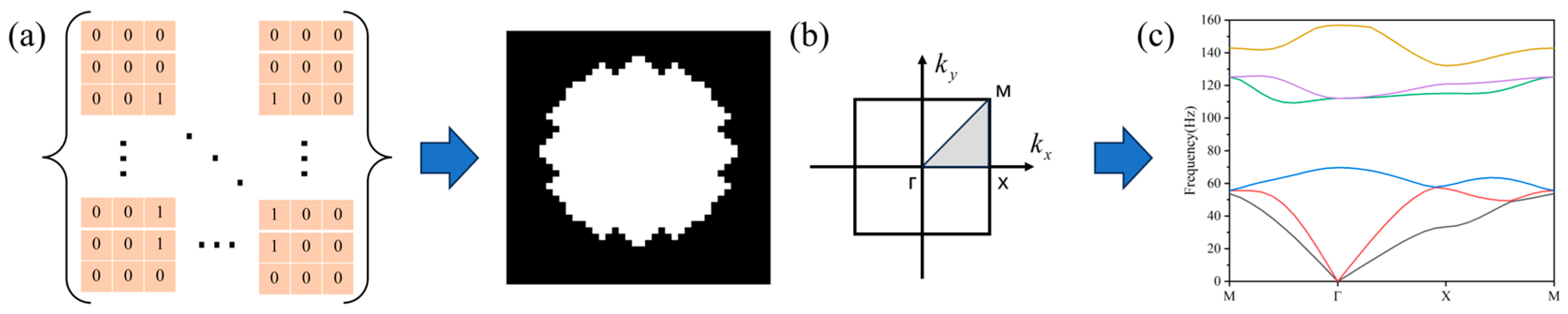
The metamaterial structure exhibits inherent spatial periodicity and symmetry. In this study, we adopt square symmetry as the lattice configuration. To ensure bandgap existence and material feasibility, the scatterer filling ratio is constrained to 0.3–0.65. Figure 1a illustrates the periodic topological structure generated via parametric curves, represented by a 40 × 40 pixel grid where black and white regions correspond to hollow and solid materials, respectively.

The shadow part of its irreducible Brillouin area, as shown in Figure 1b, is the component of the wave vector. When the finite element method is used to calculate the band structure of metamaterials, an analytical model of the single cell structure is established according to the periodicity of phononic crystals, and periodic boundary conditions are introduced by using the Bloch–Floquet theorem, which is shown as follows:

$$u(r)=e^{i\overrightarrow{k}\cdot \overrightarrow{r}}{u}_k(r)$$

(1)

where $r$ is the position vector of the local coordinate system in the cell; $u_k(r)$ is the periodic function of the position vector; $k=(k_x,k_y)$ is the wave vector. The eigenvalue problem of elastic wave propagation is transformed into the following eigenvalue equation:

$$(K-{\omega }^{2}M)U=0$$

(2)

where $\omega$ is the angular frequency of simple harmonic vibration; $K$ is the stiffness matrix of the periodic cell; $M$ is the mass matrix of the periodic cell; $U$ is a generalized displacement vector. In the process of elastic wave propagation, the continuous different wave vectors $k$ in the irreducible Brillouin zone correspond to the eigenfrequencies and eigenstates.

By scanning the wave vector $k$ along the highly symmetric point (MГXM) in the first irreducible Brillouin zone and solving the eigenfrequency, the structure of the dispersion curve can be obtained, which is in the order of 1–6 frequencies, and each frequency corresponds to 31 wave vector points, as shown in Figure 1c.

In this study, the generation of 40 × 40 binary microstructures is not entirely unconstrained “pure random”, but it introduces the following design rules to ensure the physical rationality and subsequent training effect of the samples while maintaining diversity: (1) fill factor constraint, (2) connectivity and core quantity limitation, (3) symmetry assumption, and (4) no curvature level limitation. The following text explains the specific methods of each constraint and their impact on modeling the dispersion characteristics of phononic crystals.

(1)

Fill factor constraint: In acoustic metamaterial design, range limitations are often imposed on the volume fraction of scatterers to ensure that the samples exhibit both diversity and physical significance. We restrict it to between 0.3 and 0.6 to avoid overly sparse (“ineffective” structures) or overly dense (almost whole block) conditions.

(2)

Connectivity and core quantity limitations: The designed scatterer material is distributed in a single connected domain, with each scatterer grid having at least one contact edge with other scatterer grids. The maximum height difference between each adjacent scatterer grid at the boundary between the scatterer and the substrate is one grid distance for material fabrication.

(3)

Symmetry and geometric smoothing processing: We simplified the problem, and the basic elements of the material produced are one-eighth symmetrical for ease of research. In addition, we developed a probability based material boundary formation rule. The probability of the next grid at the initial position being as high as the initial grid is p, and the probability of the next grid being lower or higher is 0.1. The position of other cells is determined by their first two cells. When the current two cells are equally high, the probability of the cell being equally high is p, and the probability of the cell being lower or higher is 0.1. When the current two cells are “low high”, the probability of this cell being one cell higher than the previous cell is p, and the probability of it being the same or lower by one cell is 0.1. When the current two cells are “high-low”, the probability of this cell being one cell lower than the previous cell is p, and the probability of it being the same or higher by one cell is 0.1.

The 20,000 sets of geometric structures and parameter combinations were generated in batches through the MATLAB R2021b program to generate data, and these topologies and simulation results are used as the basis for the training and evaluation of the deep learning models in this study. The following Formula (3) is used to uniformly perform Min–Max normalization on the image pixel values (0–1), material parameters, and frequency data to eliminate dimensional differences and improve the stability and convergence speed of model training:

$$x^{\prime }={\displaystyle \frac{x-x_{\min }}{x_{\max }-x_{\min }}}$$

(3)

where $x$ is the original data, $x_{min}$ is the minimum value of the data, $x_{max}$ is the maximum value of the data, and $x^{\prime }$ is the normalized data. All samples are packaged and stored in standard HDF5 format, and the structural images are saved as grayscale maps (40 × 40), which, together with the material parameters and dispersion eigenvectors, constitute the input data source for model training and validation.

After the data are normalized, in the prediction phase, the normalized data $x^{\prime }$ output by the model needs to be restored to the original data range through the following linear transformation:

$$y=x^{\prime }\cdot (x_{\max }-x_{\min })+x_{\min }$$

(4)

where $y$ represents the original data after normalization, $x^{\prime }$ represents the normalized data output by the model, and $x_{max}$ and $x_{min}$ are the maximum and minimum values of the training data, respectively. This normalization method ensures that, even if the model output has a small deviation (such as exceeding the range of [0, 1]), it can still be restored to a reasonable physical value through linear mapping.

3. Model Architecture

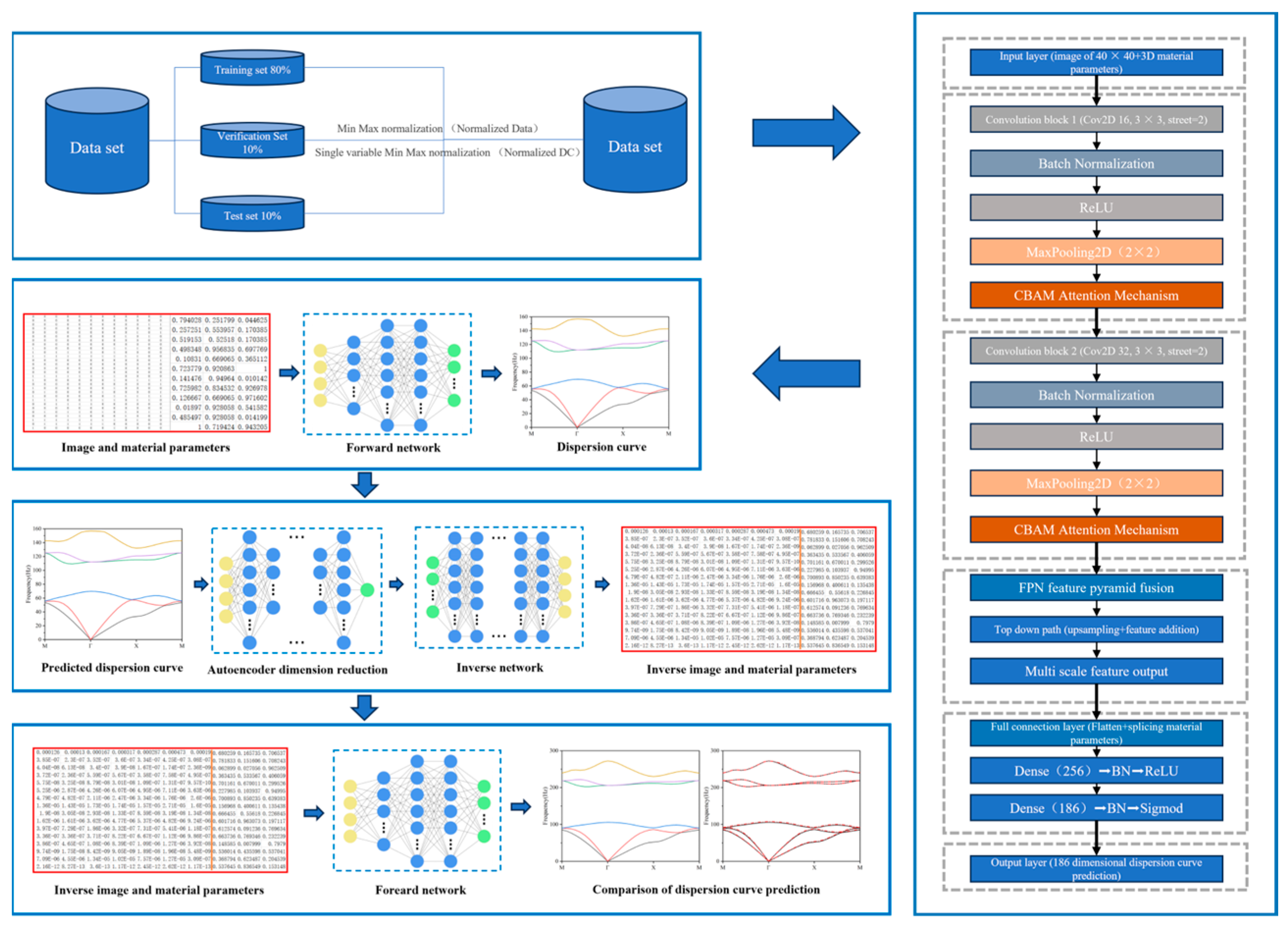
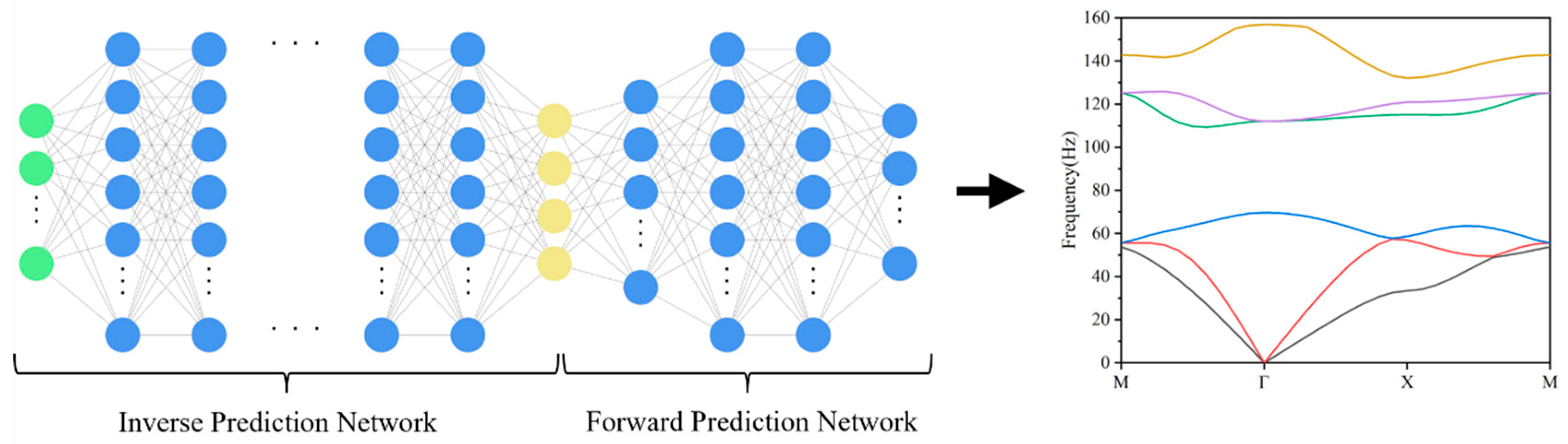
To achieve an efficient bidirectional mapping between the microstructure and dispersion characteristics of acoustic metamaterials, this study constructs a deep learning framework centered around dispersion curves for material parameter prediction and inverse design. Its overall architecture is shown in Figure 2, which consists of two parts, the forward prediction network and the inverse design network. For efficient distributed computing implementation, all neural network models in this experiment were constructed using the TensorFlow 2.11.0 framework with Python 3.7.12 development environment. The core autoencoder architecture was specifically developed through TensorFlow Keras Functional API to enable flexible model customization. All training, testing, and validation procedures were executed on a high-performance computing workstation equipped with an NVIDIA GeForce RTX 4090 GPU, operating under Ubuntu 22.04 LTS.

The forward network is based on an improved CNN architecture, integrating the CBAM attention mechanism and the FPN multi-scale feature fusion module. It is used to predict the 186-dimension dispersion curves from the material microstructure images (40 × 40) and three-dimensional material parameters (Young’s modulus, density, and Poisson’s ratio). The network extracts features through two convolutional modules; the CBAM significantly enhances the perception ability of key regions through channel and spatial attention weighting. Subsequently, the FPN module effectively integrates feature maps at different hierarchical levels through up-sampling and lateral connections, achieving the comprehensive fusion of shallow-layer detailed features and deep-layer semantic information. The final features are spread and spliced with the material parameters and mapped to the dispersion curve space through the fully connected layer. The Sigmoid function is used to constrain the output range, and the Mean Squared Error (MSE) is used as the loss function for optimization. The introduction of CBAM and FPN enables the forward network to exhibit higher fitting accuracy with better training stability in the task of multiband dispersion curve prediction, effectively alleviating the problem of difficult modeling of high-frequency modal features.

The inverse design network is based on a tandem structure of an autoencoder and TNN. The 186-dimension dispersion curve is compressed to 36 dimensions by autoencoders and then synchronized to generate 40 × 40 microscopic images and 3D parameters through a 10-layer fully connected network. A dynamic learning rate (initial 1 × 10⁻³) and batch normalization are used in training.

3.1. Forward Prediction Network

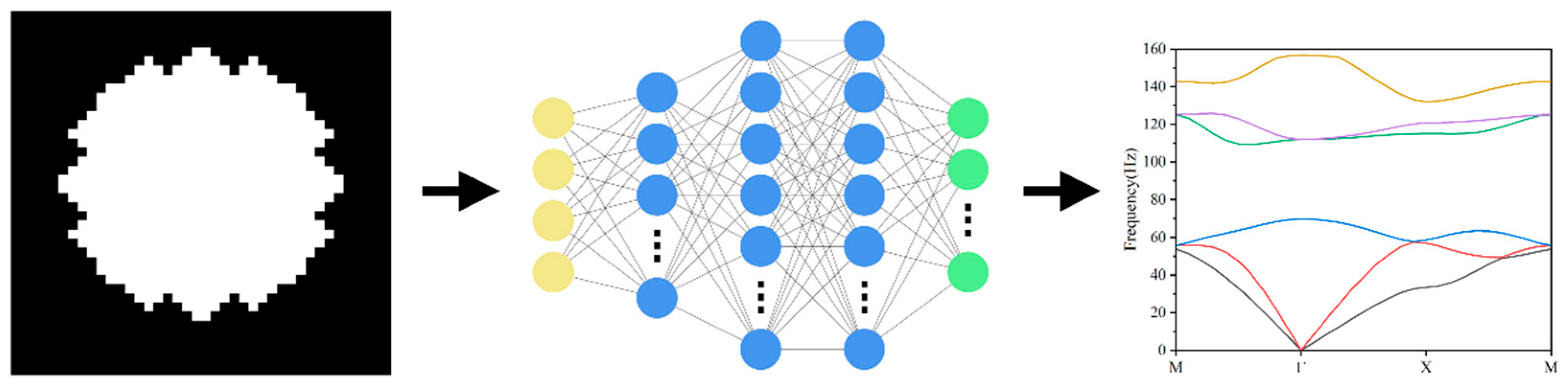
The forward prediction network is based on a Convolutional Neural Network (CNN) and incorporates the Convolutional Block Attention Module (CBAM) to enhance the model’s perception and feature selectivity of functional regions in microstructures, as shown in Figure 3. In addition to fusing feature information at different levels during the modeling process and achieving the joint modeling of local geometric details and global topological contours, the Feature Pyramid Network (FPN) structure is introduced into the network. The top-down multi-scale fusion mechanism is used to enhance the model’s ability to capture complex structure–dispersion curve mapping relationships.

The input of the network is composed of two-dimensional material microstructure images (40 × 40) and three-dimensional material parameters (Young’s modulus, density, Poisson’s ratio). The image part is feature extracted by two main convolutional modules, each of which contains a convolutional operation (Conv2D), a batch normalization (BatchNorm), an activation function (ReLU), a max pooling (MaxPooling), and a CBAM attention module to enhance the feature selection capability. In addition, the FPN top-down structure is introduced on the extracted feature maps at different levels for fusion, which further enhances the multi-scale feature modeling capability. The final output features are flattened by Flatten, spliced with the material parameters, input to the fully connected layer for nonlinear mapping, and output as 186-dimension dispersion curves. The optimization objective of the network is to minimize the MSE between the predicted dispersion curve and the true dispersion curve, as shown in the following Equation (5):

$$MSE={\displaystyle \frac{1}{q}}{\displaystyle \sum _{i=1}^q{(y_i-{\widehat{y}}_i)}^2}$$

(5)

where $q$ is the number of samples, $y_i$ is the ground truth value, and ${\hat{y}}_i$ is the predicted value. The model is trained using the Adam optimizer, with the initial learning rate set to 1 × 10⁻². Dynamic learning rate adjustment and model preservation mechanisms are used to improve the training effect and stability.

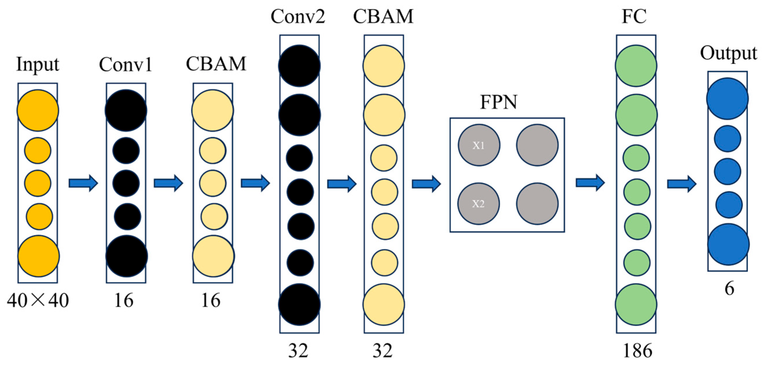
Figure 4 illustrates the functions of each main module in the forward prediction network and the corresponding number of output channels. The overall structure adopts a typical Convolutional Neural Network (CNN) as the basic framework and combines the Convolutional Block Attention Module (CBAM) attention mechanism with the Feature Pyramid Network (FPN) multi-scale fusion strategy to enhance the model’s feature perception ability.

The first layer of the network is Convolutional Block 1, which receives the input image (with a size of 40 × 40). It extracts the underlying texture and edge information through a 2D convolutional kernel, and the number of output channels is 16. Subsequently, the CBAM attention module is connected, which includes two submodules, channel attention, and spatial attention. By statistically analyzing the response intensities of the feature maps at different channels and spatial positions, the feature weights are dynamically adjusted to improve the model’s ability to recognize key structural regions. Convolutional Block 2 further deepens the network layers to capture more complex higher-order features through more sensory fields with an output channel count of 32. Similarly, a second CBAM module is connected after this layer to perform the weighted enhancement of the deeper features to increase the model’s sensitivity to the perception of the high-frequency part of the dispersion curve.

To effectively fuse information at different scales, the network introduces the FPN module to perform feature fusion on the outputs of Convolutional Block 1 and Convolutional Block 2. This module uses a top-down approach to up-sample the high-level feature maps and connect them laterally with the corresponding low-level feature maps to enhance the multi-scale modeling capability of the model. The fused feature map is flattened by the Flatten layer and concatenated with the material property parameters (Young’s modulus, density, Poisson’s ratio) to form a composite input vector that integrates the image and parameters. This vector is successively input into two fully connected layers to complete the nonlinear mapping and finally outputs a 186-dimension vector, which represents the response values of six acoustic dispersion curves at 31 wave vector points. The Sigmoid activation function is used in the last layer to ensure that the output values are within the normalized range, and the training process is optimized using the MSE as the loss function.

In summary, the network structure improves the modeling accuracy and stability of the complex nonlinear mapping relationship between microstructural features and spectral responses by introducing an attention mechanism and a multi-scale fusion strategy based on guaranteeing the modeling capability, providing a reliable means for the efficient and accurate performance prediction of acoustic metamaterials.

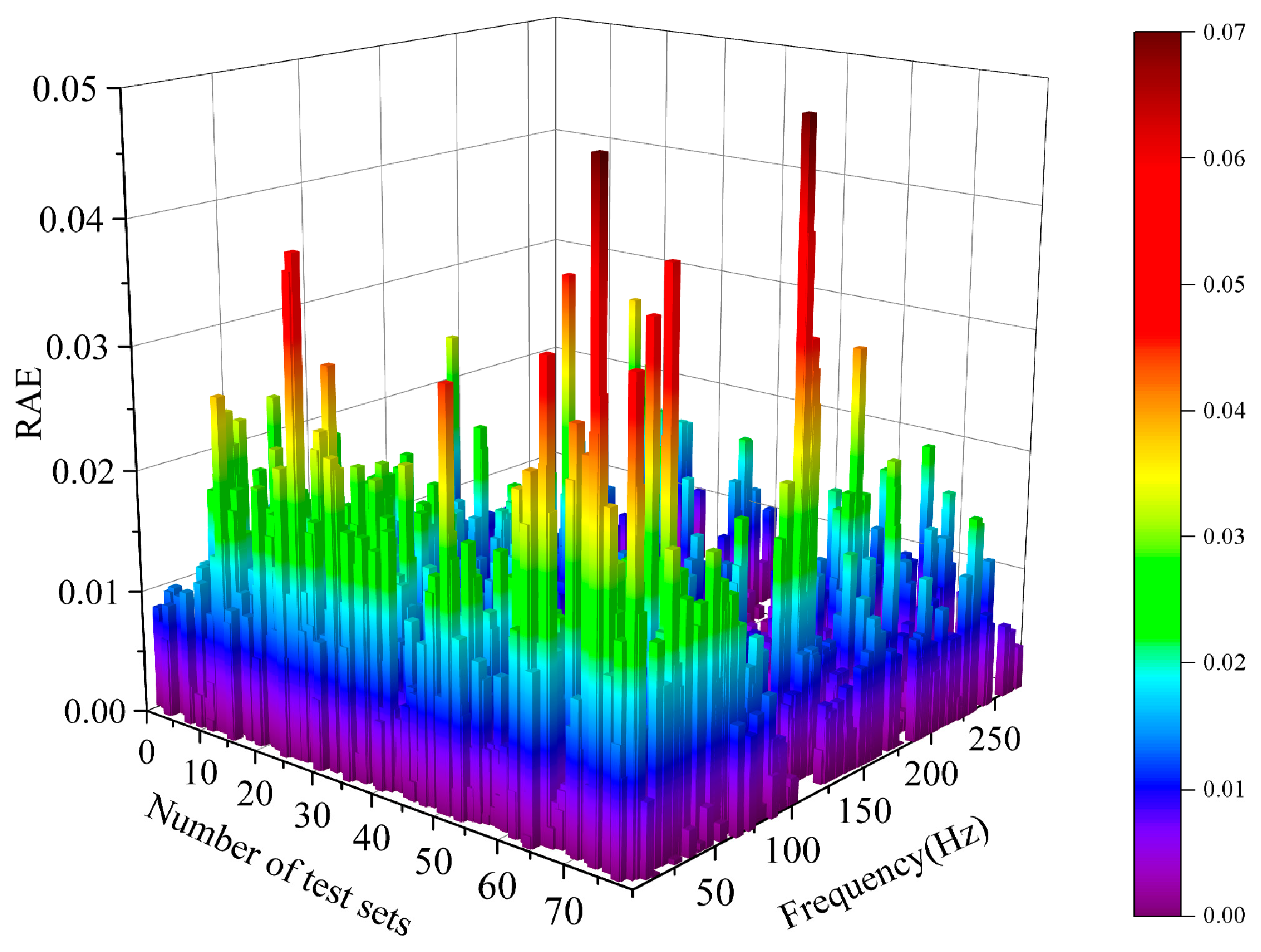
Without affecting the experimental design, we added a histogram of the relative absolute error (RAE) distribution of the dispersion curve in the forward prediction section to support the modeling progress and stability of the network structure. In the experiment, each sample had six dispersion curves with a total of 186 points. Considering the large number of samples and the similarity of sample structures, we selected 80 samples to draw their RAE histograms. The formula is shown as follows:

$$\mathrm{RAE}={\displaystyle \frac{\left|y_{\mathrm{pred}}-y_{\mathrm{true}}\right|}{y_{\mathrm{true}}}}$$

(6)

where $y_{\mathrm{pred}}$ represents the predicted value of the model, and $y_{\mathrm{true}}$ represents the true value. The histogram is shown in Figure 5.

From the diagram, it can be seen that over 95% of the samples have an RAE lower than 2 × 10⁻³, and the overall error distribution is highly concentrated. After the calculation, the average value is 0.0055, and the standard deviation is only 0.004. The high accuracy and good stability of the proposed network structure is verified in the prediction.

3.2. Inverse Prediction Network

The inverse design network aims to quickly generate the corresponding material microstructure images and material parameters based on the target dispersion curves. To improve the stability and computational efficiency of inverse design, the model introduces an improved autoencoder to downscale the high-dimensional dispersion curves and constructs an inverse neural network based on TNN.

Since the original dispersion curves are 186-dimension high-dimensional features, a symmetric autoencoder network is constructed. The autoencoder part adopts a multi-layer fully connected structure, with LeakyReLU activation and L2 regularization introduced in each layer. The decoder is reconstructed using the same number of layers and nodes, and the output layer uses the Tanh activation function. The optimization objective of the autoencoder is to minimize the MSE error between the input and the output, as shown in the following Equation (7):

$$MSE={\displaystyle \frac{1}{n}}{\displaystyle \sum _{i=1}^n{(x_i-{\widehat{x}}_i)}^2}$$

(7)

where $n$ denotes the number of samples, $x_i$ is the input of the $i$ original dispersion curve, and ${\hat{x}}_i$ is the corresponding reconstruction output of the autoencoder. After training is completed, the encoder part is extracted for a dimensionality reduction operation to compress the 186-dimension dispersion features into 36 dimensions, which are used as inputs to the inverse design model.

To recover the microscopic topology and material parameters of the metamaterials simultaneously, a tandem neural network (TNN, tandem neural network) is constructed based on the compressed variables, and its network structure is shown in Figure 5. The model body is a deep neural network composed of fully connected layer stacks, which improves training stability through batch normalization while maintaining nonlinear modeling ability. The output of the network is divided into two branches, including a 40 × 40 image output through Dense + Reshape and a three-dimensional material parameter output. The loss function is a weighted sum of the MSE for both the image and the parameters, as shown in the following Equation (8):

$$MSE=\mathsf{\alpha }MS{E}_{image}+\mathsf{\beta }MS{E}_{sp}={\displaystyle \frac{\mathsf{\alpha }}{m}}{\displaystyle \sum _{i=1}^m{(I_i-{\widehat{I}}_i)}^2}+{\displaystyle \frac{\mathsf{\beta }}{m}}{\displaystyle \sum _{i=1}^m{(s_i-{\widehat{s}}_i)}^2}$$

(8)

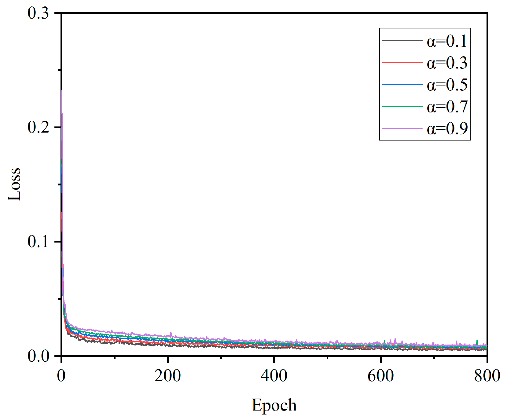
where α represents the weight of the proportion of image loss, β represents the weight of the proportion of material parameter loss, and α + β = 1. $m$ represents the number of samples, $I_i$ and ${\hat{I}}_i$ represent the real and predicted image data of the $i$ sample, respectively, and $s_i$ and ${\hat{s}}_i$ represent the real and predicted material parameters of the $i$ sample, respectively. The entire model is trained using the Adam optimizer, with 800 rounds of iteration and a batch size of 64.

From the loss function graph in Figure 6, it can be seen that the weight ratio of the two does not have a significant impact on the convergence speed during actual operation. Due to the fact that, in the process of reverse prediction, the image and material parameters of reverse prediction are used as indicators to judge the effectiveness of the reverse prediction model, we selected the same weight for the experiment, that is, α = β = 0.5. The modified formula is shown as follows in Equation (9):

$$MSE=MS{E}_{image}+MS{E}_{sp}={\displaystyle \frac{1}{m}}{\displaystyle \sum _{i=1}^m{(I_i-{\widehat{I}}_i)}^2}+{\displaystyle \frac{1}{m}}{\displaystyle \sum _{i=1}^m{(s_i-{\widehat{s}}_i)}^2}$$

(9)

After completing the model training, the dispersion curve output by the forward prediction module is compressed by the encoder and input into the TNN model for inverse generation, as shown in Figure 7. The reconstruction performance is evaluated by comparing the prediction results with the original structure and parameters. The accuracy of the inverse model in terms of image reconstruction precision and material parameter reduction is verified by evaluating the error with the original input.

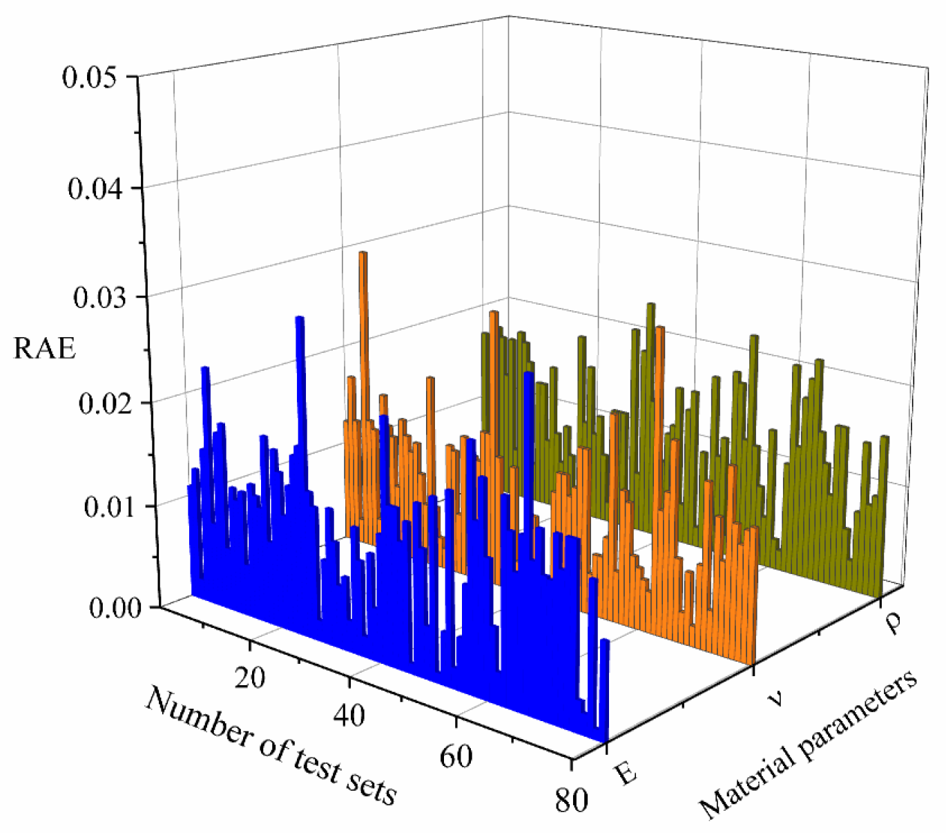
Similar to the network section, we still selected 80 validation samples without affecting the experimental design to calculate the relative absolute errors (RAE) of Young’s modulus (E), density (p), and Poisson’s ratio (v), and drew distribution histograms to demonstrate the modeling process and stability of the network structure. The histogram is shown in Figure 8.

After calculation, it was found that 95% of the samples had an RAE lower than 2 × 10⁻³, and the overall error distribution was highly concentrated, with average values of 0.004, 0.003, 0.004 and standard deviations of only 0.005, 0.002, and 0.005. This validates the high accuracy and good stability of the proposed network structure in predicting material parameters, indicating that the model has high accuracy and consistency in estimating material parameters.

4. Results

To verify the accuracy and stability of the constructed deep learning framework in the tasks of predicting the dispersion performance of materials and inverse design, this paper conducts training, testing, and comparative analysis on the forward prediction network and the inverse design network, respectively.

4.1. Forward Network Training

In the forward network pre-training network, 20,000 samples of the previously generated dataset are randomly divided into an 80% training set, a 10% validation set, and a 10% testing set. After 800 rounds of iterative training of the pre-trained network, the loss function is used to quantify the difference between the output values and the target values, which is used to reflect the training status of the CCF.

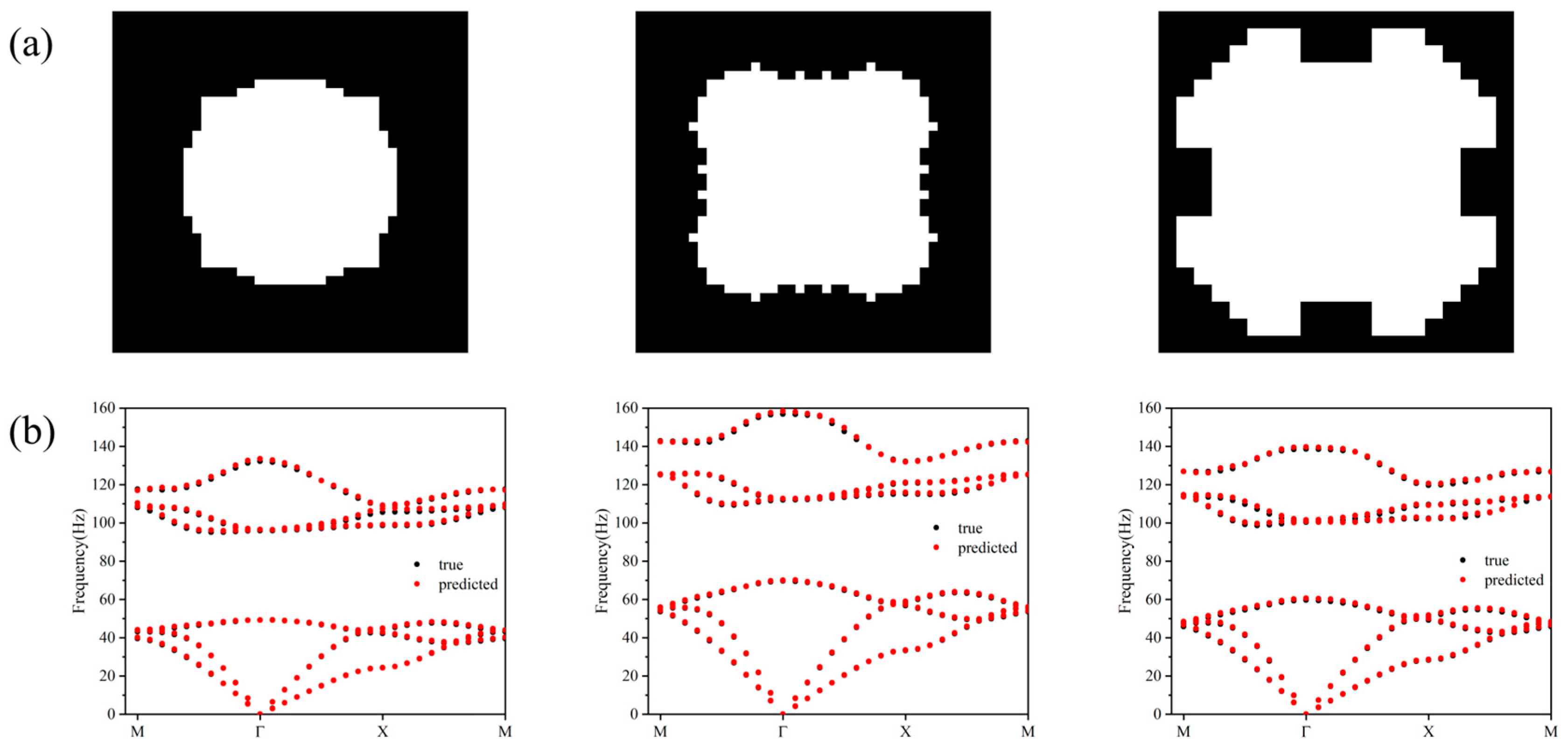
To verify the excellence of this network, we selected three materials with different filling ratios for dispersion curve prediction, and the prediction results are shown in Figure 9. Among them, the filling ratios of the three materials are 0.3, 0.4, and 0.61, respectively.

Table 1. Performance comparison of different models in dispersion prediction; all models use the following common parameters: epochs = 800, optimizer = Adam (initial learning rate 1 × 10⁻²), data sets = 20,000.

Model	Accuracy
CNN	98.73%
CC	98.43%
CCF	99.65%

gives the accuracy of the three different models under the same experimental conditions, and the prediction accuracy of the CCF model reaches 99.69%, which is better than the other two models.

To further evaluate the performance of the CCF model, the coefficient of determination $R^2$ is introduced to assess the accuracy of the model, as shown in the following Equation (10):

$$R^2=1-{\displaystyle \frac{{\displaystyle \sum _{i=1}^n{(y_i-{\widehat{y}}_i)}^2}}{{\displaystyle \sum _{i=1}^n{(y_i-\overline{y})}^2}}}$$

(10)

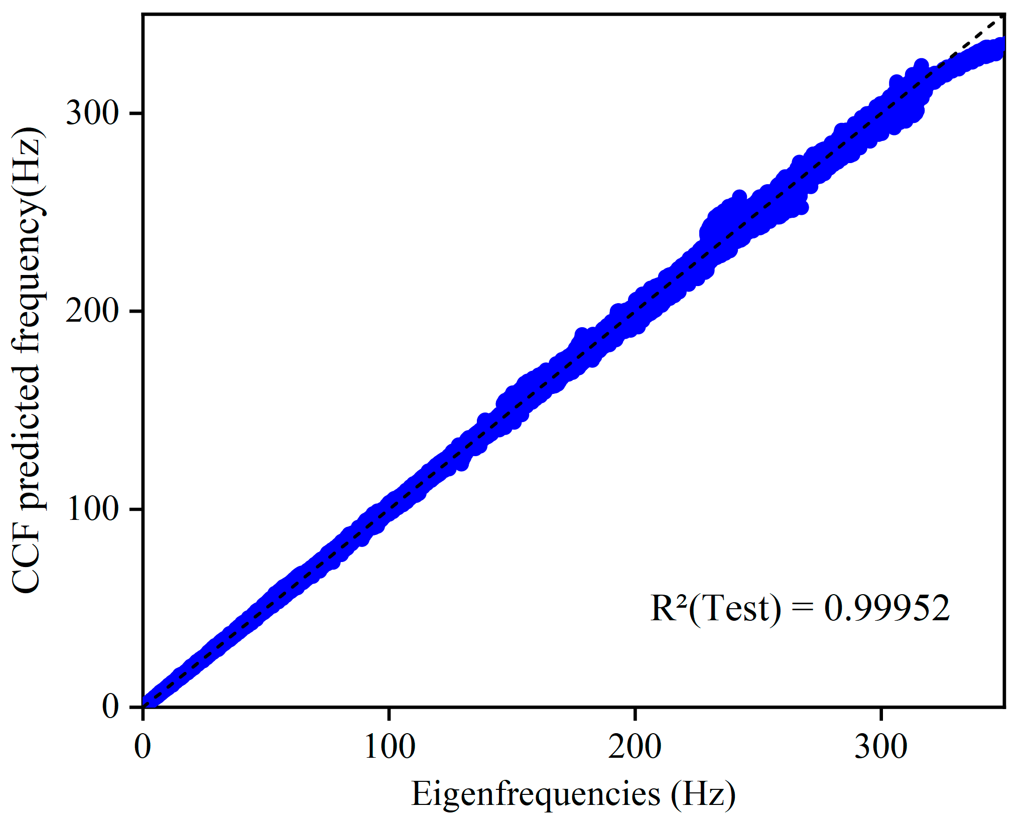
where $n$ is the number of samples in the corresponding dataset, $y_i$ and ${\hat{y}}_i$ are the true and predicted values of the $ith$ sample, and $\overline{y}$ is the average of the true values. Figure 10 shows the comparison between the predicted and true values of the dispersion curves of the forward design network of the CCF model during the testing process. It can be seen that the data points are all distributed near the dotted line, and the values of the coefficient of determination are all higher than 0.99, which indicates that there is a very good agreement between the true and predicted values. The overall performance shows that the CCF network can accurately predict the dispersion relation of acoustic metamaterials.

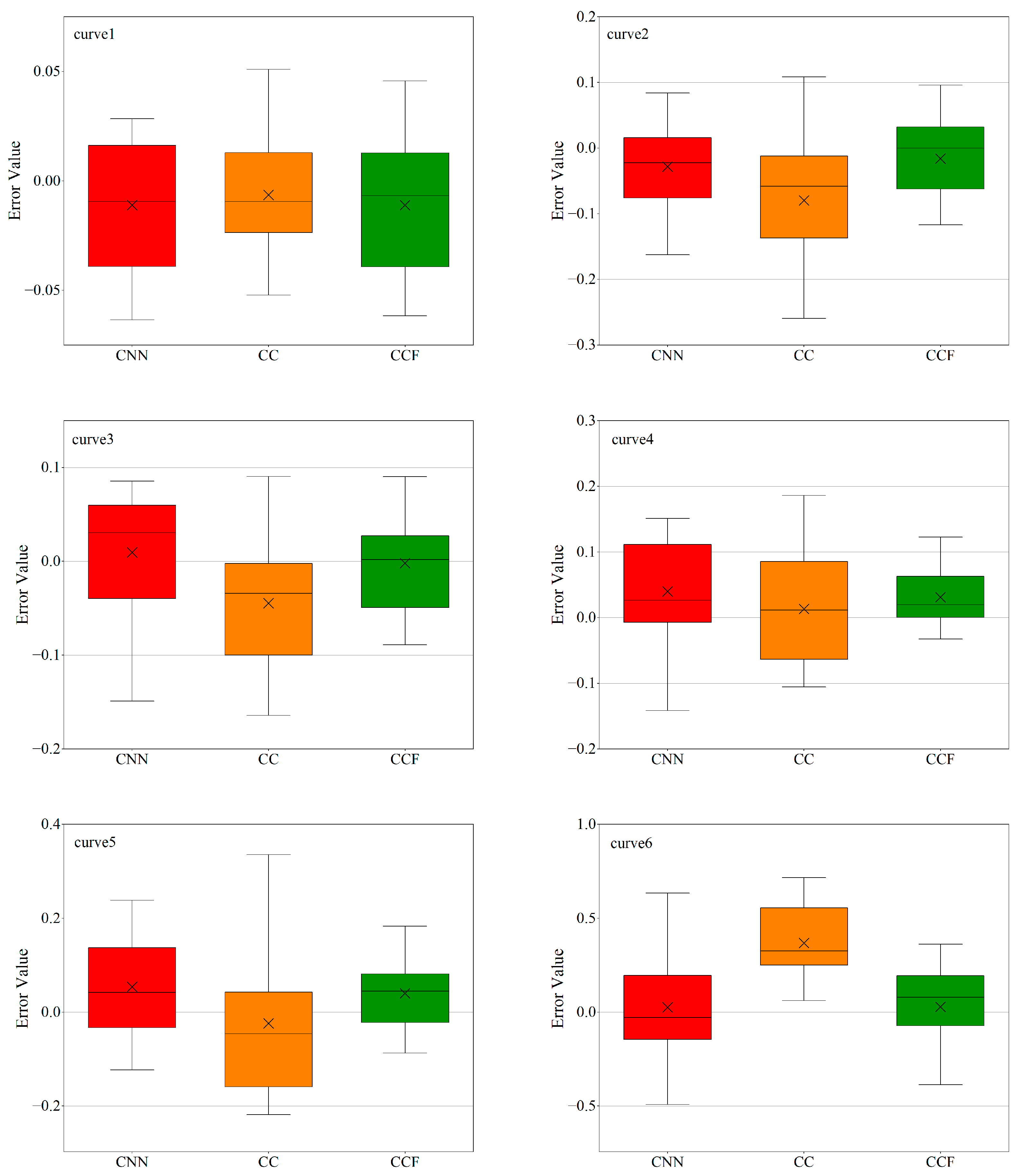
To better analyze the advantages of the CCF model among these three models, Figure 11 shows the box plots of the prediction error distributions of the three network models (CNN, CC, and CCF) on the test set, which reflect the performance stability and overall prediction ability of each model in multiple experiments. The box plots include the maximum value, minimum value, median, and the upper and lower quartiles of the errors during the training process of the models. There are no outliers in the prediction results of the three models, which conveys a positive signal. This means that the quality of the dataset is high, and the error values obtained by each model are statistically relatively uniform without extreme error values, ensuring the fairness of the comparison of these models.

To thoroughly analyze model performance across different dispersion frequencies, we present box plots comparing the prediction errors of CNN, CC (CNN_CBAM), and CCF models on six dispersion curves (curve 1–curve 6, ordered from low to high frequency). Specifically, we use the error values between predicted and actual dispersion curves as evaluation parameters, and the results are shown in Figure 11. For the low-frequency dominant curve 1, all three models exhibit compact error distributions. However, the median error of the CCF model is about 0.00673, which is better than the other two algorithms, whose median errors are 0.00937 and 0.00938, respectively. CCF also shows similar performance advantages on curves 2 and 3, indicating that it has better overall quality, accuracy, and stability in low-frequency prediction. When reaching curve 4, prediction errors increase across all models with more pronounced performance variations. The CCF model maintains lower median errors, with an interquartile range (IQR) of 0.06291 compared to 0.11859 and 0.91740 for the other models. This performance advantage persists across curves 5–6. This shows that the CCF model produces the least dispersion of error in predicting high-frequency dispersion curves, indicating that this model is robust and adaptable to data with different frequency characteristics.

Based on this analysis, the CCF model surpasses both CNN and CC models in forward prediction accuracy, particularly demonstrating enhanced performance in high-frequency predictions. These results substantiate CCF’s strong stability and robustness.

4.2. Inverse Network Training

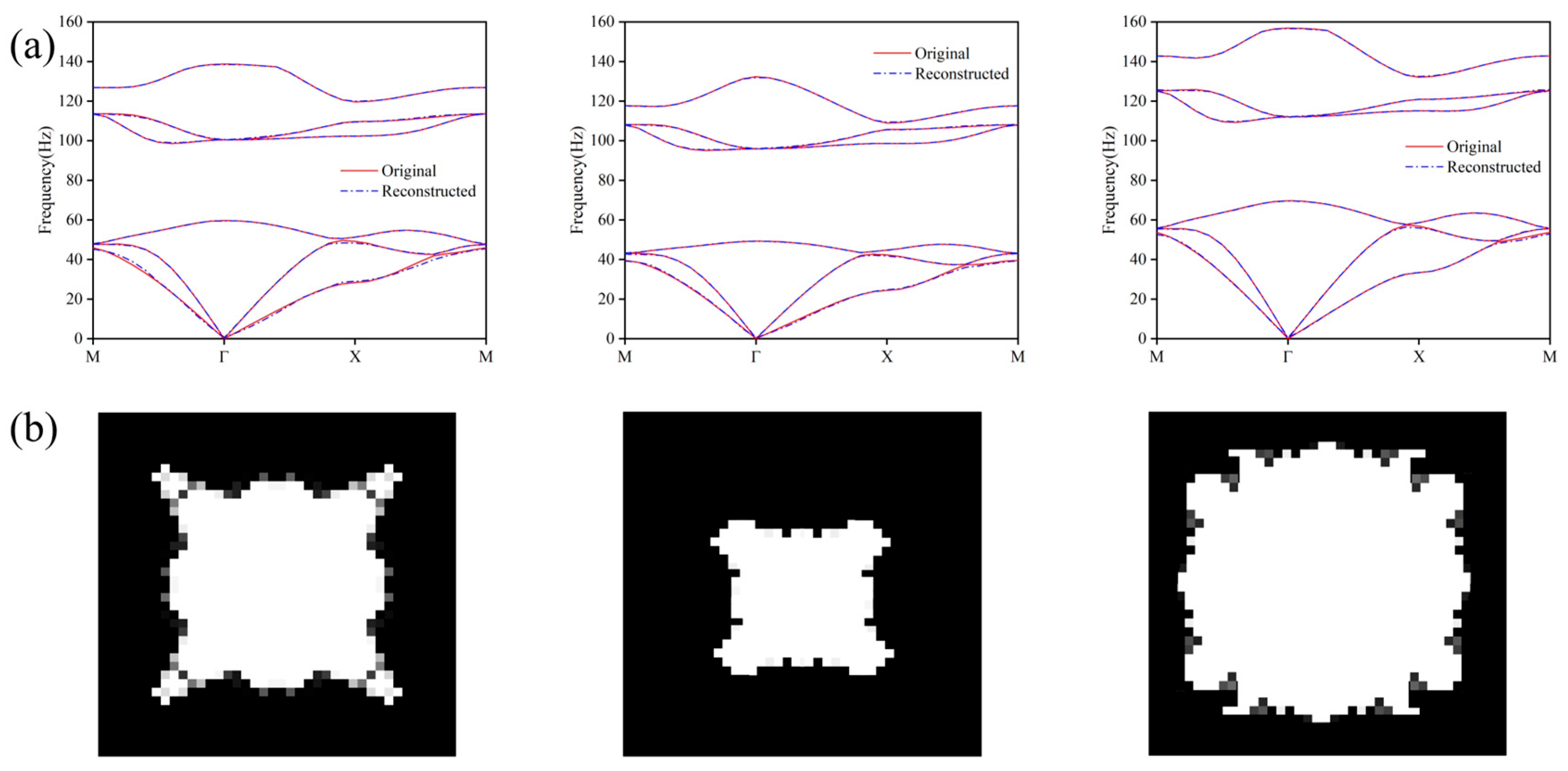
To address the curse of the dimensionality problem brought by high-dimensional dispersion data in inverse design, this paper uses an autoencoder structure to reduce the dimensionality of the dispersion curves obtained from forward prediction. The encoder adopts a symmetric structure, with 50 training rounds, and an early stopping mechanism is employed to control overfitting. As shown in Figure 12, the reconstructed dispersion curves are highly consistent with those before dimensionality reduction, which fully demonstrates that the adopted dimensionality reduction method can retain the main information of the curves in the low-dimensional space, significantly reducing the computational burden of the “dimensionality catastrophe” and providing more discriminative low-dimensional feature inputs for the subsequent design of inverse prediction.

Table 2. Comparison of material parameters before and after inverse prediction.

A Young’s Modulus (MPa)		Poisson’s Ratio		Densities (kg/m3)
True	Prediction	True	Prediction	True	Prediction
58.99	58.45	0.389	0.376	1.67	1.635
25.52	25.33	0.379	0.383	1.698	1.685
53.19	53.24	0.301	0.292	1.667	1.689

randomly selected three samples and compared the actual and predicted values of material parameters before and after reverse prediction. It can be seen that the model parameter prediction is also effective.

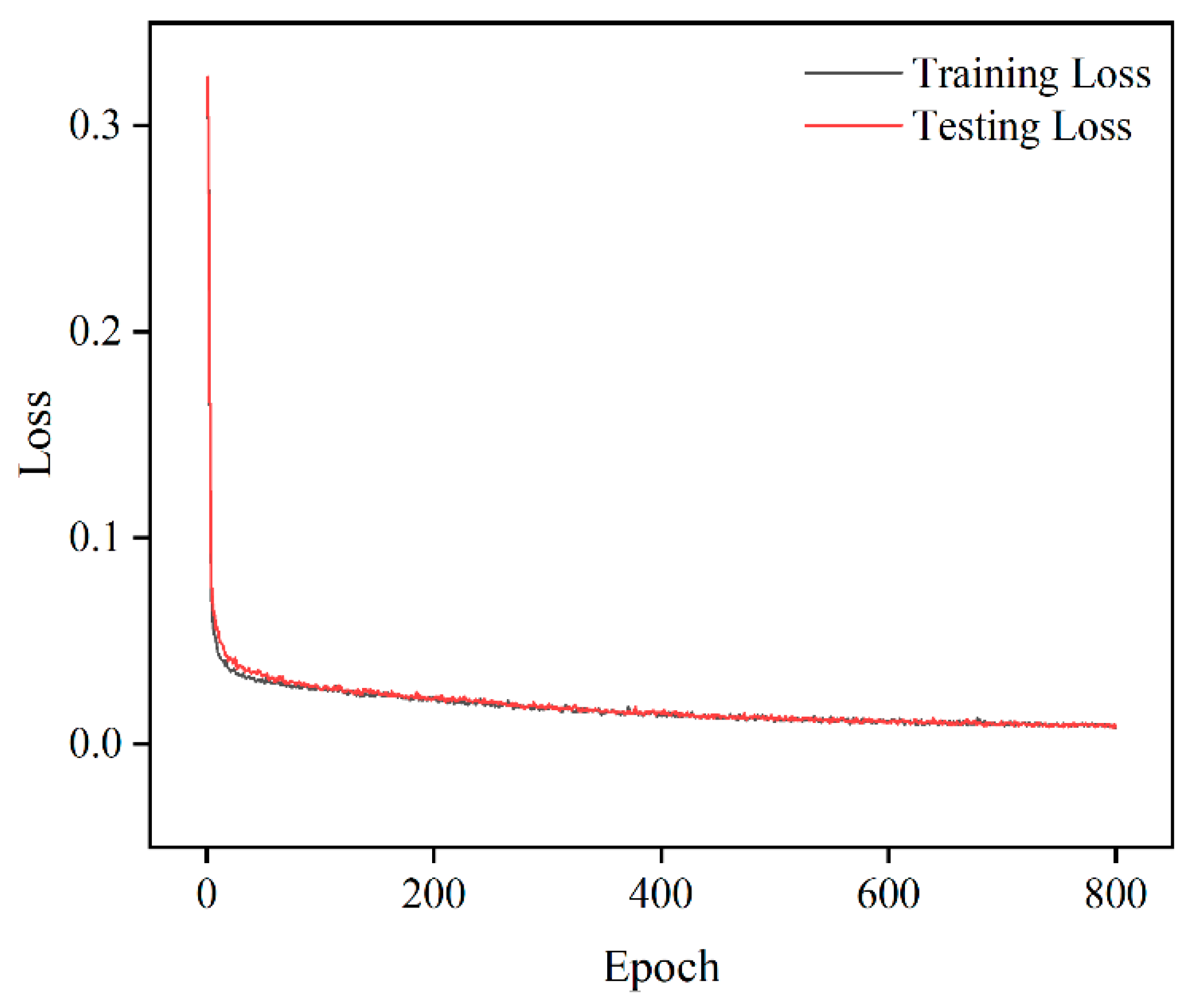
Based on the dimensionality-reduced dispersion features, a tandem neural network (TNN) is constructed for the inverse prediction of the material microstructure images (40 × 40) and three-dimensional parameters. The network includes 10 fully connected hidden layers, supports multi-branch output, and is trained using a combined Mean Squared Error (MSE) loss function. The loss function of the model during 800 iterative training sessions is shown in Figure 13. The training loss function and the test loss function in the figure show a convergent trend, indicating that the network has been effectively trained. The time required for the network to undergo 800 iterative training sessions is approximately 310 s, and the accuracy of the structural images on the validation set reaches 98.43%.

In order to verify the effectiveness and rationality of the improved autoencoder in the task of compressing high-dimensional dispersion curves, the effectiveness of three methods, namely, no dimensionality reduction, dimensionality reduction by K-means clustering, and dimensionality reduction by autoencoder, is compared in inverse networks, respectively. The comparison indicators mainly include prediction accuracy and training time, and the relevant results are shown in

Table 3. Comparison of dimensionality reduction methods (no reduction, autoencoder, K-means with epochs = 800, Batch_Size = 64).

Algorithm	Accuracy	Time (s)
Not	98.54%	358
K-means	97.37%	336
Autoencoder	98.43%	310

.

The experimental results show that, without dimensionality reduction, although the model can directly use the complete 186-dimension dispersion curve as input and can finally obtain a prediction accuracy of 98.54%, the training time is the longest, reaching 358 s. The K-means clustering method compresses the feature dimensionality, but due to its failure to efficiently capture the nonlinear feature structure in the data, it results in a decrease in the prediction accuracy to 97.37%, and the training time is 336 s, which fails to bring significant efficiency improvement. In contrast, the autoencoder method adopted in this paper effectively compresses the input feature dimensions while maintaining a relatively good reconstruction ability. Finally, the training time is reduced to 310 s with high accuracy (98.43%), which is a 13.5% reduction in training time.

The comprehensive comparison shows that the dimensionality reduction strategy based on the autoencoder proposed in this paper not only has a stronger representation ability but also demonstrates good accuracy and better training performance in practical prediction tasks.

5. Conclusions

This paper focuses on the problem of efficient structure–dispersion curve mapping for 2D acoustic metamaterials, and forward prediction and inverse design frameworks that integrates multiple deep learning mechanisms are constructed. A CNN network incorporating the CBAM attention mechanism and FPN (multi-scale feature extraction) structure is effectively trained to achieve highly accurate forward prediction from structural images and material parameters to 186-dimension frequency dispersion curves. The experimental results show that the model achieves 99.65% prediction accuracy on the test set and exhibits good fitting stability in multiple frequency bands.

In the inverse design part, the proposed improved autoencoder compresses the high-dimensional dispersion curves into a 36-dimension space, which effectively alleviates the dimensionality catastrophe problem. The combination with the TNN tandem network can accurately predict microstructure images and material parameters. Compared with no dimensionality reduction, the training time is reduced from 358 s to 310 s, which reduces the training time by about 13.5% and achieves a better balance between efficiency and accuracy. This method not only improves the efficiency of reverse design but also shortens the design cycle, providing a more efficient and accurate solution for metamaterial design.