Geometrical Similarities Between Metallic Real and Computationally Simulated Grain Structures (Equiaxed Polygonal Grains)

Abstract

Metallic materials are formed with grain structures which are naturally formed during solidification or modified after any manufacturing process, such as rolling, cutting, machining, welding, etc. Grains with different sizes and geometrical morphologies have a strong influence on the micro- and macro properties of metallic materials. This is the reason why many authors have worked on computer simulations based on numerical methods, applying chaos theory and using graphical techniques for its reproduction. Thus, this manuscript is focused on the comparison between grain structures obtained computationally with grains in real metallic samples. The analyzed structures in this work were polygonal and equiaxed, they resulted from a dynamic evolution in which nucleation and growth procedures were simulated. Then, computational algorithms and standardized procedures were used for characterization. Thus, in order to demonstrate the geometrical similarities and differences in mathematical terms, similarities between sample features were calculated, measuring sizes and populations along different directions which could be used to establish rules and parameters for the appropriate control of nucleation and growth. Furthermore, the influence of the computational methods for simulation and characterization are also described in detail.

1. Introduction

All metallic material is formed with a chaotic grain structure. Primary, secondary, or modified, grain structures are formed in metals during the solidification process or are modified during the manufacturing processes due to the heat transfer influence and re-crystallization; consequently, there are many different grain sizes and morphologies [1,2,3,4]. Some grains have a columnar or equiaxed morphology; however, others can be polygonal or have more complex geometrical features [1,2,3,4,5,6,7,8,9,10,11,12]. Thus, the computer simulation of grain structures is a complicated problem due to their heterogeneity and capricious morphology [1,2,3,4,9,13,14,15,16,17,18,19,20]. These geometrical forms cannot be represented using only Euclidean geometry, i.e., straight, parabolic, hyperbolic, or alternated lines, because these are always on the boundaries of grain structures without any apparent reason or established rule [5,6,7,8,11,12,13,14,15,16,17,18,21]. Thus, the appropriate methodologies for representation have been taken into account. Mathematical and computational tools such as chaos theory provide statistical information, while programming algorithms have been used as a theoretical background for analysis. Nevertheless, establishing rules and programming algorithms for appropriate representations is not an easy task [3,4,5,9,10,11,12,16,21]. Moreover, the dimensions of grains can be in the range of many nm² to a few μm² or mm²; as a consequence, equivalence with respect to scale must also be calculated [2,3,4,5,6,11,12,16,17,18,21,22,23,24,25,26,27,28]. Many authors have developed models based on random walk, probabilistic distributions, cellular automata, and the random formation of geometries, including the Monte Carlo method, obtaining realistic results for creating virtual grain structures [5,6,7,8,9,10,11,12,13,15,16,21]. Chaos theory allows the inclusion of statistical analysis, random number generation, and other unruled processes to represent any phenomenon [16,17,18,19,20,29,30,31,32,33]. Chaos theory has also allowed the development of different solving methods considering different assumptions when multi-variable situational cases are involved, finding different ways to solve these problems. In material sciences, different grain structures can be obtained as a function of different simulation methods and assumptions [6,7,8,9,10,11,12,15,16,20,21,34,35,36]. Recently, chaos theory has become a new exploration area and has been successfully used by many authors in many areas to solve problems such as the following:

• Unpredictable behavior in materials heterogeneity;
• Virtual earth geography and geology;
• Complex geometries in nature like flowers, branches, and feathers;
• Heterogeneous forms such as rocks;
• Fluid flow mixes;
• Cracks and failures in materials;
• Creation of virtual landscapes;
• Grain structures.

Many of these topics belong to different scientific areas, especially those related to microstructural analysis [1,2,3,4,5,11,12,16,17,18,19,20,21,22,23,24,25,32,33,37]. Starting with this, materials can be classified as crystalline and non-crystalline according with their atomic order. Grains in metallic materials are groups of thousands to millions of ordered atoms with a defined geometry, such as cubes, hexagonal prisms, octahedrons, etc. These materials present a repeated periodic order, necessary for the analysis of a poly-crystalline treatment [12,13,14,15,16,17,18,19,24,25,26,27,28,29,30,31,37,38,39].

In this work, to demonstrate the similarities and difference between real and simulated samples of grain structures, it was necessary to validate that all the samples contained polygonal equiaxed grain structure features; therefore, the following procedures were performed [9,10,11,12,16,17,18,21,27,28,29,30,31,32,33,35,36,38,39,40,41,42].

(1)

It was necessary to confirm that the grain structures in the computationally simulated samples were equiaxed. Then, the grain size along the horizontal and vertical axes needed to be counted to determine their similarity; the steps performed were the following:

(a)

Grain size was measured along the horizontal axis (counting the grain at every cell distance and averaging all values).

(b)

Grain size was measured along the vertical axis (counting the grain at every cell distance and averaging all values).

(c)

Both values were corrected as a function of their length and compared.

(2)

It was necessary to confirm that the grain structures in the real samples were also equiaxed. Then, the samples were prepared and scratched for testing; after that, the metallographies were photographed with an optical microscope and measured as follows:

(a)

Real samples were divided to be classified, taken as rectangular and square samples; this action was conducted to confirm that both sample regions had equiaxed grain morphology.

(b)

Both real samples were measured along the horizontal axis.

(c)

Both real samples were measured along the vertical axis.

(d)

Additionally, the samples were also measured as a function of a radial position, in order to verify again that all real samples had an equiaxed grain form.

Finally, the concepts for the simulated and real samples were compared with each other.

Some authors have made computer simulations of grain structures, mentioning their similarity with real samples. They have used a variety of different numerical methods according with the technologies and mathematical resources disposed. Initially, the problem was treated as an isolated phenomenon using models with a random formation using a random walk method, where short or long steps for the walker were taken as vertexes; then, defined lines were displayed to join them as grain boundaries [6,9,10,11,12,15]. The results were grain structures with an amorphous appearance [1,2,3,4,5,6,7,8,19,20,22,23,24,29,30,34,35,36,37]. This method was employed by beginners and enthusiasts in the 1970s and 1980s when computers had limited data management speed and storage [6,7,8,10,11,12,16,17,21,22,32,33,37]. The similarity with real grain structures was evident, but the display was extremely primitive and the models worked without a correlation with any physical phenomenon; nevertheless, many authors and enthusiasts continue using it to the present day due to its simplicity [9,13,14,15,17,18,19,20,22,23,24,25,26,34,35,36]. However, these computational models based on basic chaos theory can represent only a few features of the grains structures such as grain boundaries, vertexes with different coordination, and different grain sizes. Unfortunately, these methods have limitations in creating more complex grain structures. Consequently, it is difficult to simulate complex grains and other phenomena such as those formed by coalescence phenomena during nucleation and growth at different times [17,18,19,20,22,23,24,25,26,27,30,34,35,36,40,41,42,43,44]. This happens frequently when two different grains are grown along the same growing direction and are joined at any time during simulation, forming geometrically complex boundaries [1,2,3,4,5,6,7,8,19,20,22,23,29,30,32,33,34,35,36,37].

Models which simulate grain nucleation and growth allow us to appreciate grain formation as a function of the time, allowing consideration of more than one nucleation period if required; then, the influences of both processes can be appreciated [6,7,8,13,14,29,30,31,32,34,35,36]. Recently, other authors tryed to include factors such as machining, mechanic stress, or thermal behavior in the solving algorithms because it is known these processes when industrially applied modify the original grain structure formed during solidification [3,4,5,9,11,12,13,14,15,16,17,21]. Others have used fractals, statistical theory, random number generators, and cellular automaton methods for describing the phases and grain transformation with special interest in ferritic steels [9,10,11,12,15,16,18,19,20,21,29,30,31,34,35,36]. These authors have shown their satisfactory results in prestigious materials science and mathematical publications, observing similarities between their structures and real samples. However, specific rules, procedures, and methods to create a virtual specific grain structure must be validated to provide certainty and thus provide appropriated recommendations about how to simulate any specific grain morphology [2,3,4,5,6,7,8,9,13,14,15,29,30,31,32,33,36]. In consequence, validation using mathematical criterions and measurement methods is required. Furthermore, some authors have developed graphical tools to clean grain structures, eliminating possible computer errors and numerical inconsistences which provoke defects during simulation, obtaining an ideal structure ready to be analyzed [4,5,6,7,8,13,22,29,30,31,32,33,36,37]. Some geometrical situations which can generate problems on the drawing in the screen are the following:

(a)

Random grain size (large and small grains).

(b)

Random grain boundaries morphology (straight and hyperbolic boundaries).

(c)

Random grain mixed boundaries (sophisticated combined boundaries).

Others have developed sophisticated models to simulate grain growth and the influence of the remaining time in a mushy state on the grain orientation and grain morphology during the solidification of square billets, large slabs, or another ferritic and non-ferritic alloys [6,7,8,10,11,12,13,21,29,30,31,34,35,36]. Additionally, some of these authors established parameters to simulate the frontiers between chill, columnar, and equiaxed zones of steel billets during continuous casting, obtaining a successful relation between the thermal quenching of steel and controlling the heat removal conditions [1,2,3,4,10,11,12,21]. Nevertheless, this kind of simulation is highly complex because the thermal behavior must be solved to create a primary grain structure; the rules must be applicable and specified for simulating different heat removal conditions; and thereby, the problem is treated to be solved separately after solving the heat removal. Instead, these authors demonstrated that a dynamic simulation of the grain growth process was feasible and this fact considerably reduced the computational effort [4,5,6,7,8,9,10,11,12,13,16,19,20,21,34,35].

It must be commented that many authors have worked using different models, including deterministic and chaotic models, to find relations between mathematical problems to reproduce processes and geometrical forms in nature. Beginners have used their limited computational capacities to perform this, but material scientists and metallurgists have still been working on improving these and developing new ones, and they have obtained very realistic structures; nevertheless, the problem of finding effective and suitable controls of mathematical parameters for simulating any kind of structure remains [1,2,3,4,8,13,14,15,16,17,18,19,20,34]. Furthermore, some authors have been studying the grain features, establishing relations with micro- and macromaterials’ properties [6,7,8,9,13,14,15,20,29,34,35,36,39,40,41,42,43]. This began with the relation between grain formation from liquid melting metals during solidification [1,2,3,4,5,17,18,19,20,34,35,45,46,47,48,49,50]. Some of them have worked in metallization, promoting the formation of a specific phase [22,23,24,25,26,40,41,42,43,44]. Others have demonstrated the evolution of microstructure as a function of other manufacturing processes or heat treatments applied which involve re-crystallization events [16,17,18,19,20,30,34,35,42,45,46,47,51].

Thus, one of the purposes of this work is to contribute to understanding the influence of the mathematical parameters that rule nucleation and growth in order to forecast a probable grain structure morphology and size. Furthermore, we aim to provide feasible geometrical parameters to establish similarities and differences which can be used to relate the principle with different other metallic materials [14,15,16,17,18,19,20,21,32,33,34,35,36,42,47,48,49,50,51].

2. Atomic Theory for Explaining Grain Structure Formation

Atomic theory is very important for understanding grain structure formation. Grains are present in metallic materials and form geometrical structures such as cubes, pyramids, and prismatic arrays like hexagonal arrays; these ordered formats are known as crystals. These materials can be classified as crystalline or non-crystalline solids. 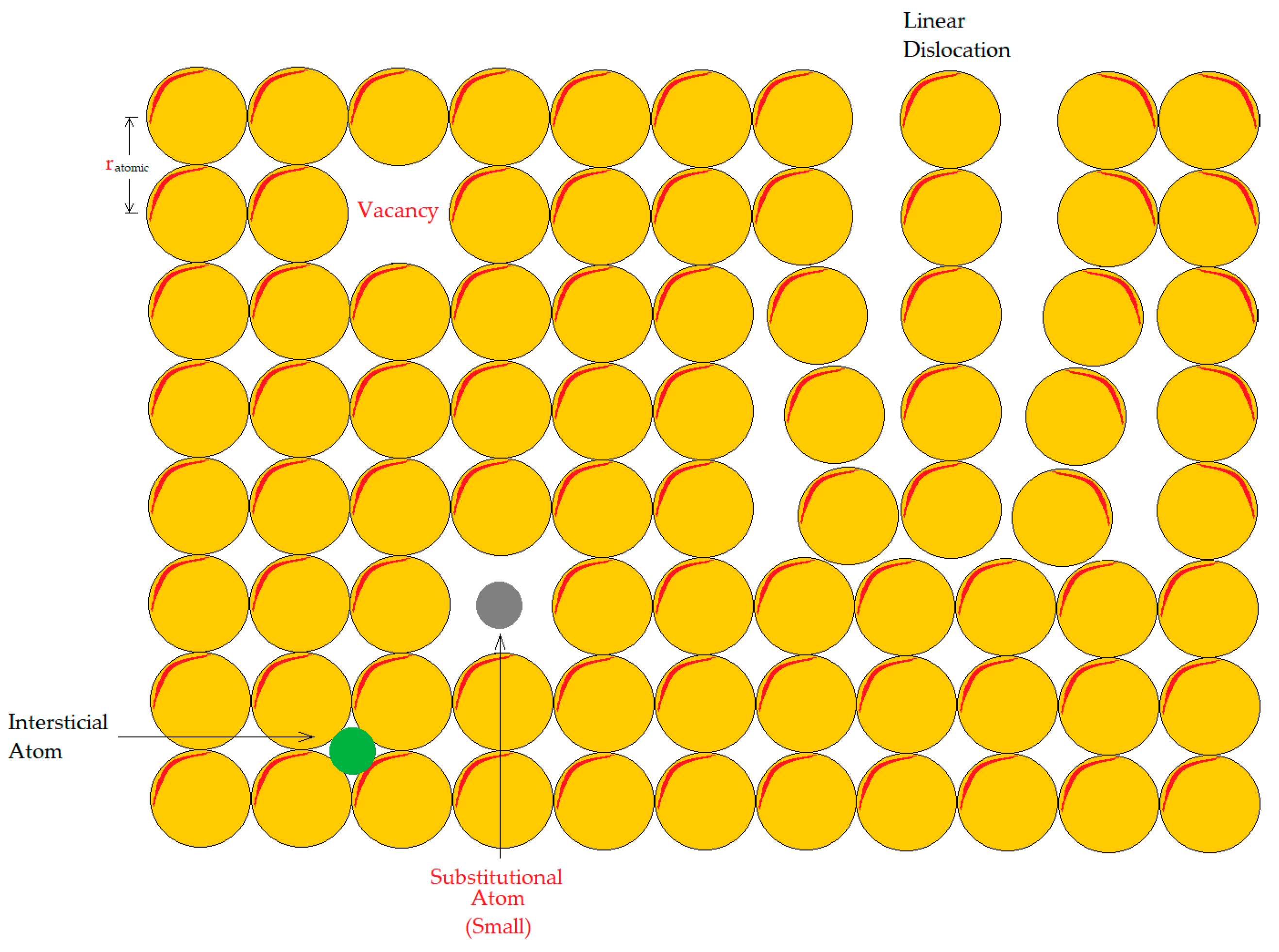Here, some parameters in the elementary atomic order in crystals can be measured in angstroms 1 × 10⁻¹⁰ or pico-meters 1 × 10⁻¹². The atomic radius increases in the periodic table from up to down and from left to right according with the number of protons, nucleons, and electrons; Dalton’s atomic model with spheres is a typical geometrical format for representing metallic groups. Then, a perfectly ordered crystal can be represented exclusively with atoms of the same element, or a group of a pair of atoms of the same elements always in the same periodic order as in a NaCl crystal. The atomic radius and cell parameters of structures are measured from nucleus to nucleus on the atomic periodic order as shown in Figure 1. Here, an imperfect crystal is shown, due to its many localized and linear defects.

Metallic structures are formed with thousands and millions of these atoms originally in melting; then, these atoms with energy loss mobility during solidification and form consolidate groups. It is complicated to separate them exclusively to have only atoms from a simple common element. Then, atoms of other elements frequently are found between the atomic lattices forming defects. Some frequent defects in an ordered structure are also shown in Figure 1. Here, a 2D array of atoms ordered is shown and defects such as vacancies (unfilled spaces between the atoms), substitutional atoms (atoms of others elements occupying a place on the metal lattice), and interstitial atoms (atoms in unfilled spaces between each other) can be appreciated. These are considered as defects because their presence alters the original order of a perfect crystal; additionally, these are also known as local defects or 1D defects. Nevertheless, according with analysis, there are 2D and 3D defects—these kind of defects are dislocations and affect the order of atomic groups as shown in the same Figure 1, generating stress. In addition, there are defects that co-exist in pairs and are related with the electronic disposal of the cations and anions in the crystals such as Frenkel and Schottky defects. Furthermore, inclusions are another kind of defect considered as undesirable elements in the metallic material or alloy which often affect the material properties, becoming dangerous corrosion sites or weak regions. It is highly important to understand these topics, due to these representing the basic knowledge needed to support materials science technical theory.

It is important to mention that the computer algorithm developed by one of the authors can be used to reproduce the atomic order when a group of atoms form a grain, but the appropriate assumptions must be taken into account, such as the following:

(a)

One cell is an atomic single site; thus, one cell represents one atom.

(b)

As the scale for simulation is so small, only a few grains must be defined as nucleated points.

(c)

The growth process will be executed many times in order to fulfill the unsolidified zones.

The result is a very fine forming of grain boundaries. The samples are equivalent at a very small scale: 1 × 10⁻¹⁰. Moreover, it is possible to simulate vacancies, declaring empty spaces randomly distributed inside the simulated sample, while substitutional atoms and atoms of inclusive elements can also be included in the simulation taken as a minimal percentage of them and indicating a random appearance of these.

There are cases when a longer dimension is simulated, like measurements in microns 1 × 10⁻⁶ m. Herein, every cell represents a group of a hundred atoms which form the grain boundaries at a very large scale size in the simulation. Here, inclusions can also be included in simulations, as well as declaring portions of other undesirable elements. Moreover, empty zones can be declared to simulate blowing and incomplete fulfillment problems. But, these options are far away from the purpose of this manuscript, although the present authors are preparing work to address these topics.

According with the grain sizes in microns; in the present work, the tool used for the analysis of the real samples was optical microscopy; although, assessment of the grain boundaries’ morphology required preparation and scratching for characterization via observation and measurement.

Heat transfer is a very important knowledge area for metallurgist and material science. Heat transfer is related with solidification, but also with heat treatment, re-crystallization, and phase transformation. Some of the present authors have worked on the heat removal process during solidification and solving equations for conduction, forced convection, and radiation, and their experiences provided physical limits for understanding grain morphology as a function of the solidification speed in steel billets produced by continuous casting during ironmaking and steelmaking industrial processes [6,7,8,11,12,16,17,21]; we recognize that the relation between both phenomena is highly important.

3. Equiaxed Grain Structures with a Homogeneous Grain Size

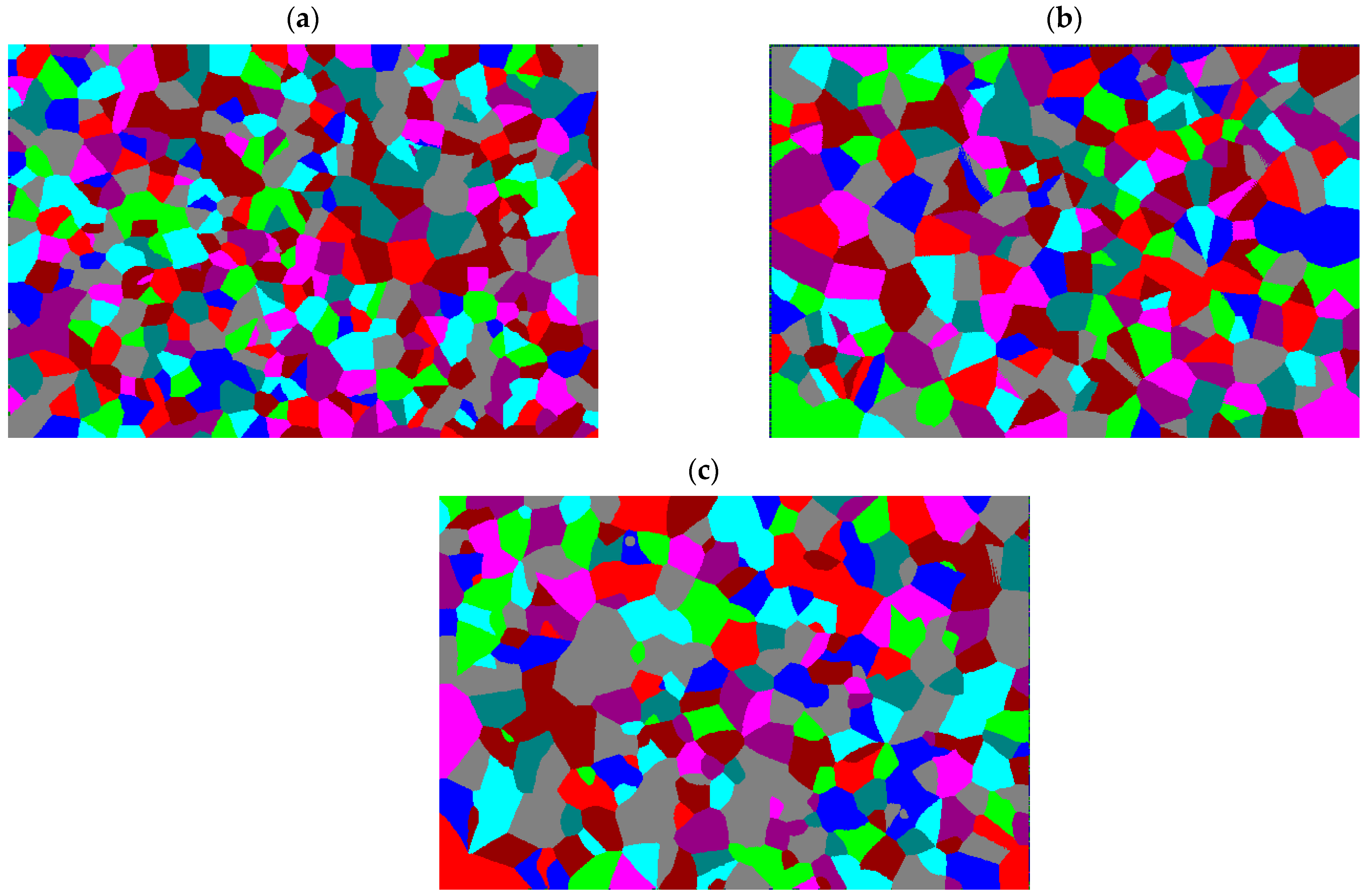
Figure 2a–c show the computationally simulated grain structures which were analyzed in this work; these are equiaxed and polygonal grains with small, medium, and large sizes within them [29,30,31,32,36,40,41,42,43,44,51]. Moreover, it is possible to observe a homogeneous grain size distribution all around the grain structures without any preferential location. Here, many simple polygonal grains with a few complexes can be observed. Therefore, it is possible to affirm that these three structures look very similar. The grain structures were simulated using the algorithms previously described [43], in which the grains were formed by reproducing the nucleation and growth processes according with the parameters listed below [6,7,8,9,10,11,12,16,21,30,40,41,42,43,44,51].

(a)

Number of nucleated points at every nucleation period. This is the number of new nucleation points that will appear when the nucleation subroutine is executed. Moreover, every new point will potentially be a new grain and an ID color is assigned to each one. For the simulations in Figure 2a–c, we defined values of 210, 200, and 190, respectively, and this selection was conducted considering minimal grain size variation.

(b)

Number of nucleation periods. The influence of nucleation periods is appreciated in grain structures because points nucleated in the second, third, and next sequences are normally much smaller than those nucleated before due to there being fewer available surrounding neighbors for growth. For the samples simulated in Figure 2a–c, only a single period was declared in this work. Consequently, variations in the grain size populations are almost unappreciated.

(c)

Iterations executed before a new nucleation. This is an integer data type and is the number of growth subroutines executed before a new nucleation subroutine is executed again. For the samples simulated in Figure 2a–c, 30 steps were defined. This number is considered high enough to complete the growth process with any remaining unavailable cells.

(d)

Growth direction of the nucleated points = all around, 360°. It is defined as the angle of growth of every nucleated point, where 360° means that the nucleated point can grow all around at least any other point which occupied the nodal position before. In other words, the cell was not available and belonged to other grain.

(e)

Growth radius for every iteration = 1. This value controls the growth subroutine and forms the perimetral limit of the grain. This value is highly important because it represents the speed of the advanced front surrounding every nucleated point.

Different simulated grain structures were obtained as shown in Figure 2a–c. The sample in Figure 2a shows a grain size that is almost homogeneous along the horizontal and vertical axes. In the sample in Figure 2b, there are a few small grain neighbors surrounding grains with a regular average size. In the grain structure shown in Figure 2c, there are large grains with others being very small. Thus, these three grain structures have similar features but also clear differences. But, for an appropriate comparison, these structures must be measured to be described mathematically and geometrically.

The simulated samples in Figure 2a–c were obtained dynamically—this means as a function of a nucleation and growth procedure, not using a simple random location of vertexes as was performed at the beginning of the materials science crystal-forming simulations. This fact can be noticed because these samples have straight but also hyperbolic grain boundaries; in addition, the formation of complex grains can also be appreciated, as the only way to obtain these structures with a random walker model is by modifying the original algorithm and including sub-divisions between the previously defined grain coordinates. Moreover, the identification of different colors forming grain boundaries also evidences the structures resulting from a dynamic process.

Every grain structure in Figure 2a–c is different; here, every color represents a specific grain, but the color does not represent any specific phase. Normally in metallic material, there are only a few grains; for example, in low-carbon steel, only perlite and ferrite are represented in a typical grain structure [6,7,8,11,12,21,40,41,42,43,44]. Nevertheless, a researcher can assign a value for any phase, transforming the original sample in a bi-color format. The grain structures in these figures were characterized, measuring their grain populations and sizes to compare them with the real sample features.

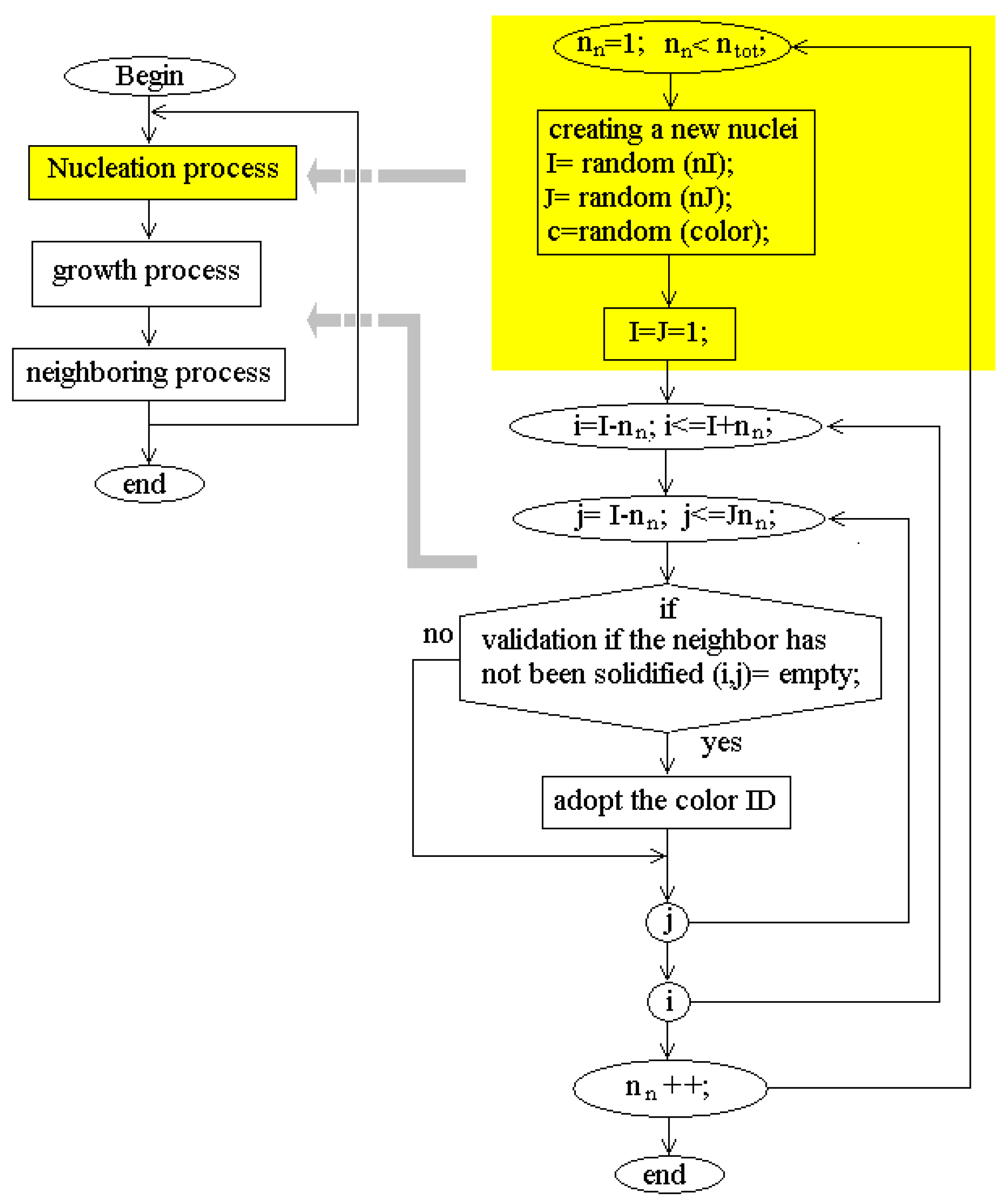
A description of how the nucleation and growth processes were taken into account and included in the simulation can be appreciated in Figure 3. Here, simulated samples were obtained considering only a single period of nucleation; therefore, the nucleation routine in the shaded zone is executed a single time but is used to create all the nucleated points; then, the growing routine is executed many times until there are no available neighbors; the neighboring process is very important in order to find the nearest points to the solidified points and make these adopt their colors to form all solidification fronts of every grain. In this flowchart, the variables (I) and (J) are used to indicate every nodal location, and the variables (i) and (j) are used to indicate the nearest neighbors to the nodal points. A nodal point is the analysis point under analysis to find every new available node. Additionally, in this flowchart, where the values from I = J = 1, this means that the point is placed in the upper-left corner of the simulated sample; consequently, if I = nI and J = nJ, this means that the point is in the lower-right corner position. Here, the increment is conducted one by one, step by step during grain formation.

An additional simulated case, shown in Figure 4, this, represents a dynamic simulation of a grain growth sized as nI = 600 and nJ = 400, with the following features:

Nucleation periods: 2.

Number of nucleated points in every nucleation period: 300 in the first and 150 in the second.

Steps for growth between every nucleation period: 20 and 10, respectively.

In Figure 4a–c, the evolution of grain structure formation is shown. In Figure 4a, the nucleation process begins to execute the routine to produce all the randomly nucleated points. In Figure 4b, the growth procedure has been executed many times, and it is possible to appreciate that some grains have growth until being blocked by the growth of other nucleated points growing simultaneously. Moreover, it is possible to see that some grain boundaries have formed; there are some unsolidified zones and other grains continue growing. In Figure 4c, the simulation has finished and the resulting grain structure is shown entirely.

4. Algorithms for Characterization of Simulated Samples

Then, in this work, a set of computationally simulated 2D grain structures are compared with real samples taken from metallographic optical microscopy; both kinds of samples have polygonal equiaxed morphologies [9,10,11,12,16,17,18,21,22,23,26,27,28,31,32,33,37,38,39,40,41,42,43,44]. Characterization methods for grain size provide accurate information about the grain morphology. Computational tools can provide more detailed data about geometrical features such as the grain population, grain distribution, grain size along the horizontal and vertical axes, and grain area of the simulated samples [22,23,30,31,32,33,37,40,42,43,44,51]. The simulated grain structures are images formed with pixels displayed on the computer screen; the samples are square or rectangular regions with different grain populations; regular square meshes are used for discretization; and the sub-indexes (I) and (J) are used to indicate every cell position [9,10,11,12,16,21,28,38,39,40,41,42,43,44]. Here, the equivalent ratio is that 1 cell is 1 pixel color, and a palette with a numerical code is defined for identification. A 2D computational array of integer variables is named to store the information [3,4,5,6,7,41,42,43].

To evidence a correspondence between the real and simulated samples, a relation between the number of cells used to simulate a grain structure with the real dimensions of a metallic sample using optical microscopy must be established as shown in Equation (1). Here, nI and nJ are the number of cells used to computationally simulate the grain structure along the horizontal and vertical axes, respectively, while lx and ly are the real sample dimensions. In an analyzed grain structure, grains can have very different sizes and morphologies.

Typically, a grain structure is treated as a population of grains in a captured region. Consequently, grain size can be expressed measuring every grain’s area as a function of the total area of the sample; the resulting values will be parameters that will allow geometrical measurement for comparison.

As can be appreciated, the same notation is also used for the simulation and characterization of the simulated samples, and Equation (1) can be used to express the relation between the real and simulated grain structures.

$${\displaystyle \frac{nI}{lx}}={\displaystyle \frac{nJ}{ly}}$$

(1)

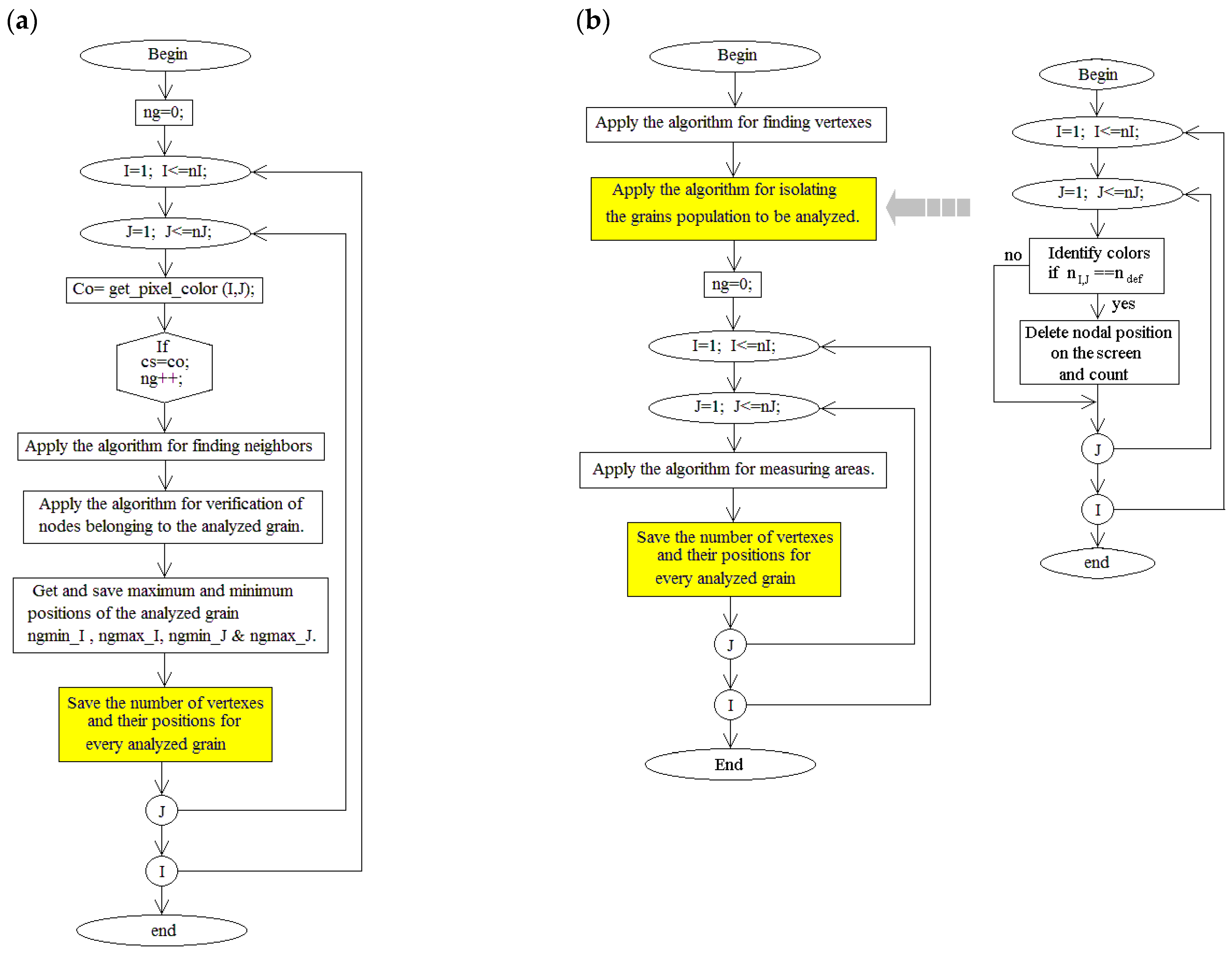
Figure 5a,b show the procedures for the characterization of grain structures. The routines employed in this research for measuring areas and finding vertexes were detailed in a previous work [38,39,40,41,42]. These two algorithms can be used for an entire characterization; although as can be seen in these flowcharts, the order of the subroutines’ execution can be modified according with the geometrical features to be measured, and the results are counted and classified automatically, showing the information conveniently grouped. In these flowcharts, the variable co takes the value directly from the color on the screen of the cell in the position (I, J), which is compared with the color (cs) of the original grain taken; then, a neighboring process is executed to know whether there are any other neighbors with the same color; this process is executed until there are no neighbors, verifying this condition; and then it is considered that all the nodes of any specific grain have been found and validated. ng is a counter for every grain with the color selected to be measured; therefore, it must initialized as equal to zero at every execution of the routine.

The algorithm in the flowchart of Figure 5b shows an alternative way of performing the same analysis; here, the algorithm for finding vertexes is executed first and independently. Then, the population of grains to be characterized is separated from the original grain structure and the screen is cleaned; then, the next pair of loops are executed to analyze the sample, measuring the grain areas and the increment of the variable ng is nested in the analysis subroutine which means the counting of every new grain [23,24,25,26,27,28,30,40,41,42,43,44,45,46,47,51]. The procedures in the flowcharts are well known as filters and perform specific processes to characterize the samples; therefore, these are very important to show the original grain structure borders and vertexes. Moreover, computer-programmed filters help to identify a particular feature of the grain structure and allow us to measure and classify every grain [24,25,26,27,28,30,38,39,40,42,43,44]. The increment in every loop of both flowcharts is performed one by one, step by step during characterization.

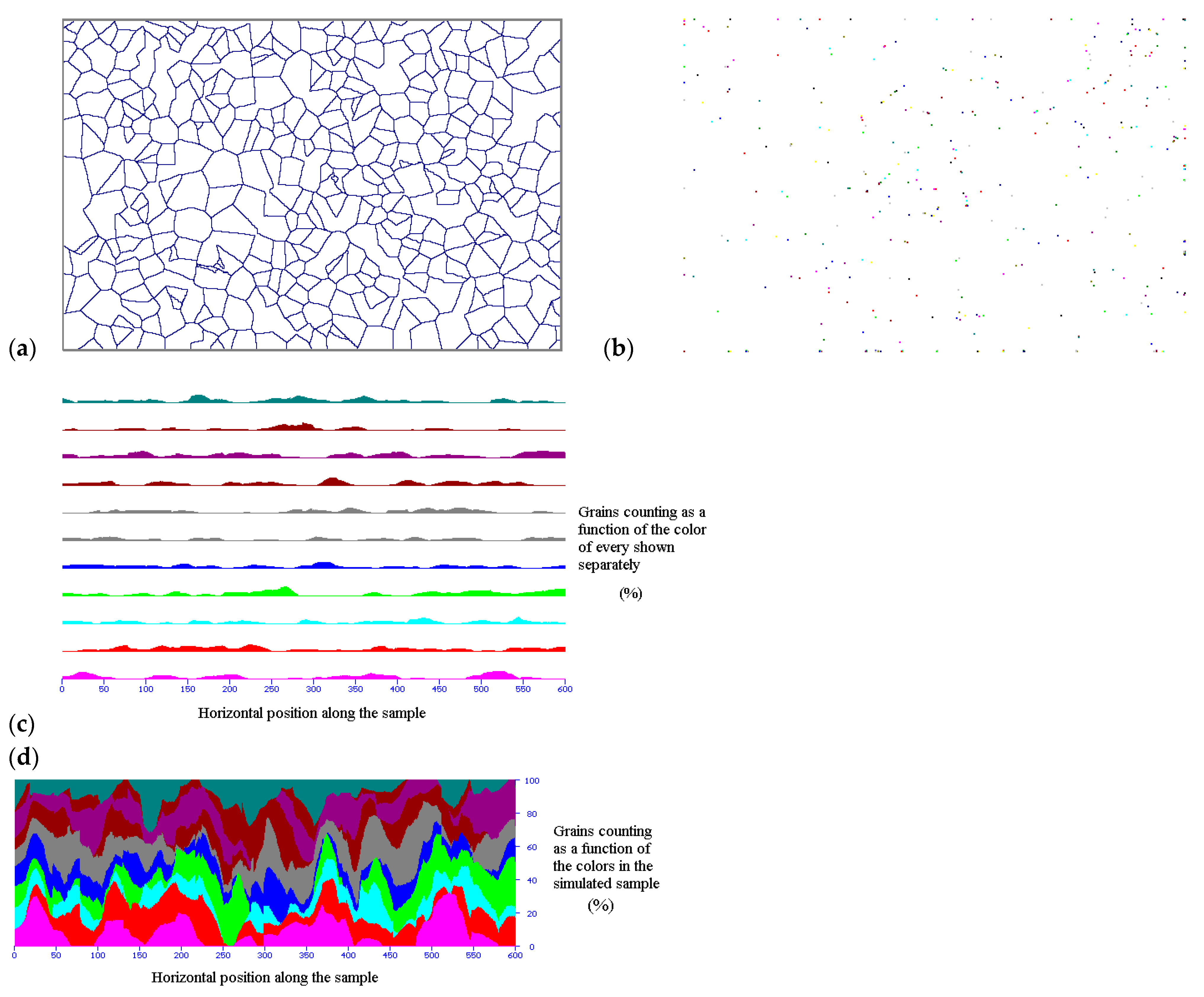
The procedure for the characterization of the computationally simulated samples can be appreciated in Figure 6a–f, which show some actions the filters can execute to characterize the sample described in the flowcharts before. Figure 6a shows the application of a computational filter capable of recognizing grain boundaries and marking them. The result is a characterized grain structure similar to that obtained after the application of light scratching in a real sample [30,40,41,42,43]. The application of this filter cleans the grain structure, allowing us to appreciate the grain boundaries. Then, a binary 2D computational array is used to save the information.

Figure 6b shows the execution of a computational filter capable of finding all the vertexes in a simulated structure. Here, the intersection of more than two borders in a common point is identified and marked. The resulting information can be stored in a separated file for easy management. The values stored are the coordinates (I, J) of every vertex using an integer data type in an ordered format.

Figure 6c shows the grains counted along the horizontal axis. As can be appreciated here, there is a similar behavior and similar fluctuations in colors; moreover, the total average of the grain count is also similar. Figure 6d shows the local distribution of the grain population in a cumulative graph. These figures both show the classification of the grains as a function of the colors for every horizontal position in a separate and cumulative format; these graphs allow us to identify the grain presence as a function of the colors defined. In contrast, Figure 6e shows the grain size population distribution as a function of the measurement of every grain area.

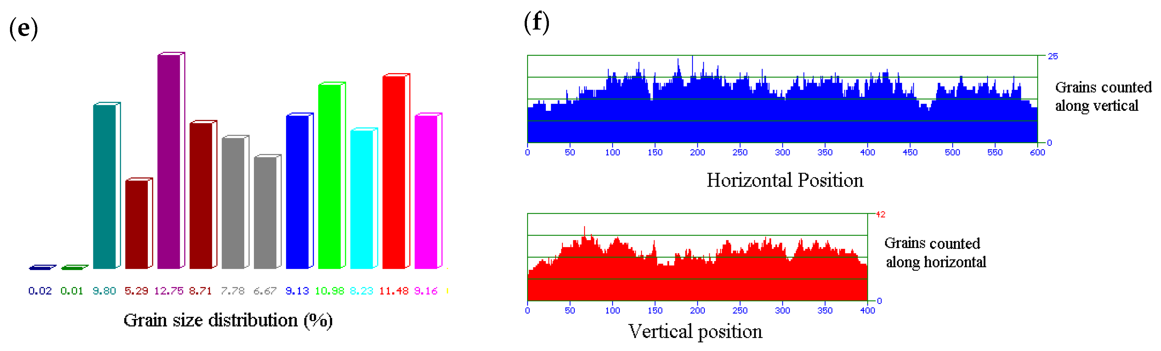
Figure 6e shows the counting and classification of the grains as a function of the grain size. As almost all of the values presented seem to be very similar, it is possible to affirm that there is a homogeneous distribution of different grain sizes along the sample. Additionally, the difference between the sizes is not very significant, evidencing that grain size also tends to be homogeneous or shows a minor difference.

Figure 6f shows a pair of histogram curves. Here, the grain populations along the horizontal and vertical axes were counted—the scales are different, but the following procedure was taken into account to evidence that the grain size is very similar along both axes. Every process in the computational characterization is conducted automatically, the results can be expressed in graphical formats, and finally calculating continues, resulting in a single numerical averaged value.

The simulated grain structure dimensions in this work were nI = 600 and nJ = 400. The results after characterization for the three samples are shown in

Table 1. Average values for the grains counted in the computationally simulated samples.

Sample	1	2	3	4	5	Average
Horizontal	20.251	20.452	20.512	20.442	20.364	20.405
vertical	30.768	30.663	30.546	30.376	30.678	30.604

; these values were averaged and divided between their longitude in pixels, obtaining similar values, finding that the grain size is almost identical along both vertical and horizontal axes, evidencing equiaxility.

Equations (2) and (3) were solved for the horizontal and vertical axes, finding very similar values; consequently, the grain was verified as equiaxed. Here, the fraction 400/600 is a correction applied due to the dimension of the rectangular sample. Now, multiplying the grains counted for both axes results in the total grains in the simulated sample. Then, the total grains and average area of every grain can be calculated by solving Equations (4) and (5), respectively.

Figure 6f shows the histograms for both the horizontal and vertical axes. The values shown in Table 1 resulted from this count. Nevertheless, they are very different. Thus, Equations (2) and (3) are used to correct the grain count, considering the length of them as a function of the sample dimensions; then, the resulting values are very similar, evidencing that the grain size along both axes is also similar; thus, it is possible to affirm that the morphology of the grain structures are equiaxed.

$$A{g}_{ I}={\displaystyle \frac{{gs}_I}{nI}}={\displaystyle \frac{20.405}{600}}=0.034$$

(2)

$${Ag}_J={\displaystyle \frac{{gs}_J}{nJ}}={\displaystyle \frac{30.604\left(\frac{400}{600}\right)\left(\frac{400}{600}\right)}{400}}={\displaystyle \frac{13.602}{400}}=0.034$$

(3)

g_sizeI × g_sizeJ = 20.405 × 20.374 = 415.732

(4)

Here, Ag is the area for every grain and gs is the grain size average, taken from Table 1 along the corresponding axis. But, if the inverted operation is performed for Equations (2) and (3), the results are 29.412 and 29.507, which are again very similar and represent the average value in pixels for a grain. Multiplying these values, the result is 867.210 pixels, which is calculated using Equation (5); this is the average grain area in pixels inside the simulated sample.

$${A }_{grain}={\displaystyle \frac{n_I\times n_J}{{ng}_I\times {ng}_J}}={\displaystyle \frac{600\times 400}{20.5\times 13.5}}=867.210 \mathrm{p}\mathrm{i}\mathrm{x}\mathrm{e}\mathrm{l}\mathrm{s}$$

(5)

5. Analysis of Real Samples

Real copper samples were cut using a metallographic cutter machine and rough-sanded using different sandpapers; then, they were polished with alumina dust at 0.3 μm as a standard procedure recommended for preparation; and chemicals were prepared in the laboratory for scratching: the mixing relation was 3:1 of HCl/HNO₃. The standard procedure for average grain size measurement is well established by the ASTM [42]. This procedure was applied to count grains along the horizontal and vertical axes, identifying the borders; the results are shown in

Table 2. Grain size characterization along the horizontal and vertical axes for the real samples (counting of grains).

Sample	1		2		3		4		5
Measurement Position	→	↓	→	↓	→	↓	→	↓	→	↓
0	11	10	10	11	7	10	7	9	12	9
1.5	12	8	13	10	10	7	10	8	15	9
3	12	6	11	9	12	7	11	7	15	7
4.5	11	7	12	9	11	7	9	8	11	11
6	12	10	12	10	10	7	10	9	10	8
7.5	10	10	12	7	9	7	8	7	10	8
9	13	9	13	8	11	10	10	11	12	7
10.5	12	10	10	9	11	9	10	10	10	10
12	10	9	11	8	11	10	11	7	11	10
13.5	12	10	12	8	12	6	13	9	10	9
15	8	11	13	9	12	9	11	7	11	11
16.5	9	9	12	9	12	8	11	7	12	8
18	10	8	12	10	9	10	10	9	12	8
19.5		11		8		7		6		7
21		8		10		8		8		7
22.5		7		10		8		8		9
24		8		10		7		9		6
25.5		7		8		7		8		7
27		6		8		7		10		7
Sum	142	164	153	171	137	151	131	157	151	158
Average →	10.923		11.769		10.538		10.077		11.615
Average ↓		8.632		9		7.948		8.263		8.316
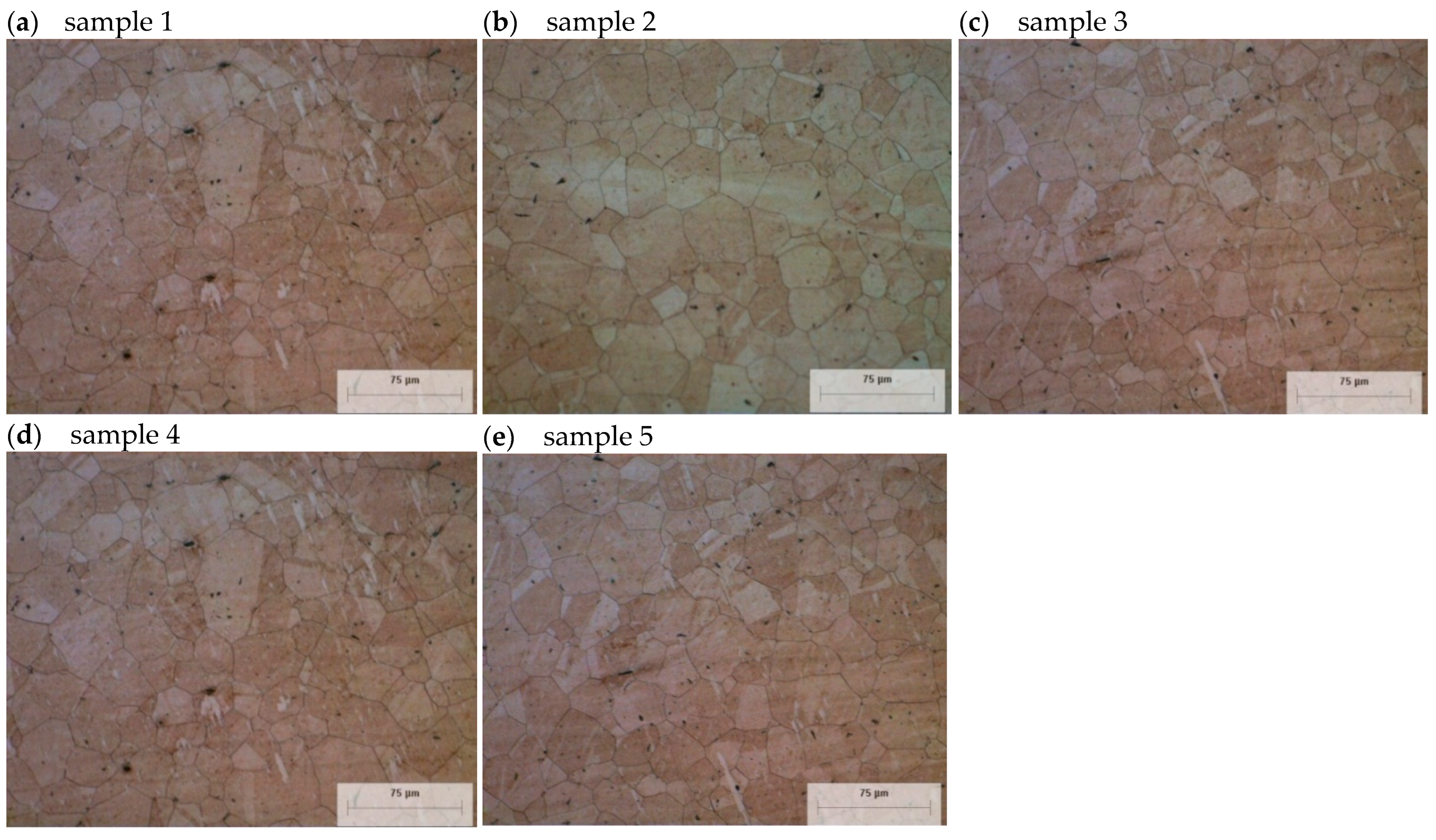
correction	8.767		9.446		8.458		8.088		9.323

. The real grain structures in Figure 7a–e were characterized. Here, different metallic samples were selected. In these figures, it is possible to appreciate polygonal and complexes of grains distributed all around; moreover, the grain size and morphology also seem to be similar but with particular details. Samples are considered according with their order in these figures. The grain structures in Figure 7a–e were captured using an optical microscope Instruments Nikon MA-200 Japan co with a polarized light to enhance contrast; these are very similar, and here it can be appreciated that all of them are equiaxed and with a polygonal form in every metallography. Moreover, different grain sizes can be found, some of them very large and others very small; the grain boundaries can also be easily identified. These figures were shaped in an optical metallographic microscope with a 50x lens.

The sum of the total horizontal grains counted vertically (↓) is 42.158. The average of the horizontal grains (↓) is 8.432. The sum of the total vertical grains counting horizontally (→) is 44.083. The average of the vertical grains (→) is 8.817.

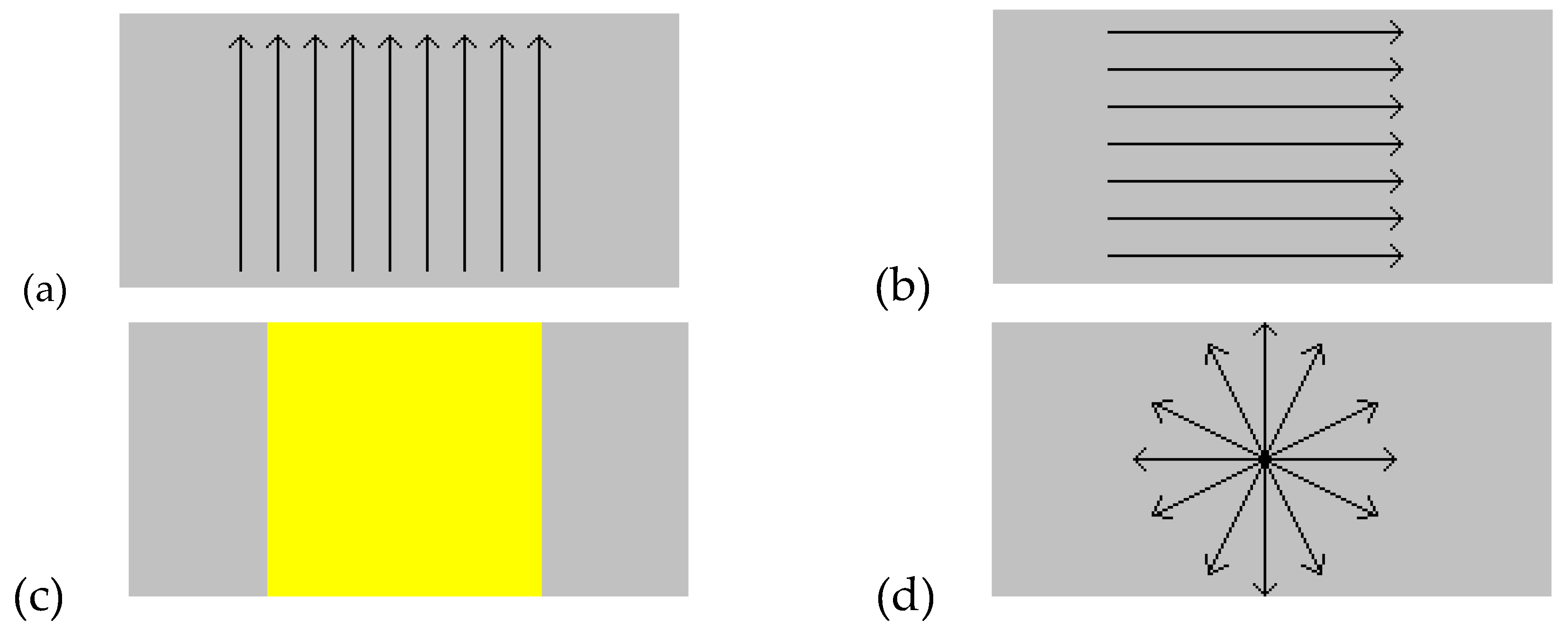
During this work, to ensure that the grains were truly equiaxed, similar values and dimensions had to be validated along different directions. Thus, in Table 2 the arrow → indicates that the grains were counted horizontally; then, these values were averaged to represent the entire grain number along the perpendicular direction (vertical). In this way, the arrow ↓ indicates that grains were counted vertically, in congruence with the directions for counting shown in Figure 8a,b.

A complementary analysis was conducted for the real samples in rectangular metallography (entire image) and considering a square area (from the same captured samples); additionally, another analysis along the radial direction was conducted to corroborate the presence of equiaxed morphology as a function of the measurement direction as shown in Figure 8c,d. Additionally, Table 2 shows the measurement along the horizontal and vertical axes of the grains for every real sample. Here, the values are added and averaged in the last two rows; these values are very different for both axes, but these are corrected as a function of the aspect ratio of the sample and averaged again.

Measurements were taken at the position indicated in the first column from left to right for vertical measures and from high to low for horizontal measures. The row of the sum represents the total grains counted in every sample. The measurement direction is indicated perpendicularly. As the metallography is rectangular, there are more horizontal measures than vertical. In consequence, there are more rows with values for the horizontal direction, in the same way as for the measurements of the simulated samples. There are average values along the measurement directions → and ↓. Here again, these values are very different because the measurements were made along the vertical axis. Thus, these values must also be averaged, dividing by the number of counts performed as indicated in the last row; then, these values were very similar in comparison with the average for ↓, evidencing that the grain sizes along both analyzed axes were very similar and the grain morphology was also equiaxed.

In the lowest rows of Table 2, there are values with the application of an aspect ratio resulting from the sample size (lx/ly) = (311.54/236.54) = 1.317. The resulting values are now much more similar, and the final averaged values are 8.432 for the horizontal axis and 8.817 for the vertical. Consequently, it is possible affirm that the grains in the samples are very similar along the horizontal and vertical axes; thus, the grain structures are equiaxed. Grain size is also similarly measured along the two axes. The total counting and averages are obtained by solving Equation (6) for both the horizontal and vertical axes. This procedure was conducted to calculate an average value and validate all the samples also presenting equiaxed morphology.

$$ng={\displaystyle \frac{\sum _{n=1}^{n=total samples}grains}{total samples}}$$

(6)

In order to compare measurements between rectangular and square samples, the total grains in both were calculated by solving Equation (7).

Ng_total = ng_{I average} × ng_{J average}

(7)

The values used and the results obtained are as follows.

Rectangular sample: 11.1044 × 8.817 = 97.902 grains.

Square samples were analyzed taking only the values in Table 2 into account; these are counted on both axes.

Square sample: 8.432 × 8.817 = 74.337 grains.

Assuming that for a square sample the dimensions along the horizontal and vertical axes are the same, then lx = ly, and for rectangular samples lx > ly. Then, the area average of the grain samples can be calculated.

The averaged grain area was calculated for a rectangular sample as follows.

Area of the rectangular sample: (311.541 × 236.540) = 73,691.672 μm².

$${A_{grain}{\displaystyle \frac{A_{sample}}{grains}}}_{total}={\displaystyle \frac{\mathrm{73,691.672}}{97.9025}}=752.705 {\mathsf{\mu }\mathrm{m}}^2/\mathrm{g}\mathrm{r}\mathrm{a}\mathrm{i}\mathrm{n}$$

(8)

Solving the same equation for a square sample, the same procedure was applied.

Area of the sample square: (236.54 × 236.54) = 55,951.1716 μm².

$${A_{grain}={\displaystyle \frac{A_{sample}}{grains}}}_{total}={\displaystyle \frac{\mathrm{55,951.172}}{74.3372}}=752.736 {\mathsf{\mu }\mathrm{m}}^2/\mathrm{g}\mathrm{r}\mathrm{a}\mathrm{i}\mathrm{n}$$

(9)

As expected, both values are very similar: 752.7047 and 752.736; therefore, considering a rectangular or square sample, the same average grain area appears in all of the samples. Thus, it is possible to affirm that the square and rectangular samples have a very similar grain size along the vertical and horizontal axes. Here again, the relation in Equation (10) can be solved to confirm the equiaxility, and the results are shown in

Table 3. Relation for the grains counted along the horizontal and vertical axes to evidence equiaxiality.

Sample	1	2	3	4	5
ngI/ngJ	1.016	1.049	1.064	0.979	1.121

, where all these values are near to 1. Then, all of the samples tend to be equiaxed; the biggest difference is in sample 6e, in which the grains tend to be slightly larger along the horizontal axis.

$${\displaystyle \frac{{ng}_I}{{ng}_J}}={\displaystyle \frac{8.767}{8.632}};{\displaystyle \frac{9.446}{9.000}};{\displaystyle \frac{8.458}{7.947}};{\displaystyle \frac{8.088}{8.263}};{\displaystyle \frac{9.323}{8.316}}$$

(10)

Statistical counts were performed automatically using the computational tools for characterization, as shown in Figure 6d–f which shows the grain populations and counting process resulting in the final numbers. In the same way, the characterization of physical samples in Figure 7a–e was conducted according with the ASTM procedures and then compared.

The grains were counted radially as a function of an angled position, and the calculation is described in

Table 4. Radial grain counting population on real samples.

Angular Position	Real Sample
	1	2	3	4	5
0	7	9	6	8	10
15	8	9	11	5	7
30	10	9	10	5	9
45	12	6	10	7	8
60	8	7	9	8	6
75	8	8	9	7	6
90	9	9	8	7	9
105	8	9	8	9	9
120	11	9	7	8	6
135	8	8	8	8	8
150	8	8	10	8	11
165	9	8	6	7	8
Sum	107	101	105	91	102
average	8.917	8.417	8.750	7.583	8.500

for the five real samples. Then, measurements were performed as a function of the angular direction for the real samples; the results are shown in Table 4. Here again, in the last two rows the total counting and the averaged value are shown. The grains were counted from the sample’s center along an angular direction every 30° to verify every radial direction. Here, it is again possible to confirm the similarity between the values in the angular position, allowing us to ensure the presence of equiaxed grains in the real samples.

The total grain measurement in the radial direction was 42.167, counting all measurements on all samples, and the grain average was 8.433 which is very similar to those measured horizontal and vertically; thus, it is again possible to confirm that the grains tend to be equiaxed.

6. Statistical Analysis of Real Samples

In order to verify the grain size populations and distributions in the real samples, we performed an analysis to find the minimum and maximum grain sizes. Then, the grain counting was used to provide information. Consequently, a classification of the populations was conducted.

The values of the grain size averaged for every sample along the horizontal and vertical axes are shown in

Table 5. Analysis of the counting procedure on the five real samples.

Sample	Average →	GsAverage →	Average ↓	GsAverage ↓	Minor →	Minor ↓	Maxim →	Maxim ↓	Difference →	Difference ↓
1	10.923	28.522	8.632	27.402	8	6	13	11	5	5
2	11.769	26.471	9.000	26.282	10	7	13	10	3	3
3	10.538	29.564	7.948	29.761	7	7	12	10	5	3
4	10.077	30.916	8.263	28.626	7	6	13	10	6	4
5	11.615	26.882	8.316	28.444	10	6	15	10	5	4

and were calculated using Equations (11) and (12), respectively, where S_I→ = 311.541 and S_J↓ = 236.540 are the dimensions of the rectangular sample. The second and fourth columns are taken from the last rows of Table 2. The results after solving these equations are in the third and fifth columns, respectively; the columns with the minimum and maximum are the corresponding values along those axes for every sample and the differences are in the last columns.

$${\displaystyle \frac{\mathrm{S}\mathrm{I}\to }{Average\to }}={\displaystyle \frac{311.541}{Average\to }}$$

(11)

$${\displaystyle \frac{\mathrm{S}\mathrm{J}\downarrow }{Average\downarrow }}={\displaystyle \frac{236.540}{Average\downarrow }}$$

(12)

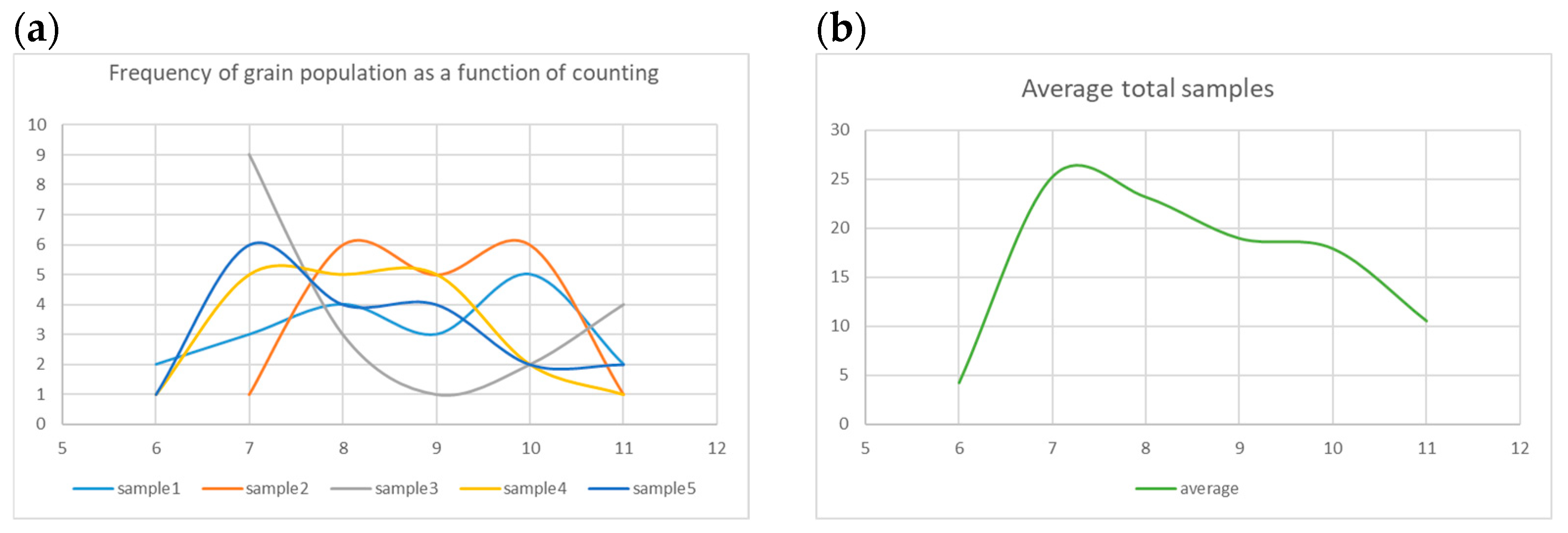
Figure 9a shows the grouping of the grain counting data along the horizontal axis; here, it is possible to see that the grain count remains mainly between the mean centered values, as can be confirmed in Figure 9b. There are only a few minimum and maximum values; the major quantity of values are in the middle of the curve. There are two centered tops on the curve, but the dispersion of data is not significant. Thus, the grain populations also remain homogeneous along the horizontal axis, although these are very near and the major area is below these values. In these figures, the populations of grains counted are shown on the horizontal axis, and the vertical axis represents the frequency of these measurements. In consequence, for all samples the grain size increases as the number of grains counted decreases (in other words, grain size increases from right to left).

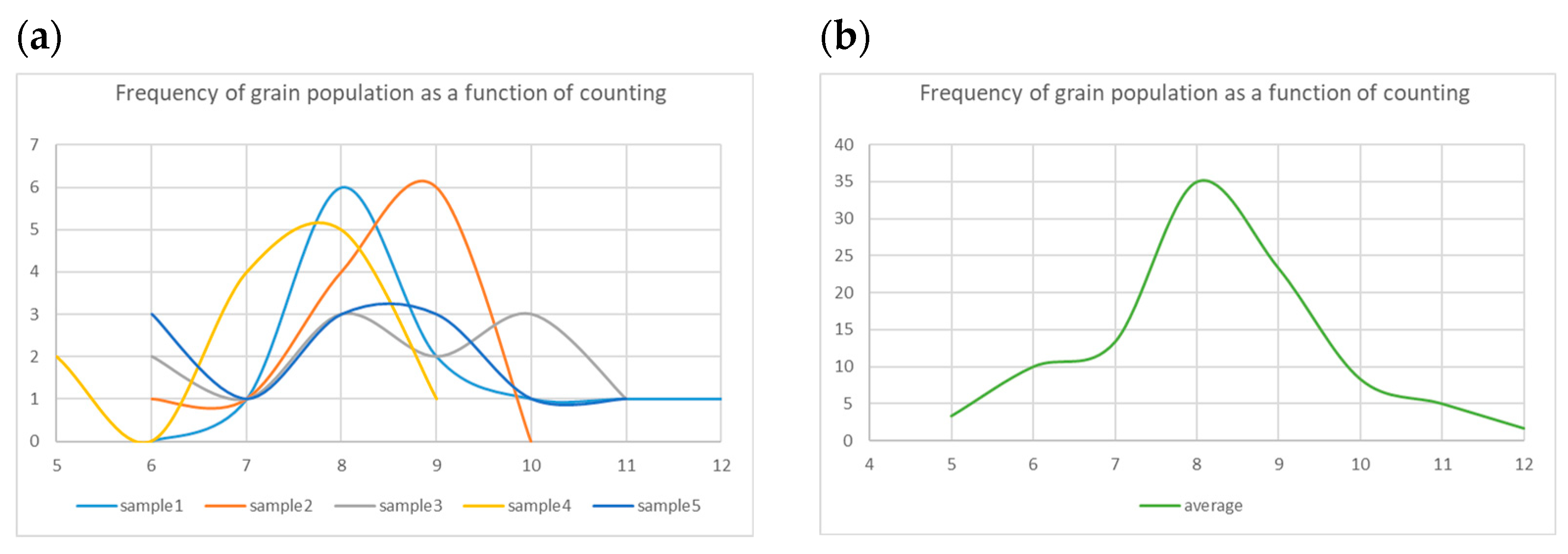
Figure 10a shows the same analysis performed in Figure 9a, but the analysis is for the vertical axis. Here, all samples again have a centered grain size; therefore, the grain size is almost the same along this axis. There is a homogenous distribution with the exception of sample 3 which shows a large population of grains with a size between slightly small and medium in size. The behavior of this sample has a quasi-parabolic form; consequently, in this sample there are some populations of grains that are slightly small and slightly large. This influence can be clearly appreciated in Figure 10b where there is a light tendency of grains to be just a little below the mean size.

Figure 11a shows the same procedure for the radial counting procedure performed. Here again, the grain populations were grouped, and again a tendency to remain near the mean grain size value can be appreciated in all samples with a centered grain population; therefore, there are only a few grains that are very small and a few that are very large. Here, there is a mean, a median, and a mode relatively concurrent with an evident single top value. The averaged curve in Figure 11b shows a single top value without a clearly defined bias.

7. Comparison Between Simulated and Real Samples

In order to obtain a valid relation value between real and simulated samples, Equation (13) was solved; the results indicate the portion in μm in the real samples that represents every single pixel in the simulated sample.

$${\displaystyle \frac{g_{size \left(\mathrm{p}\mathrm{i}\mathrm{x}\mathrm{e}\mathrm{l}\mathrm{s}\right)}}{g_{size \left(\mu \mathrm{m}\right)}}}={\displaystyle \frac{867.21 \mathrm{p}\mathrm{i}\mathrm{x}\mathrm{e}\mathrm{l}\mathrm{s}}{752.7 \mathsf{\mu }\mathrm{m}}}=1.152$$

(13)

The grains in the rectangular and square real samples are 97.903 and 74.338, respectively, and the grains in the simulated sample are 276.75; thus, the size relations with the real samples are 3.723 and 2.827. Therefore, the simulated sample is bigger in those proportions, which is another geometrical similarity between the samples. Moreover, in Figure 12, there is a region cut from a computationally simulated sample using the inverse with 1/3.723 that can be assumed to be a representation of a real sample.

Dendritic evolution is not considered in this work; because the simulation of this phenomenon involves modification towards a minor scale, here only consolidated solidified flat fronts are simulated [9,13,14,15,29,30,31,32,34,35,36]. Although we know that many phenomena occur during metal solidification, such as micro segregation, the distribution of solutions, and inclusion, entrapment, etc., these are challenges we are planning to overcome in future works.

Some of the present authors have worked with thermal gradients and heat removal phenomena in steel billets. These factors effectively directly affect grain structure formation, especially where transitions zones modify grain morphology; consequently, the characterization and comparisons must be conducted zone by zone. This problem appears when heat removal is involved in solving solidification [11,12,21,40,41,42,43,44].

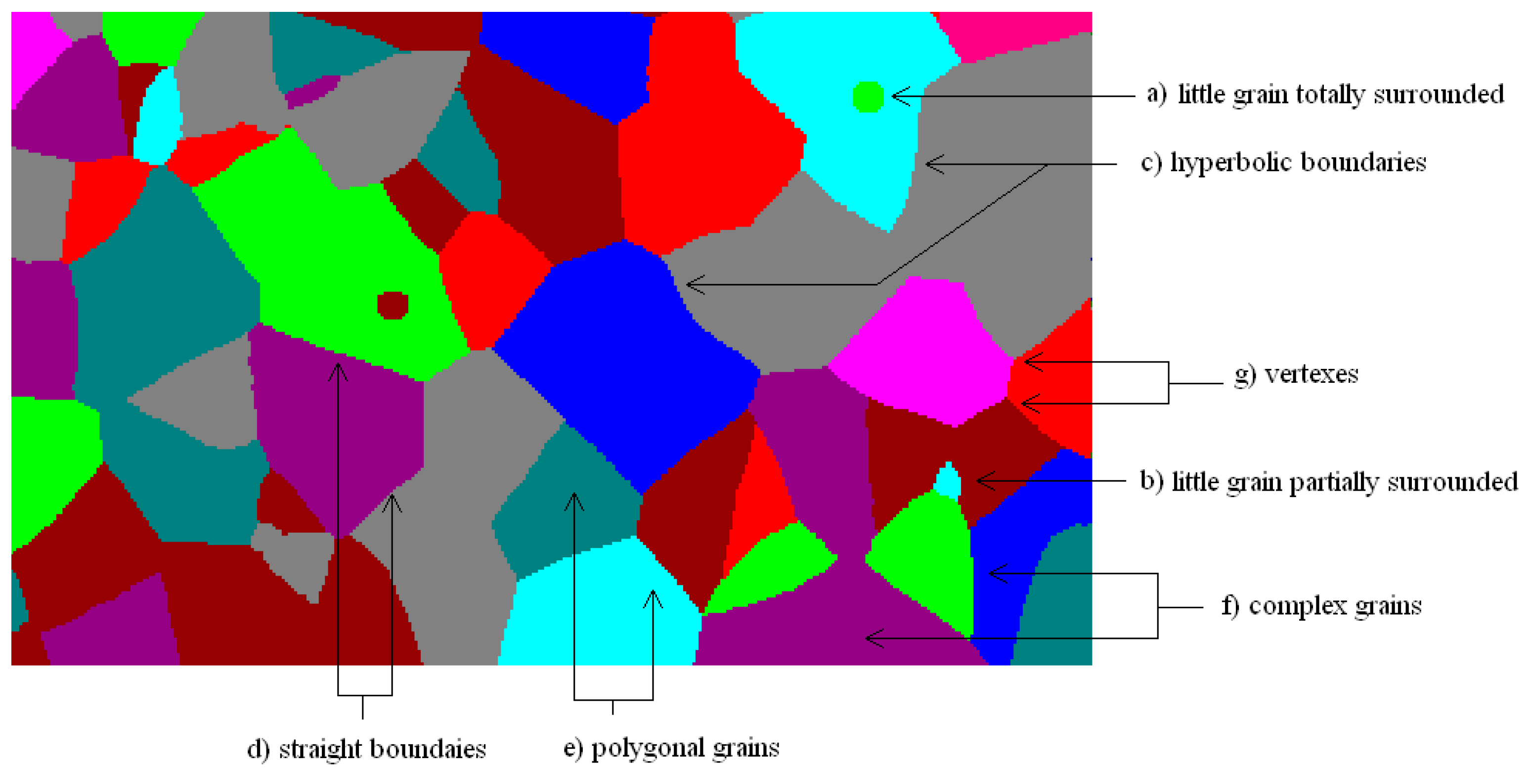
Finally, in Figure 13, a representative region of a computationally simulated sample is shown, evidencing some features of the sample that can be appreciated. Here, polygonal and complexed grains can be identified, and the boundaries and vertexes can also be recognized. Moreover, the formation of complex boundaries, straight and hyperbolic, can also be found. Moreover, large and small grain sizes can be found with some detail; for example, as a consequence of grain nucleation and growth, there are some little grains partially and totally surrounded by other bigger grains.

The potential applications of this research in materials science are focused on our understanding of the nucleation and growth mechanisms needed to form grains and how to establish valid rules to know the influence of the parameters on any grain structure; moreover, future works should also focus on the validation of the models developed with transition zones, in other words where the equiaxed grains change toward a columnar form, and explaining the influence of heat removal on metal solidification.

8. Conclusions

The procedure for the characterization of the real samples was appropriately applied and demonstrated to be effective in obtaining feasible values from measurements; the computational tools were also demonstrated to be adequate for the characterization of the computationally simulated samples.

Geometrical similarities between the real and simulated samples were successfully proved, evidencing similar grain sizes, similar grain populations, and similar distributions around the samples. The grains counted were proportional and the grain sizes were very similar. Consequently, the same grain morphology was observed on the real samples’ rectangular and square analyzed areas; then, these were compared with simulated samples. It must be mentioned that for the simulated samples, we did not consider a preferential growth process; thus, an equiaxed morphology resulted and only a single nucleation operation was defined. In consequence, the structure resulted from an initial definition of nucleated points which included growth all around themselves.

Grain structures simulated computationally and real metallic samples were polygonal and equiaxed with some complex grains; thus, both were also geometrically similar. Detailing and establishing geometrical values for the evidenced similarities was also conducted, verified, and discussed.