Dissipation of Energy in a Compressible Nematic Microvolume Under Effect of a Temperature Gradient

Abstract

We have carried out a numerical study of hydrodynamic processes in the hybrid-aligned channel of a compressible liquid crystal (HACLC) under the effect of a temperature gradient $\nabla T$ applied across a liquid crystal film. Calculations based on the classical Leslie–Ericksen theory showed that under the effect of $\nabla T$, the HACLC sample settles down to a stationary flow regime with both horizontal u and vertical w components of velocity $\mathbf{v}$, and the direction and magnitude of $\mathbf{v}$ are strongly effected by the direction of $\nabla T$. Calculations also showed that the relaxation of the stress tensor components ${\sigma }_{\mathrm{ij}}(z,t)(\mathrm{i},\mathrm{j}=\mathrm{x},\mathrm{z})$ in the hybrid-aligned compressible nematic microvolume is determined by the direction and magnitude of the thermomechanical force.

1. Introduction

A liquid drop of macrosized volume placed between two horizontal solid surfaces, if heated from below, develops a buoyancy force due to the volume expansion of the fluid near the bottom. For sufficiently strong heating, when heat is transported only by heat conduction, the buoyancy force may overcome the viscous force and the liquid drop starts moving in the horizontal plane. One such example is the Rayleigh–Benard instability in a horizontal layer of anisotropic fluid heated from below. When the temperature gradient increases, at a critical value, and the static thermal diffusion can no longer transfer the thermal energy, then a macroscopic fluid flow occurs. This disturbance of mechanical balance occurs due to a local difference in buoyancy caused by the inhomogeneous thermal expansion of the fluid. As a result, dissipative roll patterns may occur in the horizontal layer. When the gradient is further increased, the flow develops into a nonperiodic flow. This dissipative system is characterized by complex interaction between the convective flow and structural deformations and the flowing material is not necessarily a simple molecular liquid but is often a complex fluid, such as the liquid crystal (LC) [1] or a living organism. Understanding the dissipation processes in LC systems under the influence of the temperature gradient is essential knowledge in material science and is of fundamental interest. While much is known in LC systems about dissipation processes in LC systems under the influence of both electric and magnetic fields, relatively little is known about the effect of these fields on the LC phases confined in a micro- or nanosized volume. The manipulation of tiny amounts of molecular liquids in channels ranging in size from tens to hundreds of micrometers has emerged as a separate field called microfluidics [2,3]. Microfluidics has become a paradigm in various fields from chemical synthesis and biological analysis to optics and information technology [4,5,6]. Central to the success of microfluidics is the development of innovative methods for the manipulation of LC systems in microchannels. Traditionally, an external electric field is used for controlling fluid motion [7,8,9]. On the other hand, microvolumes of LC materials are extremely sensitive to both the temperature gradient $\nabla T$ and boundary conditions, and, consequently, these factors, together with the anchoring forces, can influence the nature of hydrodynamic flow $\mathbf{v}$ in micro- or nanosized LC channels [10,11]. By the way, reducing the size of the channels to the nanoscale ensures a close connection between the nematic and biological fluids [4,6,12].

Recently, the problem of the motion of an ultra-thin (a few microliters) incompressible LC drop confined in the microsized volume between two horizontal and two lateral surfaces and subjected to uniform heating from below and above has been considered [10,11]. It has been shown that in the heat conduction regime the magnitude of the hydrodynamic flow $\mathbf{v}$ excited by $\nabla T$ in the hybrid-aligned incompressible nematic (HAIN) channel, is proportional $v\sim {\displaystyle \frac{d}{\eta }}{\sigma }_{zx}^{tm}$ to the tangential component of the thermomechanical stress tensor ${\sigma }_{zx}^{tm}$, where d and $\eta$ are the thickness and viscosity of LC material [10,11], respectively. The direction of $\mathbf{v}$ is influenced both by the direction of the heat flux $\mathbf{q}=-T{\displaystyle \frac{\delta \mathcal{R}}{\delta \nabla T}}$ and the character of the preferred anchoring of the director $\widehat{\mathbf{n}}$ to the restricted surfaces [10,11]. Here, $\mathcal{R}$ is the Rayleigh dissipation function of LC system.

In an attempt to make the next step towards the theoretical description of dissipation processes in confined compressible LCs under the influence of $\nabla T$, we performed a numerical study of evolution not only of the stress tensor components of compressible fluid but also the redistribution of the velocity fields. To calculate it, one must include the equation of state and the equation for the velocity $\mathbf{v}$, as well as consider the coupled director–velocity equations in the framework of the well-established Leslie–Ericksen theory [13,14], as well as the thermoconductivity equation for the temperature field $T(\mathbf{r},t)$ [15].

It should be noted that the horizontal layer of a resting LC fluid, heated from below, becomes unstable to convection due to the Rayleigh–Benard mechanism in the case when the driving force is not large enough to create convection. In this case, instability occurs at the value of $R=R_c\sim 1708$, regardless of the liquid under consideration [16]. Considering the size of an LC channel to be $\sim 10$–20 µm, in our case $R\ll R_c$; in the future, we will focus primarily on the thermal conductivity mode as in HAIN and hybrid-aligned compressible nematic (HACN) channels.

The outline of this paper is as follows: The system of hydrodynamic equations describing both director motion and fluid flow of a compressible LC phase confined between two bounding surfaces, accounting for the heat conduction, caused by heating both from below or above, is given in Section 2. Numerical results for the relaxation regimes, caused by the vertical temperature gradient, describing orientational relaxation of the director, velocity, and stress tensor components, are given in Section 3. Conclusions are summarized in Section 4.

2. Formulation of the Balance Equations for Compressible Nematic Fluids

First of all, we would like to focus on describing the temperature T, density $\rho$, velocity $\mathbf{v}$, and director $\widehat{\mathbf{n}}$ distributions that are produced in a two-dimensional (2D) microsized compressible nematic (CN) channel under the effect of a temperature gradient $\nabla T$. Consider the 2D HACN volume, which is bounded by two infinitely long boundaries at a distance of d on a scale of the order of tens micrometers and is initially at rest. Assuming that the temperature gradient $\nabla T$ changes only in the z direction, which coincides with the direction of the unit vector $\widehat{\mathbf{k}}$ directed from the lower substrate to the upper one, we can assume that the components of the director $\widehat{\mathbf{n}}=sin\theta (z,t)\widehat{\mathbf{i}}+cos\theta (z,t)\widehat{\mathbf{k}}$, as well as other physical quantities, depend only on the coordinate z and time t. Here $\theta$ denotes the polar angle, i.e., the angle between the direction of the director $\widehat{\mathbf{n}}$ and the unit vector $\widehat{\mathbf{k}}$, while the unit vector $\widehat{\mathbf{i}}$ is directed parallel to the lower substrate, and $\widehat{\mathbf{j}}=\widehat{\mathbf{k}}\times \widehat{\mathbf{i}}$, respectively. If the HACN volume, with the homeotropic aligning of the director field ${\widehat{\mathbf{n}}}_{z=0}\Vert \widehat{\mathbf{k}}$ on the lower, and planar ${\widehat{\mathbf{n}}}_{z=d}\Vert \widehat{\mathbf{i}}$, on the upper bounding surfaces is heated from below or above, due to the coupling between $\nabla T$ and $\nabla \widehat{\mathbf{n}}$ in this LC volume, the hydrodynamic flow $\mathbf{v}(z,t)=v_x(z,t)\widehat{\mathbf{i}}+v_z(z,t)\widehat{\mathbf{k}}=u(z,t)\widehat{\mathbf{i}}+w(z,t)\widehat{\mathbf{k}}$ is exited.

The 2D hybrid alignment of the compressible nematic film confined between two solid surfaces suggests that

$$\begin{array}{c}\hfill \theta {\left(z\right)}_{\mathrm{z}=0}=0,\theta {\left(z\right)}_{\mathrm{z}=\mathrm{d}}={\displaystyle \frac{\pi }{2}},\end{array}$$

(1)

and its initial orientation is perturbed to be tilted with respect to the interface, with

$$\begin{array}{c}\hfill \theta (z,t=0)={\displaystyle \frac{\pi }{2d}}z,\end{array}$$

(2)

and then allowed to relax to its equilibrium value ${\theta }_{\mathrm{eq}}\left(z\right)$. In turn, the velocity on these surfaces has satisfied the no-slip boundary condition

$$\begin{array}{c}\hfill u{\left(z\right)}_{\mathrm{z}=0}=0,u{\left(z\right)}_{\mathrm{z}=\mathrm{d}}=0,\\ \hfill w{\left(z\right)}_{\mathrm{z}=0}=0,w{\left(z\right)}_{\mathrm{z}=\mathrm{d}}=0.\end{array}$$

(3)

Here, we consider two cases, firstly, when the upper surface is hotter than the lower one, and the boundary condition for the temperature field must satisfy

$$\begin{array}{c}\hfill T_{\mathrm{z}=\mathrm{d}}=T_{\mathrm{up}}=T_2,T_{\mathrm{z}=0}=T_{\mathrm{lw}}=T_1,\\ \hfill T_2>T_1\left(\mathrm{CASE}\mathrm{I}\right)\end{array}$$

(4)

and secondly, when the lower surface is hotter than the upper one, and the boundary condition for the temperature field must satisfy

$$\begin{array}{c}\hfill T_{\mathrm{z}=\mathrm{d}}=T_{\mathrm{up}}=T_2,T_{\mathrm{z}=0}=T_{\mathrm{lw}}=T_1,\\ \hfill T_2<T_1\left(\mathrm{CASE}\mathrm{II}\right),\end{array}$$

(5)

respectively. Thus, solid surfaces are kept at different temperatures, and the HACN film is exposed to the temperature gradient $\nabla T$ directed parallel to the unit vector $\widehat{\mathbf{k}}$.

Now, the reorientation of director field $\widehat{\mathbf{n}}$ in the HACN film, confined between two solid surfaces, under the effect of the temperature gradient $\nabla T$, when the relaxation regime is governed by viscous, elastic, and thermomechanical forces with accounting for hydrodynamic flow $\mathbf{v}$, can be obtained by solving a system consisting of mass, torque, momentum, and entropy balance equations.

If we assume that the liquid is compressible, then the mass balance equation will take the form

$$\begin{array}{c}\hfill {\rho }_{,\mathrm{t}}+\nabla ·\left(\rho \mathbf{v}\right)=0,\end{array}$$

(6)

where ${\rho }_{,\mathrm{t}}=\partial \rho (z,t)/\partial t$. In turn, the torque balance equation gives us the equation for the reorientation of the director field, which in our case will take the form

$$\begin{array}{c}\hfill {\mathbf{T}}_{\mathrm{el}}+{\mathbf{T}}_{\mathrm{vis}}+{\mathbf{T}}_{\mathrm{tm}}=0,\end{array}$$

(7)

where ${\mathbf{T}}_{\mathrm{el}}={\displaystyle \frac{\delta {\mathcal{W}}_{\mathrm{el}}}{\delta \widehat{\mathbf{n}}}}\times \widehat{\mathbf{n}}$ is the elastic, ${\mathbf{T}}_{\mathrm{vis}}={\displaystyle \frac{\delta {\mathcal{R}}^{\mathrm{vis}}}{\delta {\widehat{\mathbf{n}}}_{,\mathrm{t}}}}\times \widehat{\mathbf{n}}$ is the viscous, and ${\mathbf{T}}_{\mathrm{tm}}={\displaystyle \frac{\delta {\mathcal{R}}^{\mathrm{tm}}}{\delta {\widehat{\mathbf{n}}}_{,\mathrm{t}}}}\times \widehat{\mathbf{n}}$ is the thermomechanical torques, respectively. Here, ${\mathcal{W}}_{\mathrm{el}}$ is the elastic energy, while ${\mathcal{R}}^{\mathrm{vis}}$ and ${\mathcal{R}}^{\mathrm{tm}}$ are the viscous and thermomechanical contributions to the total Rayleigh dissipation function. (For details, see Appendix A.)

The linear momentum equation for the velocity field $\mathbf{v}$ can be written as [10,11]

$$\begin{array}{c}\hfill \rho {\displaystyle \frac{d\mathbf{v}}{dt}}=\nabla ·\sigma ,\end{array}$$

(8)

where the material derivative is ${\displaystyle \frac{dv}{dt}}=v_{,\mathrm{t}}+w{w}_{,\mathrm{z}}$, while the stress tensor (ST) $\sigma ={\sigma }^{\mathrm{el}}+{\sigma }^{\mathrm{vis}}+{\sigma }^{\mathrm{tm}}-P\mathcal{I}$ is the sum of elastic, viscous, thermomechanical parts and pressure and can be derived directly from the elastic contribution to energy and the Rayleigh dissipation function as ${\sigma }^{\mathrm{el}}=-{\displaystyle \frac{\partial {\mathcal{W}}_{\mathrm{el}}}{\partial \nabla \widehat{\mathbf{n}}}}·{\left(\nabla \widehat{\mathbf{n}}\right)}^{\mathrm{T}}$, ${\sigma }^{\mathrm{vis}}={\displaystyle \frac{\delta {\mathcal{R}}^{\mathrm{vis}}}{\delta \nabla \mathbf{v}}}$, and ${\sigma }^{\mathrm{tm}}={\displaystyle \frac{\delta {\mathcal{R}}^{\mathrm{tm}}}{\delta \nabla \mathbf{v}}}$, for the elastic, viscous, and thermomechanical contributions, respectively. Here, $w_{,\mathrm{z}}=\partial w(z,t)/\partial z$ is the partial derivative of vertical component velocity with respect to z.

The viscous contribution to the total pressure P is given by $P={\sigma }^v:\mathcal{I}={\sigma }_{xx}^v+{\sigma }_{zz}^v$, while the elastic contribution to P is equal to $P^{el}={\sigma }^{el}:\mathcal{I}={\sigma }_{xx}^{el}+{\sigma }_{zz}^{el}=-2W_F$, where $W_F={\displaystyle \frac{1}{2}}\left(K_1{n}_{z,z}^2+K_3{n}_{x,z}^2\right)$, respectively. Here, $\mathcal{I}$ is the unit tensor, and equations for the tensor components ${\sigma }_{xx}^v$ and ${\sigma }_{zz}^v$ are given in Appendix A.

When the temperature gradient $\nabla T(\sim 1.0[K/\mu m\left]\right)$ is set up, we expect that the temperature field $T(z,t)$ satisfies the heat conduction equation [10,11]

$$\begin{array}{c}\hfill C_{\mathrm{p}}{\left(\rho T\right)}_{,\mathrm{t}}=-q_{\mathrm{z},\mathrm{z}},\end{array}$$

(9)

where $C_{\mathrm{p}}$ is the heat capacity, $q_{\mathrm{z}}=-T{\displaystyle \frac{\delta \mathcal{R}}{\delta T_{,\mathrm{z}}}}$ is the heat flux in the HACN channel directed parallel to the unit vector $\widehat{\mathbf{k}}$, while $q_{\mathrm{z},\mathrm{z}}=\partial q_{\mathrm{z}}/\partial z$, respectively. Taking into account that $\widehat{\mathbf{n}}=sin\theta (z,t)\widehat{\mathbf{i}}+cos\theta (z,t)\widehat{\mathbf{k}}$ and $\mathbf{v}(z,t)=v_x(z,t)\widehat{\mathbf{i}}+v_z(z,t)\widehat{\mathbf{k}}=u(z,t)\widehat{\mathbf{i}}+w(z,t)\widehat{\mathbf{k}}$, the last equation can be rewritten in the form as

$$\begin{array}{c}\hfill C_{\mathrm{p}}{\left(\rho T\right)}_{,\mathrm{t}}={\lambda }_{\perp }{\left[T_{,\mathrm{z}}\left(\lambda {cos}^2\theta +{sin}^2\theta \right)\right]}_{,\mathrm{z}}+\\ \hfill \xi {\left[{\theta }_{,\mathrm{z}}T\left({\theta }_{,\mathrm{t}}({\displaystyle \frac{1}{2}}+{sin}^2\theta )-u_{,\mathrm{z}}{sin}^2\theta (1+{\displaystyle \frac{1}{2}}{sin}^2\theta )\right)\right]}_{,\mathrm{z}}-{\displaystyle \frac{\xi }{4}}{\left[T{w}_{,\mathrm{z}}{\theta }_{,\mathrm{z}}sin2\theta \right]}_{,\mathrm{z}},\end{array}$$

(10)

where $\lambda ={\lambda }_{\Vert }/{\lambda }_{\perp }$ and $\xi \sim {10}^{-12}J/mK$ is the thermomechanical constant [10,11]. Note that the density $\rho$, pressure P, and the temperature T of the liquid crystal system are connected by an equation of state, which in our case takes the form of a·“Boussinesq approximation” [17]

$$\begin{array}{c}\hfill \rho ={\rho }_0\left(1-\alpha (T-T_1)\right),\end{array}$$

(11)

where $\alpha ={\displaystyle \frac{1}{\rho }}{\left({\displaystyle \frac{\partial \rho }{\partial T}}\right)}_P$ is the volume expansion coefficient and ${\rho }_0$ is the mass density of the LC phase.

In the case of the 2D compressible LC phase, the balance equations of dimensionless mass, torque, momentum, and entropy can be written inthe following forms. First of all, the condition of dimensionless compressibility (6) can be rewritten as

$$\begin{array}{c}\hfill -{\chi }_{,ø}-{\chi }_{,\mathrm{z}}w-(\chi -{\chi }_1)w_{,\mathrm{z}}+{\displaystyle \frac{1}{{\delta }_1}}{w}_{,\mathrm{z}}=0,\end{array}$$

(12)

where $\chi (z,\tau )=T(z,\tau )/T_{\mathrm{NI}}$ is the dimensionless temperature, $T_{\mathrm{NI}}$ is the nematic–isotropic transition temperature, ${\chi }_1=T_1/T_{\mathrm{NI}}$, $\tau =(K_{10}/{\gamma }_{10}{d}^2)t$ is the dimensionless time, ${\delta }_1=T_{\mathrm{NI}}\alpha$ is the parameter of the LC system, while $\overline{z}=z/d$ and $\overline{w}={\displaystyle \frac{{\gamma }_{10}{d}^2}{K_{10}}}w$ are the dimensionless distance away from the lower solid surface, and the vertical dimensionless component of velocity, respectively. Note that the overbars in the space variable z and the velocity component w have been eliminated. (For details, see Appendix A).

In turn, the dimensionless torque balance Equation (7) can be written as

$$\begin{array}{c}\hfill {\gamma }_1\left(\chi \right){\theta }_{,ø}=\mathcal{A}\left(\theta \right)u_{,\mathrm{z}}+{\left(\mathcal{G}\left(\theta \right){\theta }_{,\mathrm{z}}\right)}_{,\mathrm{z}}-{\displaystyle \frac{1}{2}}{\mathcal{G}}_{,\theta }\left(\theta \right){\theta }_{,\mathrm{z}}^2-{\delta }_2{\chi }_{,\mathrm{z}}{\theta }_{,\mathrm{z}}\left({\displaystyle \frac{1}{2}}+{sin}^2\theta \right),\end{array}$$

(13)

where ${\overline{\gamma }}_1\left(\chi \right)={\gamma }_1\left(\chi \right)/{\gamma }_{10}$ is the dimensionless rotational viscosity coefficient (RVC), $u_{,\mathrm{z}}=\partial u(z,\tau )/\partial z$, $\mathcal{A}\left(\theta \right)=\overline{\mathcal{A}}\left(\theta \right)/{\gamma }_{10}={\displaystyle \frac{1}{2}}\left({\gamma }_1\left(\chi \right)-{\gamma }_2\left(\chi \right)cos2\theta \right)/{\gamma }_{10}$, $\mathcal{G}\left(\theta \right)=(K_1\left(\chi \right)$${sin}^2\theta +K_3\left(\chi \right){cos}^2\theta )/K_{10}$, ${\mathcal{G}}_{,\theta }\left(\theta \right)$ is the derivative of $\mathcal{G}\left(\theta \right)$ with respect to $\theta$, and ${\delta }_2=\xi T_{NI}/K_{10}$ is the parameter of the system, respectively. Here, $\xi \sim {10}^{-12}J/mK$ is the thermomechanical constant [10,11], and the overbar in RVC ${\overline{\gamma }}_1\left(\chi \right)$ has been eliminated. (For details, see Appendix A).

In the case of compressible fluid, the dimensionless momentum balance Equation (8) reduces to

$$\begin{array}{c}\hfill {\delta }_3{\left[\left(1-{\delta }_1(\chi -{\chi }_1)\right)u\right]}_{,ø}=\\ \hfill {\left[\overline{h}\left(\theta \right)u_{,\mathrm{z}}-\mathcal{A}\left(\theta \right){\theta }_{,ø}-{\delta }_2{\chi }_{,\mathrm{z}}{\theta }_{,\mathrm{z}}{sin}^2\theta \left(1+{\displaystyle \frac{1}{2}}{sin}^2\theta \right)+{\displaystyle \frac{{\overline{\beta }}_0}{6}}{w}_{,\mathrm{z}}sin2\theta \right]}_{,\mathrm{z}},\end{array}$$

(14)

and

$$\begin{array}{c}\hfill {\delta }_3{\left[\left(1-{\delta }_1(\chi -{\chi }_1)\right)w\right]}_{,ø}=\\ \hfill {\left[{\displaystyle \frac{{\overline{\beta }}_0}{6}}\left(u_{,\mathrm{z}}sin2\theta +{\displaystyle \frac{2}{3}}{w}_{,\mathrm{z}}\right)-{\displaystyle \frac{{\delta }_2}{4}}{\chi }_{,\mathrm{z}}{\theta }_{,\mathrm{z}}sin2\theta -{\displaystyle \frac{1}{2}}\mathcal{G}\left(\theta \right){\theta }_{,\mathrm{z}}^2\right]}_{,\mathrm{z}},\end{array}$$

(15)

respectively. Here, ${\delta }_3={\rho }_0{K}_{10}/{\gamma }_{10}^2$ is an additional parameter of the LC system. (For details, see Appendix A).

We also expect that the dimensionless temperature field $\chi (z,\tau )$ satisfies the heat conduction equation [10,11]

$$\begin{array}{c}\hfill {\delta }_4{\left[\left(1-{\delta }_5(\chi -{\chi }_1)\right)\chi \right]}_{,ø}={\left[{\chi }_{,\mathrm{z}}\left(\lambda {cos}^2\theta +{sin}^2\theta \right)\right]}_{,\mathrm{z}}+\\ \hfill {\delta }_5{\left[\chi {\theta }_{,\mathrm{z}}\left({\theta }_{,ø}({\displaystyle \frac{1}{2}}+{sin}^2\theta )-u_{,\mathrm{z}}{sin}^2\theta (1+{\displaystyle \frac{1}{2}}{sin}^2\theta )\right)-{\displaystyle \frac{1}{4}}{w}_{,\mathrm{z}}sin2\theta \right]}_{,\mathrm{z}},\end{array}$$

(16)

where ${\delta }_4={\rho }_0{C}_p{K}_{10}/\left({\gamma }_{10}{\lambda }_{\perp }\right)$ and ${\delta }_5=T_{\mathrm{NI}}{K}_{10}\xi /\left({\gamma }_{10}{\lambda }_{\perp }{d}^2\right)$ are two extra parameters of the LC system. Note that the overbars in the space variable z in the last four Equations (13)–(16) have also been eliminated. (For details, see Appendix A).

Now, the reorientation of the director in the LC film confined between two solid surfaces, when the relaxation regime is governed by the viscous, elastic, and thermomechanical forces, and with accounting for the flow, can be obtained by solving the system of the nonlinear partial differential Equations (12)–(16), with the appropriate boundary conditions for the polar angle $\theta$

$$\begin{array}{c}\hfill \theta {\left(z\right)}_{\mathrm{z}=0}=0,\theta {\left(z\right)}_{\mathrm{z}=1}={\displaystyle \frac{\pi }{2}},\end{array}$$

(17)

with the no-slip boundary condition for both velocities

$$\begin{array}{c}\hfill u{\left(z\right)}_{\mathrm{z}=0}=0,u{\left(z\right)}_{\mathrm{z}=1}=0,\\ \hfill w{\left(z\right)}_{\mathrm{z}=0}=0,w{\left(z\right)}_{\mathrm{z}=1}=0,\end{array}$$

(18)

and with the initial condition for the angle $\theta$ written in the form

$$\begin{array}{c}\hfill \theta (z,\tau =0)={\displaystyle \frac{\pi }{2}}z.\end{array}$$

(19)

Below, two cases are considered: first, when the upper surface is hotter than the lower one, and the boundary condition for the temperature field must satisfy

$$\begin{array}{c}\hfill {\chi }_{\mathrm{z}=1}={\chi }_{\mathrm{up}}={\chi }_2,{\chi }_{\mathrm{z}=0}={\chi }_{\mathrm{lw}}={\chi }_1,\\ \hfill {\chi }_2>{\chi }_1\left(\mathrm{CASE}\mathrm{I}\right),\end{array}$$

(20)

and, second, when the lower surface is hotter than the upper one, and the boundary condition for the temperature field must satisfy

$$\begin{array}{c}\hfill {\chi }_{\mathrm{z}=1}={\chi }_{\mathrm{up}}={\chi }_2,{\chi }_{\mathrm{z}=0}={\chi }_{\mathrm{lw}}={\chi }_1,\\ \hfill {\chi }_1>{\chi }_2\left(\mathrm{CASE}\mathrm{II}\right),\end{array}$$

(21)

respectively.

For the case of $4-n-pentyl-4^{\prime }-cyanobiphenyl$ $\left(5CB\right)$, at a temperature corresponding to the nematic phase, the values of the material constants are borrowed from the Ref. [10]. Thus, the mass density is $\sim {10}^3$ $kg/m^3$, $T_{\mathrm{NI}}\left(5CB\right)\sim 307$ K, and the highest values for elastic constants are $K_{10}\sim 13$ $pN$, $K_{30}\sim 19$ $pN$, and ${\gamma }_{10}\sim 0.077$ $Pas$, the specific heat $C_{\mathrm{p}}\sim {10}^3$ $J/kgK$, and the thermal conductivity coefficients ${\lambda }_{\Vert }\sim 0.24$ and ${\lambda }_{\perp }\sim 0.13$ $W/mK$, respectively. The value of the thermomechanical constant $\xi$ is equal to $\sim {10}^{-12}$ $J/m$ K, while the volume expansion coefficient $\alpha$ is equal to $\sim {10}^{-3}{K}^{-1}$, respectively. Thus, the set of parameters values, which are involved in Equations (12)–(16) are ${\delta }_1\sim 0.3$, ${\delta }_2\sim 24$, ${\delta }_3\sim 2\times {10}^{-6}$, ${\delta }_4\sim 6\times {10}^{-4}$, and ${\delta }_5\sim 2\times {10}^{-9}$, respectively. Using the fact that ${\delta }_3\ll 1$, the momentum balance Equations (14) and (15) can be considerably simplified as velocities following adiabatically the motion of the director. Thus, the whole left-hand side of Equations (14) and (15) can be neglected, reducing it to

$$\begin{array}{c}\hfill {\sigma }_{\mathrm{zx}}=\overline{h}\left(\theta \right)u_{,\mathrm{z}}-\mathcal{A}\left(\theta \right){\theta }_{,ø}-{\delta }_2{\chi }_{,\mathrm{z}}{\theta }_{,\mathrm{z}}{sin}^2\theta \left(1+{\displaystyle \frac{1}{2}}{sin}^2\theta \right)+{\displaystyle \frac{{\overline{\beta }}_0}{6}}{w}_{,\mathrm{z}}sin2\theta ={\mathcal{C}}_1\left(\tau \right),\end{array}$$

(22)

and

$$\begin{array}{c}\hfill {\sigma }_{\mathrm{zz}}={\displaystyle \frac{{\overline{\beta }}_0}{6}}\left(u_{,\mathrm{z}}sin2\theta +{\displaystyle \frac{2}{3}}{w}_{,\mathrm{z}}\right)-{\displaystyle \frac{{\delta }_2}{4}}{\chi }_{,\mathrm{z}}{\theta }_{,\mathrm{z}}sin2\theta -{\displaystyle \frac{1}{2}}\mathcal{G}\left(\theta \right){\theta }_{,\mathrm{z}}^2={\mathcal{C}}_2\left(\tau \right),\end{array}$$

(23)

respectively, where the functions ${\mathcal{C}}_1\left(\tau \right)$ and ${\mathcal{C}}_2\left(\tau \right)$ does not depends on z and will be fixed by the boundary conditions. Equation (16) also can be considerably simplified, because both parameters ${\delta }_4$, ${\delta }_5\ll 1$, and the whole left-hand side of Equation (16), as well as the second term, can be neglected so that Equation (16) takes the form

$$\begin{array}{c}\hfill {\left[{\chi }_{,\mathrm{z}}\left(\lambda {cos}^2\theta +{sin}^2\theta \right)\right]}_{,\mathrm{z}}=0.\end{array}$$

(24)

The last equation has a solution

$$\begin{array}{c}\hfill \chi (z,\tau )={\displaystyle \frac{\Delta \chi }{I}}{\int }_0^z{\left(\lambda {cos}^2\theta +{sin}^2\theta \right)}^{-1}dz+{\chi }_i,\end{array}$$

(25)

where $I={\int }_0^1{\left(\lambda {cos}^2\theta +{sin}^2\theta \right)}^{-1}dz$, $\Delta \chi ={\chi }_2-{\chi }_1$, and ${\chi }_i=T_i/T_{\mathrm{NI}}$, respectively.

Now, let us consider the rest stress tensor components ${\sigma }_{\mathrm{xz}}$ and ${\sigma }_{\mathrm{xx}}$, respectively. Having obtained ${\sigma }_{\mathrm{zx}}$ (see, Equation (22)), and using the relation ${\sigma }_{\mathrm{zx}}\left(\tau \right)-{\sigma }_{\mathrm{xz}}\left(\tau \right)=\partial \mathcal{R}\left(\tau \right)/\partial {\theta }_{,\tau }$, one can calculate the dimensionless stress tensor component ${\sigma }_{\mathrm{xz}}$, which takes the form

$$\begin{array}{c}\hfill {\sigma }_{\mathrm{xz}}\left(\tau \right)={\sigma }_{\mathrm{zx}}\left(\tau \right)-{\left(\mathcal{G}\left(\theta \right){\theta }_{,\mathrm{z}}\right)}_{,\mathrm{z}}+{\displaystyle \frac{1}{2}}{\mathcal{G}}_{\theta }\left(\theta \right){\theta }_{,\mathrm{z}}^2.\end{array}$$

(26)

In the case of planar geometry, the dimensionless pressure $P(z,\tau )={\displaystyle \frac{d^2}{K_{10}}}P(z,t)$ in the HACN channel is given by

$$\begin{array}{c}\hfill P(z,\tau )={\sigma }_{\mathrm{zz}}^{\mathrm{vis}}(z,\tau )={\sigma }_{\mathrm{xx}}^{\mathrm{vis}}(z,\tau ),\end{array}$$

(27)

whereas the full form of ${\sigma }_{\mathrm{xx}}$ is given by

$$\begin{array}{c}\hfill {\sigma }_{\mathrm{xx}}(z,\tau )={\sigma }_{\mathrm{xx}}^{\mathrm{vis}}(z,\tau )+{\sigma }_{\mathrm{xx}}^{\mathrm{el}}(z,\tau )=P(z,\tau ),\end{array}$$

(28)

which takes into account that ${\sigma }_{\mathrm{xx}}^{\mathrm{el}}=0$. Here, ${\sigma }^{\mathrm{vis}}={\displaystyle \frac{\delta {\mathcal{R}}^{\mathrm{vis}}}{\delta \nabla \mathbf{v}}}$ and ${\sigma }^{\mathrm{el}}=-{\displaystyle \frac{\partial {\mathcal{W}}_{\mathrm{el}}}{\partial \nabla \widehat{\mathbf{n}}}}·{\left(\nabla \widehat{\mathbf{n}}\right)}^{\mathrm{T}}$ are the viscous and elastic contributions to the full stress tensor $\sigma$, respectively.

3. Orientational Relaxation of Velocity and Stress Tensor Components in the HACN Channel

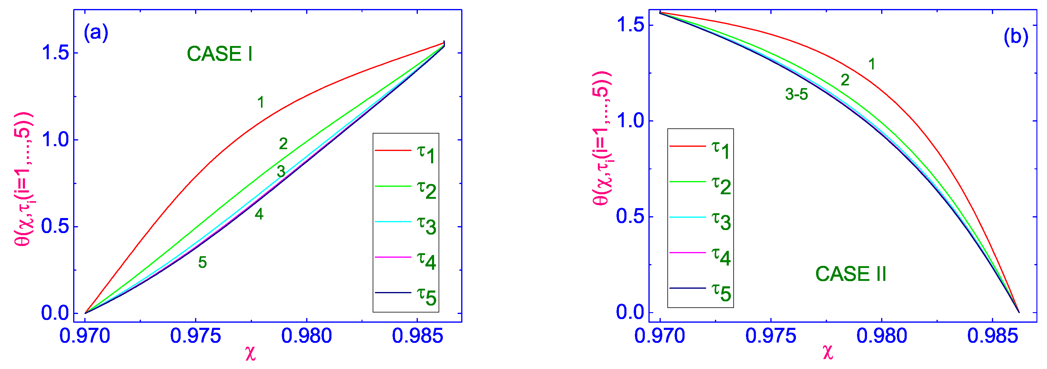
The relaxation of director $\widehat{\mathbf{n}}$ to its equilibrium orientation ${\widehat{\mathbf{n}}}_{\mathrm{eq}}$, which is described by the polar angle $\theta (z,\tau )$, from the initial condition $\theta (z,\tau =0)={\displaystyle \frac{\pi }{2}}z$ to ${\theta }_{\mathrm{eq}}$, for both cases I and II, is shown in Figure 1a and Figure 1b, respectively.

This was obtained by solving nonlinear partial differential Equations (13), (22), (23) and (25), together with the boundary conditions (17), (18), (20), and (21), as well as with the initial condition (19) by the numerical relaxation method [18]. In the calculations, the relaxation criterion $ϵ=|({\theta }_{(\mathrm{m}+1)}(z,\tau )-{\theta }_{\left(\mathrm{m}\right)}(z,\tau ))/{\theta }_{(\mathrm{m}+1)}(z,\tau )|$ was chosen to be equal to ${10}^{-4}$, and the numerical procedure was then carried out until a prescribed accuracy was achieved. Here, m is the iteration number and ${\tau }_R$ is the relaxation time.

In case I, as shown in Figure 1a, the initial convex profile of $\theta (\chi ,{\tau }_1)$ is converted into a set of concave profiles $\theta (\chi ,{\tau }_i(i=2,\cdots ,5))$, while in case II, as is shown in Figure 1b, the set of profiles $\theta (\chi ,{\tau }_i(i=1,\cdots ,5))$ is described by convex curves. Later, this difference in the behavior of $\theta (\chi ,{\tau }_i(i=1,\cdots ,5))$ profiles will be reflected in the different behavior of the velocity profiles, because we will be dealing with a different behavior of $\nabla \widehat{\mathbf{n}}$.

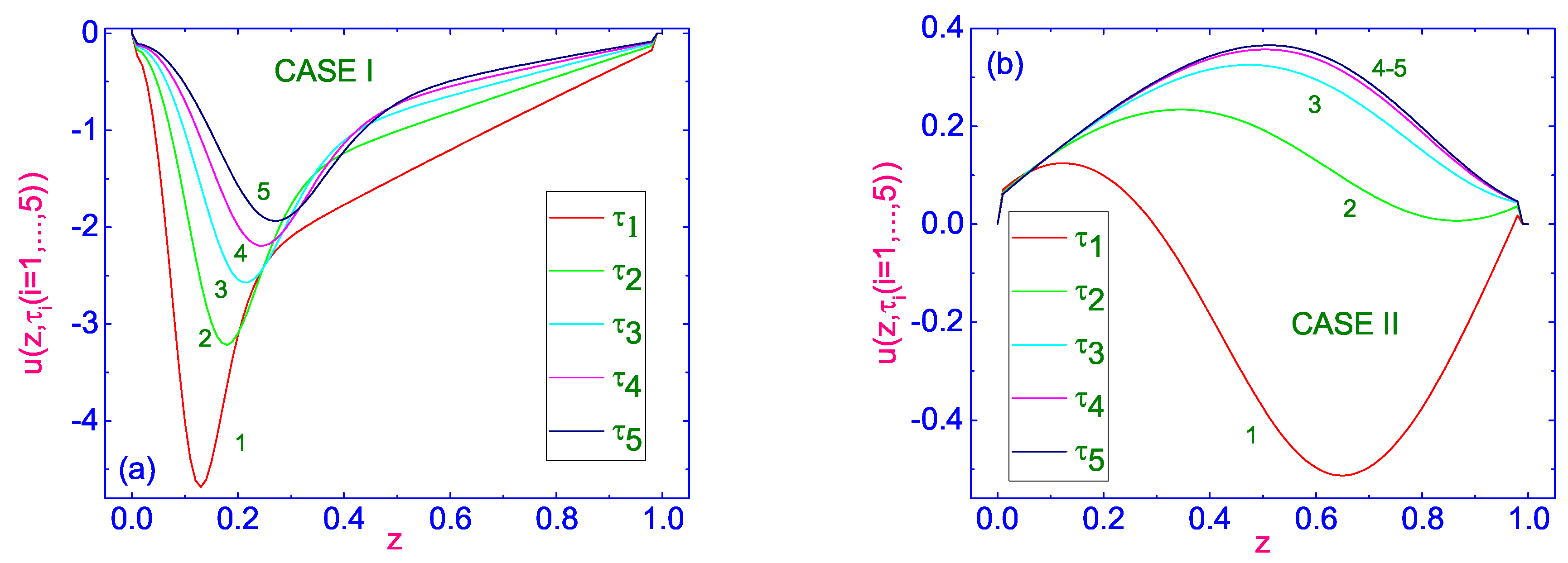
The horizontal component of velocity $v_x(z,{\tau }_i(i=1,\cdots ,5))\equiv u(z,{\tau }_i(i=1,\cdots ,5))$ as a function of the dimensionless distance z counted from the lower cooler ${\chi }_{\mathrm{z}=0}={\chi }_1$ to the upper warmer ${\chi }_{\mathrm{z}=1}={\chi }_1+\Delta \chi$ (case I) bounding surface, for the number of dimensionless times ${\tau }_i={\tau }_{0}i,(i=1,\cdots ,5)$, the values of which increase from the curve (1) to the curve (5), is shown in Figure 2a, while the same dependencies for case II are shown in Figure 2b, respectively.

In case I, when the LC sample is heated from above with the dimensionless temperature difference $\Delta \chi =0.0162$ ($\sim 5$ K), the profiles of the horizontal component $u(z,{\tau }_i(i=1,\cdots ,5))$ of velocity are characterized by monotonic decreasing of $u(z,{\tau }_i(i=1,\cdots ,5))$ with changing $\tau$, before getting the equilibrium distribution $u_{\mathrm{eq}}\left(z\right)$ across the LC channel. This distribution is characterized by the local maximum near the cooler lower boundary $u(z=0.27,{\tau }_5)=u_{\mathrm{eq}}(z=0.27)=1.94(35.5$ µm/s), and the horizontal component of velocity is directed in the negative direction. In case II, the evolution of velocity profiles is more complicated. In this case, as shown in Figure 2b, the initially concave profile of $u(z,{\tau }_1)$, with the horizontal velocity component directed in the negative direction is transformed into a set of convex profiles $u(z,{\tau }_i(i=2,\cdots ,5))$, with the horizontal component of the velocity directed in the positive direction. This distribution is characterized by the local maximum near the center of the LC sample $u(z=0.52,{\tau }_5)=u_{\mathrm{eq}}(z=0.52)=0.36(6.6$ µm/s), and the horizontal component of the velocity is directed in the positive direction. A simple comparison of the maximum values of $u_{\mathrm{eq}}(z=0.27)=1.94(35.5$ µm/s), in case I, and $u_{\mathrm{eq}}(z=0.52)=0.36(6.6$ µm/s), in case II, shows that in the first case, this value is almost 5 times greater than in the second case.

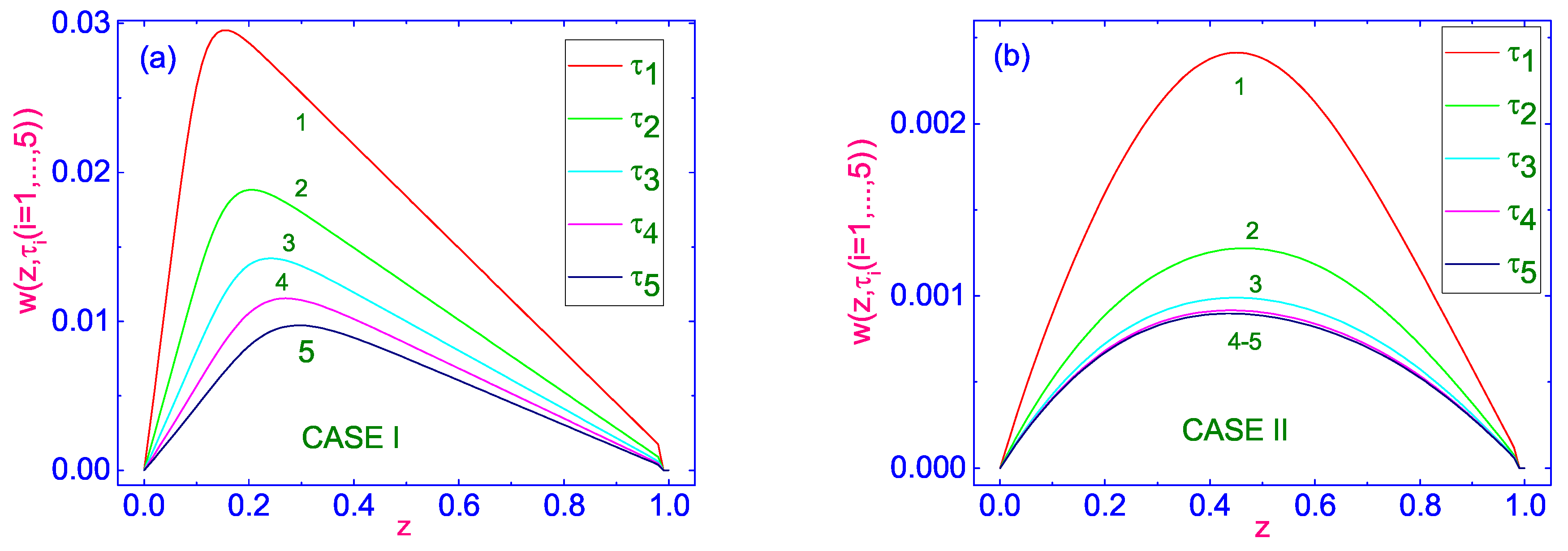
In turn, the vertical component of velocity $v_z(z,{\tau }_i(i=1,\cdots ,5))\equiv w(z,{\tau }_i(i=1,\cdots ,5))$ as a function of the dimensionless distance z counted from the lower cooler ${\chi }_{\mathrm{z}=0}={\chi }_1$ to the upper warmer ${\chi }_{\mathrm{z}=1}={\chi }_1+\Delta \chi$ (case I) bounding surface, for the number of dimensionless times ${\tau }_i={\tau }_{0}i,(i=1,\cdots ,5)$, the values of which increase from the curve (1) to the curve (5), are shown in Figure 3a, while the same dependencies, for case II are shown in Figure 3b, respectively.

In case I, when the LC sample is heated from above with the dimensionless temperature difference $\Delta \chi =0.0162$ (∼5K), the profiles of the vertical component $w(z,{\tau }_i(i=1,\cdots ,5))$ of velocity are characterized by monotonic decreasing of $w(z,{\tau }_i(i=1,\cdots ,5))$ with changing $\tau$, before getting the equilibrium distribution $w_{\mathrm{eq}}\left(z\right)$ across the LC channel. This distribution is characterized by the local maximum near the cooler lower boundary $w(z=0.3,{\tau }_5)=w_{\mathrm{eq}}(z=0.3)=0.01(0.2$ µm/s), and the vertical component of velocity is directed in the positive direction. In case II, the evolution of velocity profiles is also characterized by monotonic decreasing of $w(z,{\tau }_i(i=1,\cdots ,5))$ with changing $\tau$, before getting the equilibrium distribution $w_{\mathrm{eq}}\left(z\right)$ across the LC channel. In this case, as shown in Figure 3b, the set of convex profiles, the vertical component of velocity $w(z,{\tau }_1)$ is directed in the positive direction. This distribution is characterized by the local maximum near the center of the LC sample $w(z=0.46,{\tau }_5)=w_{\mathrm{eq}}(z=0.46)=0.0009(0.016$ µm/s), and the vertical component of the velocity is directed in the positive direction. A simple comparison of the maximum values of $w_{\mathrm{eq}}(z=0.3)=0.01(0.2$ m/s), in case I, and $w(z=0.46,{\tau }_5)=w_{\mathrm{eq}}(z=0.46)=0.0009(0.016$ m/s), in case II, shows that in the first case, this value is almost an order of magnitude greater than in the second case.

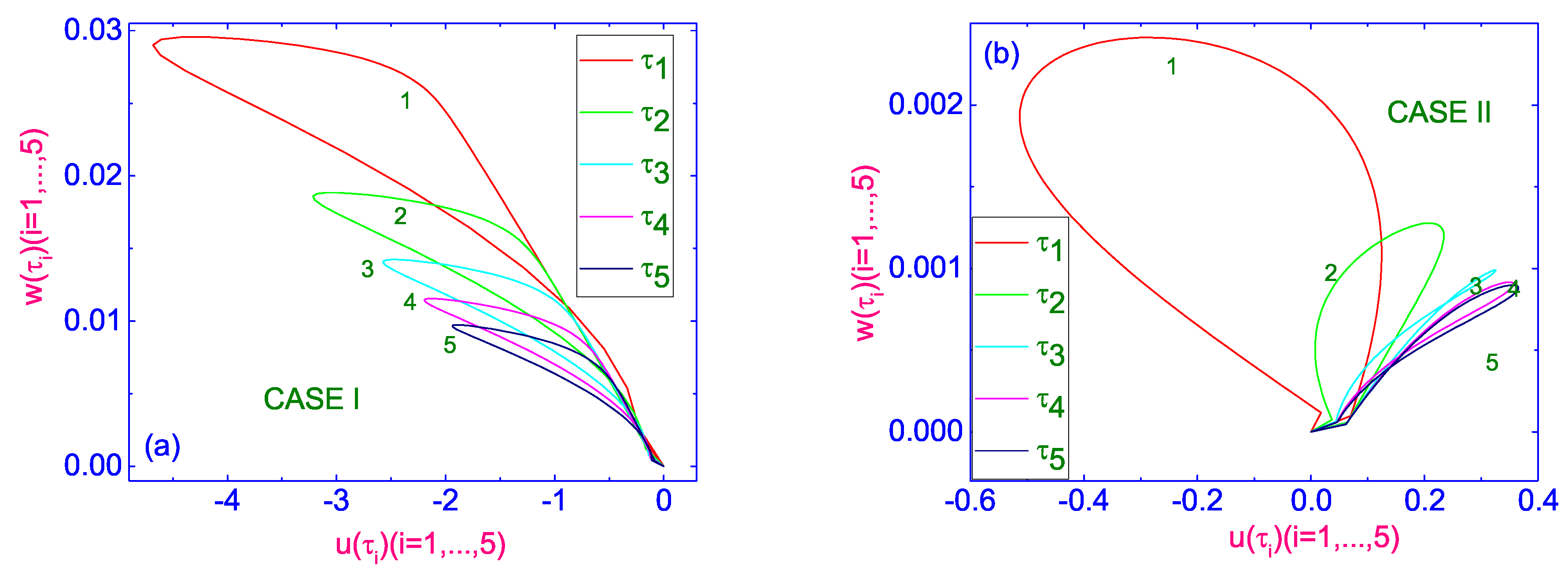
Finally, the evolution of $w-u$ diagram for the case of lower cooler (${\chi }_{z=0}={\chi }_1$) and upper hotter (${\chi }_{z=1}={\chi }_1+\Delta \chi$) bounding surfaces (case I), and for the number of dimensionless times ${\tau }_i={\tau }_{0}i,(i=1,\cdots ,5)$, whose values increase from curve (1) to curve (5), is shown in Figure 4a.

Here, ${\chi }_1=0.97$, $\Delta \chi =0.0162$ and ${\tau }_0=0.1$, respectively. This behavior is characterized by a monotonic decrease in the absolute values of both velocity components u and w, with the vertical component of the velocity directed in the positive direction, while the horizontal component is directed in the negative direction. When the LC sample is heated from below (case II), the evolution of $w-u$ diagram for the number of dimensionless times ${\tau }_i={\tau }_{0}i,(i=1,\cdots ,5)$, whose values increase from curve (1) to curve (5), is shown in Figure 4b. In this case, the evolution of $w-u$ diagram is more complicated. During the first time period, up to ${\tau }_1=0.1$, the horizontal component of the velocity $u\left({\tau }_1\right)$ changed direction from negative to positive, while during the subsequent time interval ${\tau }_5-{\tau }_1=0.4$, the evolution of $w-u$ diagram is characterized by a monotonous increase in the values of u, and by simultaneously increasing the value of w.

It should be noted that in cases I and II, hydrodynamic flows of different magnitude and direction are formed in the LC channel under the influence of the same temperature gradient $\nabla \chi$.

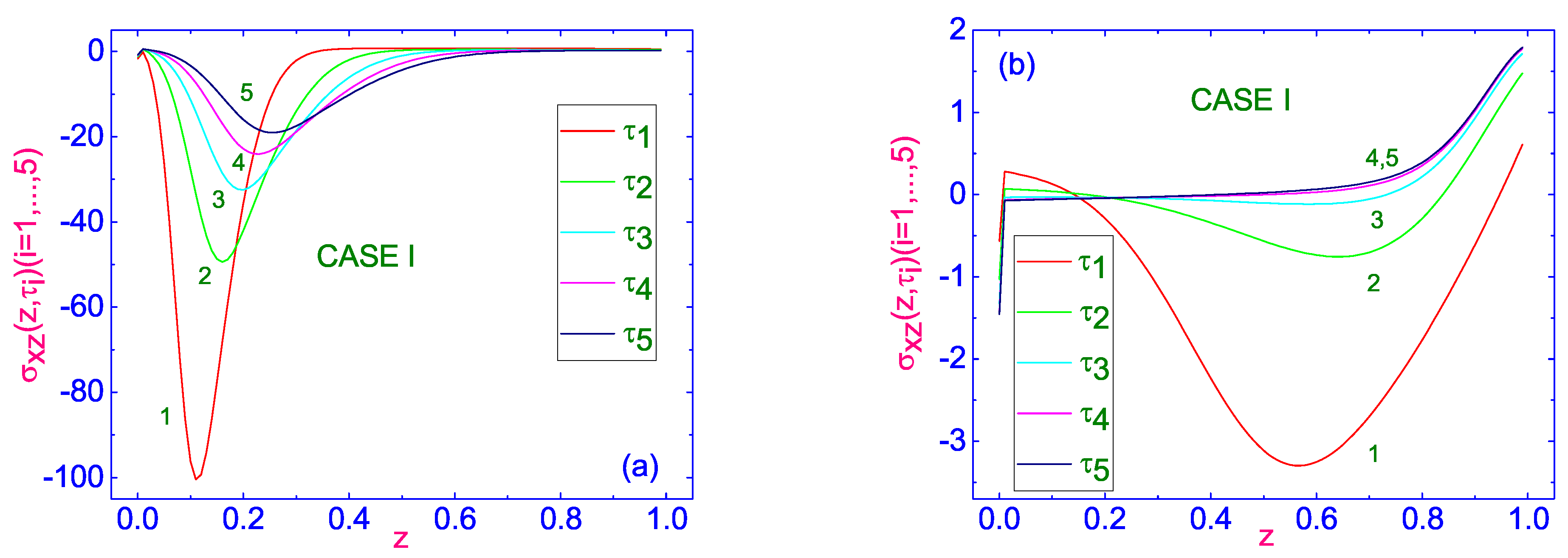
The evolution of dimensionless shear stress tensor (ST) component ${\sigma }_{\mathrm{xz}}(z,{\tau }_i)(i=1,\cdots ,5)$ as the function of the dimensionless distance z counted from the lower cooler ${\chi }_{\mathrm{z}=0}={\chi }_1$ to the upper warmer ${\chi }_{\mathrm{z}=1}={\chi }_1+\Delta \chi$ (case I) bounding surface, during the first 5 dimensionless time terms ${\tau }_i={\tau }_{0}i,(i=1,\cdots ,5)$, whose values increase from curve (1) to curve (5), is shown in Figure 5a.

Here, ${\chi }_1=0.97$, $\Delta \chi =0.0162$ and ${\tau }_0=0.01$. During the first 5 time terms ${\tau }_i={\tau }_{0}i,(i=1,\cdots ,5)$, the maximum absolute value of $|{\sigma }_{\mathrm{xz}}(z,\tau )|$ decreases rapidly with $|{\sigma }_{\mathrm{xz}}(z,{\tau }_1)|\sim 100$ to $|{\sigma }_{\mathrm{xz}}(z,{\tau }_5)|\sim 20$, by about five times less, and this maximum is located near the lower cooler bounding surface. One of the features of this relaxation is that the values of the shear ST tensor ${\sigma }_{\mathrm{xz}}(z,\tau )$ are negative during the first 5 time terms ${\tau }_i={\tau }_{0}i,(i=1,\cdots ,5)$. During the last 5 time terms, ${\tau }_i={\tau }_{0}i,(i=1,\cdots ,5)$ (see Figure 5b), where ${\tau }_0=0.1$, the value of ${\sigma }_{\mathrm{xz}}(z,{\tau }_1)$ decreases rapidly near the lower bounding surface from ${\sigma }_{\mathrm{xz}}(z\sim 0,{\tau }_1)\sim -1.5$ to ${\sigma }_{\mathrm{xz}}(z\sim 0,{\tau }_1)\sim 0.25$ with further oscillation across the thickness of the HACN channel. The equilibrium distribution of ${\sigma }_{\mathrm{xz}}(z,{\tau }_5)\equiv {\sigma }_{\mathrm{xz}}(z,{\tau }_{\mathrm{eq}})$ is characterized by a monotonous increase in ${\sigma }_{\mathrm{xz}}(z,\tau )$ from $-1.5$ on the lower bounding surface to $1.8$ on the upper hotter bounding surface.

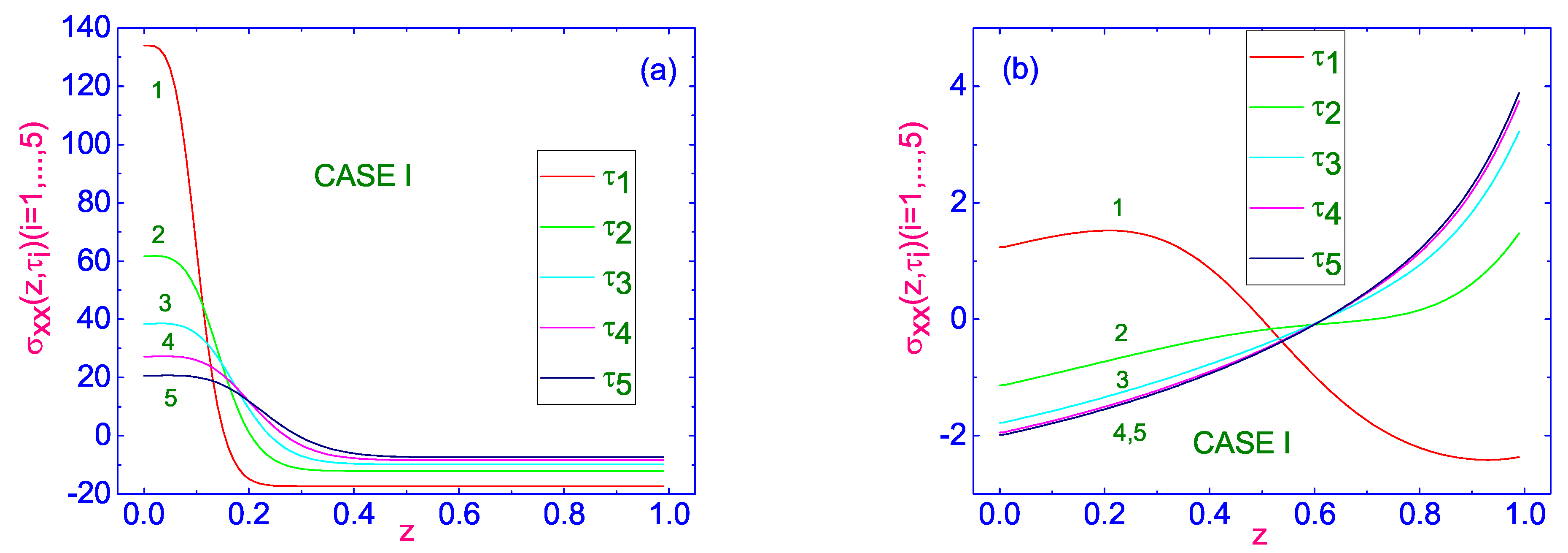
In turn, the evolution of dimensionless normal ST component ${\sigma }_{\mathrm{xx}}(z,{\tau }_i)(i=1,\cdots ,5)$ as the function of the dimensionless distance z, during the first 5 dimensionless time terms ${\tau }_i={\tau }_{0}i,(i=1,\cdots ,5)$, whose values increase from curve (1) to curve (5), is shown in Figure 6a.

As in the case of shear ST, during the first 5 time terms ${\tau }_i={\tau }_{0}i,(i=1,\cdots ,5)$, the maximum absolute value of $|{\sigma }_{\mathrm{xx}}(z,\tau )|$ decreases rapidly with $|{\sigma }_{\mathrm{xx}}(z,{\tau }_1)|\sim 135$ to $|{\sigma }_{\mathrm{xx}}(z,{\tau }_5)|\sim 20$, about more than 6 times less, and this maximum is located near the lower cooler bounding surface. One of the features of this relaxation is that the values of the normal ST tensor ${\sigma }_{\mathrm{xx}}(z,\tau )$ are negative during the first 5 time terms ${\tau }_i={\tau }_{0}i,(i=1,\cdots ,5)$, over most of the channel thickness, while in the area close to the lower restricted surface, these values are positive. During the last 5 time terms, ${\tau }_i={\tau }_{0}i,(i=1,\cdots ,5)$ (see Figure 6b), where ${\tau }_0=0.1$, the value of ${\sigma }_{\mathrm{xx}}(z,{\tau }_1)$ is characterized by a monotonous increase from the negative ${\sigma }_{\mathrm{xx}}(z\sim 0,{\tau }_1)\sim -2.0$, near the lower surface, to ${\sigma }_{\mathrm{xx}}(z\sim 1.0,{\tau }_5)\sim 4.0$, near the upper surface, respectively.

The relaxation of the rest ST components ${\sigma }_{\mathrm{zx}}\left(\tau \right)$ and ${\sigma }_{\mathrm{zz}}\left(\tau \right)$ to their equilibrium values ${\sigma }_{\mathrm{zx}}^{eq}\left(\tau \right)$ and ${\sigma }_{\mathrm{zz}}^{eq}\left(\tau \right)$, during the last 5 time terms, ${\tau }_i={\tau }_{0}i,(i=1,\cdots ,5)$, where ${\tau }_0=0.1$, and described by Equations (22) and (23), are shown in Figure 7a and Figure 7b, respectively.

Taking into account that both ST components ${\sigma }_{\mathrm{zx}}\left(\tau \right)={\mathcal{C}}_1\left(\tau \right)$ and ${\sigma }_{\mathrm{zz}}\left(\tau \right)={\mathcal{C}}_2\left(\tau \right)$ do not depend on z, they have been fixed by the boundary conditions. Both the equilibrium distributions of ${\sigma }_{\mathrm{zx}}\left({\tau }_5\right)\equiv {\sigma }_{\mathrm{zx}}\left({\tau }_{\mathrm{eq}}\right)=-1.2$ and ${\sigma }_{\mathrm{zz}}\left({\tau }_5\right)\equiv {\sigma }_{\mathrm{zz}}\left({\tau }_{\mathrm{eq}}\right)\sim -2.8$ are characterized by negative values. The above distributions of the ST components show that in the HACN channel, under the effect of the temperature gradient $\nabla \chi$, directed from cooler lower to hotter upper bounding surfaces, a complex, mainly horizontal flow is excited in the negative direction (see Figure 3a).

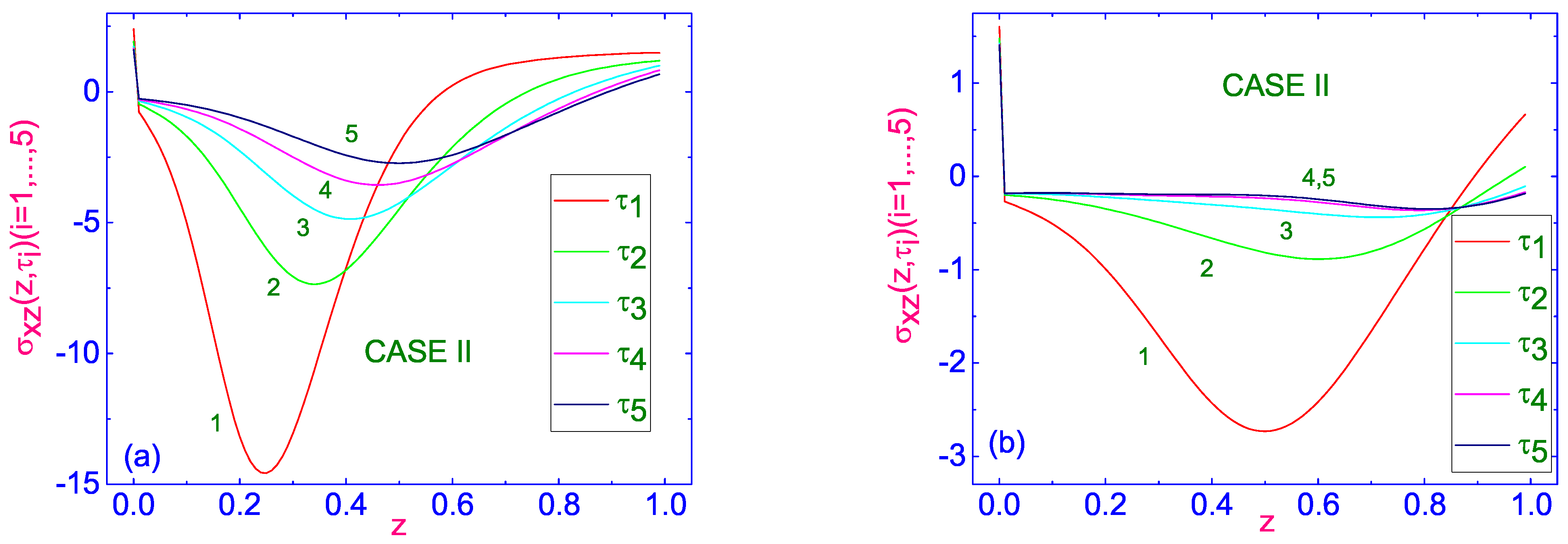
In case II, when the LC sample is heated from below with the dimensionless temperature difference $\Delta \chi =0.0162$ ($\sim 5$ K), the evolution of dimensionless shear ST component ${\sigma }_{\mathrm{xz}}(z,{\tau }_i)(i=1,\cdots ,5)$ as the function of the dimensionless distance z counted from the lower hotter ${\chi }_{\mathrm{z}=0}={\chi }_1+\Delta \chi$ to the upper cooler ${\chi }_{\mathrm{z}=1}={\chi }_1$ bounding surface, during the first 5 dimensionless time terms ${\tau }_i={\tau }_{0}i,(i=1,\cdots ,5)$, whose values increase from curve (1) to curve (5), is shown in Figure 8a.

Here, ${\chi }_1=0.97$, $\Delta \chi =0.0162$ and ${\tau }_0=0.01$. During the first 5 time terms ${\tau }_i={\tau }_{0}i,(i=1,\cdots ,5)$, the maximum absolute value of $|{\sigma }_{\mathrm{xz}}(z,\tau )|$ decreases rapidly with $|{\sigma }_{\mathrm{xz}}(z,{\tau }_1)|\sim 15$ to $|{\sigma }_{\mathrm{xz}}(z,{\tau }_5)|\sim 2.0$, by about 7 times less, and this maximum is located near the center of the HACN channel. One of the features of this relaxation is that the values of shear ST tensor ${\sigma }_{\mathrm{xz}}(z,\tau )$ are negative during the first 5 time terms ${\tau }_i={\tau }_{0}i,(i=1,\cdots ,5)$. During the last 5 time terms, ${\tau }_i={\tau }_{0}i,(i=1,\cdots ,5)$ (see Figure 8b), where ${\tau }_0=0.1$, the value of ${\sigma }_{\mathrm{xz}}(z,{\tau }_1)$ decreases rapidly near the lower bounding surface from ${\sigma }_{\mathrm{xz}}(z\sim 0,{\tau }_1)\sim 1.2$ to ${\sigma }_{\mathrm{xz}}(z\sim 0,{\tau }_1)\sim -0.25$, with a further decrease to the value ${\sigma }_{\mathrm{xz}}(z\sim 0.5,{\tau }_1)\sim -2.7$, and a further gradual increase up to $0.8$, near the upper bounding surface. Equilibrium distribution of ${\sigma }_{\mathrm{xz}}(z,{\tau }_5)\equiv {\sigma }_{\mathrm{xz}}(z,{\tau }_{\mathrm{eq}})$ is characterized by an almost constant small negative value across the LC channel.

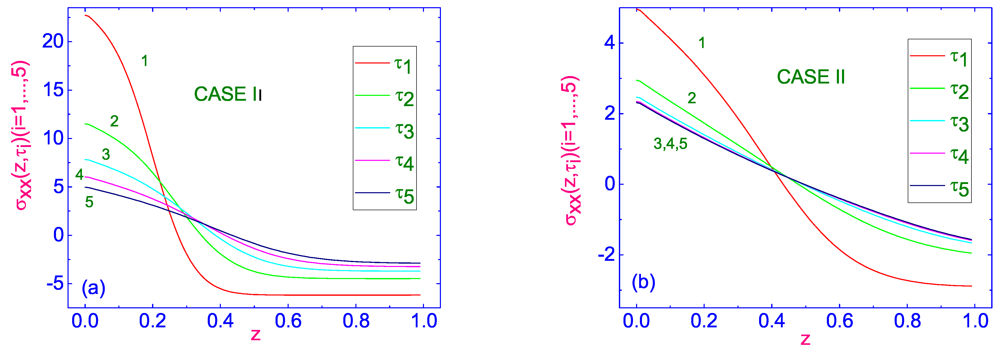
In turn, the evolution of dimensionless normal ST component ${\sigma }_{\mathrm{xx}}(z,{\tau }_i)(i=1,\cdots ,5)$ as the function of the dimensionless distance z, during the first 5 time terms ${\tau }_i={\tau }_{0}i,(i=1,\cdots ,5)$, whose values increase from curve (1) to curve (5), is shown in Figure 9a.

As in case I, during the first 5 time terms ${\tau }_i={\tau }_{0}i,(i=1,\cdots ,5)$, the maximum absolute value of $|{\sigma }_{\mathrm{xx}}(z,\tau )|$ decreases rapidly with $|{\sigma }_{\mathrm{xx}}(z,{\tau }_1)|\sim 23$ to $|{\sigma }_{\mathrm{xx}}(z,{\tau }_5)|\sim 5$, by about more than 4 times less, and this maximum is located near the lower hotter bounding surface. One of the features of this relaxation is that the values of the normal ST component ${\sigma }_{\mathrm{xx}}(z,\tau )$ are positive during the first 5 time terms ${\tau }_i={\tau }_{0}i,(i=1,\cdots ,5)$, only near the lower hotter bounding surface, while in the rest area of the LC channel, these values are negative. During the last 5 time terms, ${\tau }_i={\tau }_{0}i,(i=1,\cdots ,5)$ (see Figure 9b), where ${\tau }_0=0.1$, the value of ${\sigma }_{\mathrm{xx}}(z,{\tau }_5)$ is characterized by a gradual decrease from the positive ${\sigma }_{\mathrm{xx}}(z\sim 0,{\tau }_5)\sim 2.3$, near the lower surface, to ${\sigma }_{\mathrm{xx}}(z\sim 1.0,{\tau }_5)\sim -1.6$, near the upper surface, respectively.

The relaxation of the rest ST components ${\sigma }_{\mathrm{zx}}\left(\tau \right)$ and ${\sigma }_{\mathrm{zz}}\left(\tau \right)$ to their equilibrium values ${\sigma }_{\mathrm{zx}}^{eq}\left(\tau \right)$ and ${\sigma }_{\mathrm{zz}}^{eq}\left(\tau \right)$, during the last 5 time terms, ${\tau }_i={\tau }_{0}i,(i=1,\cdots ,5)$, where ${\tau }_0=0.1$, and described by Equations (22) and (23), are shown in Figure 10a and Figure 10b, respectively.

As in case I, in case II, both ST components ${\sigma }_{\mathrm{zx}}\left(\tau \right)={\mathcal{C}}_1\left(\tau \right)$ and ${\sigma }_{\mathrm{zz}}\left(\tau \right)={\mathcal{C}}_2\left(\tau \right)$ do not depend on z, and they have been fixed by the boundary conditions. Both the equilibrium distributions of ${\sigma }_{\mathrm{zx}}\left({\tau }_5\right)\equiv {\sigma }_{\mathrm{zx}}\left({\tau }_{\mathrm{eq}}\right)=0.773$ and ${\sigma }_{\mathrm{zz}}\left({\tau }_5\right)\equiv {\sigma }_{\mathrm{zz}}\left({\tau }_{\mathrm{eq}}\right)\sim -2.45$ are characterized by positive and negative values, respectively. The above distributions of the ST components show that in the HACN channel, under the effect of the temperature gradient $\nabla \chi$, directed from cooler upper to hotter lower bounding surfaces, a complex, mainly horizontal flow is excited in the positive direction (see Figure 3b).

It should be noted that in cases I and II, hydrodynamic flows of different magnitudes and directions are formed in the LC channel under the effect of the same temperature gradient $\nabla \chi$ but directed in the opposite directions.

4. Conclusions

In summary, we have investigated the relaxation of director $\widehat{\mathbf{n}}(\mathbf{r},t)$, velocity $\mathbf{v}(\mathbf{r},t)$, and stress tensor components ${\sigma }_{\mathrm{ij}}(z,t)(\mathrm{i},\mathrm{j}=\mathrm{x},\mathrm{z})$ in the HACN channel to their equilibrium values, under the influence of the temperature gradient directed normal to the bounding surfaces. Our calculations, based upon the classical Leslie–Ericksen theory, show that the hybrid-aligned compressible nematic material under the effect of the temperature gradient $\nabla T$, directed from the lower cooler to upper hotter bounding surfaces, settles down to a stationary flow regime with the horizontal u and vertical w components of velocity, which sufficiently differ from these components under the effect of the same $\nabla T$ but directed from lower hotter to upper cooler bounding surfaces.

Note that in the case of a hybrid-aligned incompressible nematic (HAIN) channel, where due to the incompressibility condition $\nabla ·\mathbf{v}=0$ and the boundary no-slip condition for the velocity field there is only one nonzero component of the vector $\mathbf{v}$, $viz.$, $\mathbf{v}=v_x\widehat{\mathbf{i}}=u\widehat{\mathbf{i}}$, the character of the stationary distribution of the horizontal component of velocity $u_{\mathrm{eq}}\left(z\right)\left(\mathrm{HAIN}\right)$ differs sufficiently from the same stationary distribution of the horizontal component of velocity $u_{\mathrm{eq}}\left(z\right)\left(\mathrm{HACN}\right)$ for a hybrid-aligned compressible nematic channel. This difference is due to the different behavior of $\nabla \widehat{\mathbf{n}}$ and $\nabla \chi$ across the LC sample.

We believe that the present study may shed some light on the problem of the reorientation process in a compressible nematic channel under the influence of a vertical temperature gradient. We also believe that this paper shows not only some useful routes for estimating relaxation times but also for analyzing the remaining problems associated with an LC^′ device’s stability, efficiency, and lifetime.