Article

Unraveling the Determinant Mechanisms in Flow-Mediated Crystal Growth and Phase Behaviors

1
Department of Chemical and Biomedical Engineering, Florida A&M University-Florida State University College of Engineering, 2525 Pottsdamer St, Tallahassee, FL 32310, USA
2
Sandia National Laboratories, 1515 Eubank Blvd SE, Albuquerque, NM 87123, USA
*
Author to whom correspondence should be addressed.
Crystals 2025, 15(2), 157; https://doi.org/10.3390/cryst15020157
Submission received: 28 December 2024 / Revised: 22 January 2025 / Accepted: 28 January 2025 / Published: 4 February 2025
(This article belongs to the Special Issue Crystallization Process and Simulation Calculation, Third Edition)

Abstract

:
To uncover the critical mechanisms responsible for mesoscopic level development during flow-mediated crystal growth, we develop a semi-two-way hydrodynamic coupled structural phase-field crystal formalism (HXPFC-s2). The new formalism, inspired by previous attempts at coupling hydrodynamic and phase-field crystal (PFC) equations, allows for studying mesoscopic flow-mediated crystallization at diffusive timescales pertinent to industrial applications. Unlike previous efforts, the devised coupling to the structural PFC (XPFC) equations allows generalization to more complex crystal structures through explicit parameterization of the direct correlation function (DCF). Utilizing the HXPFC-s2 formalism, we seek to uncover the determinant physical mechanisms in crystallization under simple shear flows by comparing temperature-driven crystallization to flow-mediated crystallization under varying flow-strengths. Parallels and deviations of under-cooling and flow-strength effects on crystal growth are drawn using the crystal cluster-size and system ordering time evolutions. In doing so, we identify scaling behaviors with a Peclet-like number, Pe , a critical Peclet-like number, Pe * , and flow-field-crystal plane-dependent interactions. Our findings may be relevant for controlling crystal growth and phase behaviors in flow applications.

1. Introduction

With the ever-growing desire for clean energy technology, perovskite-based solar cells (PSCs) have emerged as a potential solution. With their power conversion efficiencies (PCEs) reaching approximately 25%, they are now able to compete with leading solar cell technologies such as semiconductors [1]. Unfortunately, the main challenge with the implementation of PSCs on a global scale is due to the lack of cost-effective, scalable manufacturing techniques to handle the unique molecular-level crystallization defects and instabilities. These defects have been observed in most common solution-based techniques, such as laboratory-scale spin coating, and have been shown to decrease efficiency [1,2,3,4]. Hence, moving clean technology out of the lab and into markets requires tunable manufacturing techniques that are adaptable to the defect-prone processing of PSCs. The most successful and recent attempt at up-scaling PSC thin-film manufacturing utilized roll-to-roll manufacturing of slot-die coated perovskite ink (solution) [4]. Other scalable solution-based methods include blade coating, inkjet printing, and spray coating [2,3]. The most commonly suggested techniques for aiding in scalable and high-performance PSC thin-film solution processing have typically focused on solvent and composition engineering [1,3]. However, there is little mention of the impact of hydrodynamic forces during solution processing. Guo et al. showed that the perovskite solution is subject to both shear and inertial forces during processing by macroscopic numerical modeling of slot-die coating of PSC thin films [5]. In addition, evaporation using an air knife over the wet-film surfaces during slot-die coating has been reported to be highly effective for production [3,4]. There is a need for a more in-depth understanding of how best to control grain growth kinetics during PSC thin-film growth [2]. We believe that hydrodynamic interactions during crystallization could be another optimization dimension not commonly considered in the scale-up of PSC thin-film technologies. Furthermore, in other solution crystallization processes, flow is shown to be a process optimization variable in addition to supersaturation and temperature [6,7,8]. Hence, we seek to address the knowledge gap by utilizing a simplified particle-in-fluid model coupling the Structural Phase Field Crystal (XPFC) formalism to the Navier–Stokes equations in a semi-two-way manner that we term semi-two-way hydrodynamic coupled structural phase-field crystal (HXPFC-s2).
The Phase Field Crystal (PFC) method [9,10] is a numerical technique deeply rooted in statistical mechanics and the traditional theories of freezing [11,12]. First introduced in 2002 by Elder et al. [9], PFC models have had success in probing crystalline materials such as in grain boundary migration [13], lattice defects [14,15], and nucleation and crystal growth [16]. In addition, attempts have been made to study the influence of flow dynamics on crystallization using the PFC family of equations [17,18,19,20]. The original PFC method has a direct link to DDFT, originally derived from the Langevin equation of motion using stochastic calculus from Dean [21] and elegantly expanded by Marconi and Tarazona [22]. Their works were directly translated to the PFC formalism in references [17,18,23]. In summary, by evolving the equilibrium free energy functional for the density, F [ ρ ( r ) ] , or order-parameter, F [ ψ ( r ) ] , fields (DDFT or PFC, respectively), the system not only follows dynamics described by the Langevin equation of motion for Brownian particles, but also captures the particle interactions,
ρ t = ρ ( r , t ) δ F [ ρ ( r ) ] δ ρ ,
where ρ ( r ) is the number density, t is time, r is the position vector, and F [ ρ ( r ) ] is the free-energy functional.
Elder et al. [9,10,12] further extended the approximations from the DDFT equations by using a Taylor expansion of the natural-log in the ideal (translational) contribution to the free energy functional,
F I D [ ρ ( r ) ] = k B T d r ρ ( r ) [ ln ( ρ ( r ) ) 1 ] ,
and expanding the Direct Correlation Function (DCF),
C ( 2 ) ( r , r ) = β δ 2 F δ ρ ( r ) δ ρ ( r ) ,
in Fourier space resulting in the familiar Swift–Hohenberg form of the PFC free energy functional; see, for example, [12,24], where k B is the Boltzmann constant, T is temperature, and β = 1 k B T . In 2011, Greenwood and Provatas [25,26] introduced a form of the free energy functional called the Structural Phase Field Crystal (XPFC) in which, rather than expanding the DCF inside the excess free energy functional,
F E X [ ρ ( r ) ] = k B T 2 d r d r Δ ρ ( r ) C ( 2 ) ( | r r | ) Δ ρ ( r ) ,
in Fourier space, the DCF was approximated by utilizing the most energy-dominant crystal planes. By employing an ansatz for the DCF, Greenwood and Provatas enabled the ability to model more complex structures, include multi-body interactions through higher-order correlation functions, and potentially parameterize much more easily. Additionally, in 2011, Praetorious and Voigt first attempted the Navier–Stokes coupled PFC equations to model colloidal particles in solvent using a diffuse domain approach [17]. In 2015, Praetorious and Voigt much more rigorously expanded the 2011 model to not only capture colloidal particles in solvent, but also pave the way for analyzing crystal growth in flow with PFC methods [18]. To date, most of the works utilizing their PFC-Navier–Stokes model seek to gain insight into the numerical analysis [27] or novel numerical methods [28,29,30], rather than understanding the physical role of fluid flow on crystallization. By utilizing previous works from the DDFT line of thought [21,22,23,31], the original PFC formalism was coupled with the Navier-Stokes equations to study flow effects [17,18,20]. In this work, we extend the previous attempts by coupling Navier–Stokes equations to the XPFC equations in an attempt to make the model more flexible without compromising the determinant flow physics. Specifically, the model treats the momentum coupling exclusively through a forcing term capturing the chemical potential gradient while neglecting viscous coupling. Using the semi-two-way coupled model, which we call HXPFC-s2, the effects of flow hydrodynamics during post-critical nucleus crystal growth are studied to help gain mechanistic insights into considering flow for the optimization of large-scale PSC thin-film production.
The paper is organized as follows. In Section 2, we cover the derivation of the HXPFC-s2 formalism, highlighting the physical considerations of the process. Full derivation details are provided in Appendix A. In Section 3, we compare temperature-driven and flow-mediated crystallization using the cluster-size and ordering to understand mechanistically how flow impacts crystal growth. In Section 4 and Section 5, we discuss and summarize the findings, respectively.

2. Materials and Methods

2.1. HXPFC-s2 Formalism

Building on the works of [17,21,22,23,26,32,33], we present the HXPFC-s2 formalism, describing crystallization in fluid flow, which includes the momentum (5a), the continuity (5b), the advected XPFC (order-parameter) (6), the chemical potential, μ , Equation (7a), and the Fourier-space DCF, C ^ ( | k | ) , equations. Parameters are defined in Table 1.
u t + · ( uu ) = P ¯ + · ν u + ( u ) T + k B T m ψ δ F [ ψ ( r ) ] δ ψ
· u = 0
ψ t + u · ψ = M 2 δ F [ ψ ( r ) ] δ ψ + 2 M · ξ ( t )
μ ( r ) = δ F [ ψ ( r ) ] δ ψ = ψ ( r ) ψ ( r ) 2 2 + ψ ( r ) 3 3 d r C ( 2 ) ( | r r | ) ψ ( r )
C ^ ( | k | ) = i exp σ 2 k i 2 2 ρ i β i exp ( | k | k i ) 2 2 α i 2
For more details on the full derivation of Equations (5a)–(7a), see Appendix A.1, for the form of the free energy functional used to obtain Equation (7a), Appendix A.2 for the origin of Equation (6), and Appendix A.3 for the momentum coupling in Equation (5a). Also, see references [17,21,22,23,24,26,32,33,35,36]. We briefly highlight the important aspects to understanding crystallization through the lens of the HXPFC-s2 equations. Additionally, the equations are explained in order of information flow, as the Free Energy Functional, Equation (7a), and DCF, Equation (7b), inform the advected XPFC, Equation (6), which couples with the Navier–Stokes.

2.1.1. Free Energy Functional and Advected XPFC Equation

The form of the free energy functional to obtain Equation (7a) originates from changing the free energy into functional form by utilizing N = d r ρ ( r ) , and the canonical partition function [36]. The functional derivative of the free energy functional density form,
δ F [ ρ ( r ) ] δ ρ = k B T ln ( ρ ( r ) ) + β U e x t ( r ) d r C ( 2 ) ( | r r | ) Δ ρ ( r ) ,
including an external potential field, U e x t , can be easily converted into the PFC form.
The connection to the physical system contained in the excess free energy functional is not fully realized until the origin of advected XPFC Equation (6), via DDFT, Equation (1), is developed. Fundamentally, the system described by Equations (1) and (6) corresponds to a collection of Brownian particles whose motion is characterized by the Langevin equations of motion in the over-damped limit (damping coefficient, ω m 1 ) in the presence of bulk fluid flow [17,21,22,23,32,37]. The Langevin equations read
d r i d t = v i ,
m i d v i d t = ω m i ( v i u ( r i , t ) ) i = 1 N U n b ( | r i r j | ) + 2 ω m i k B T ξ i ( t ) ,
where ω is the damping frequency, v i is the velocity of particle i, u i is the fluid velocity at particle i, and U n b ( | r i r j | ) is the non-bonded pair-wise intermolecular potential.
In the over-damped limit, the acceleration term in Equation (9b) becomes negligible, and the particle velocity is governed by the bulk fluid flow, particle–particle interactions, and thermal motion. After rearranging into a stochastic integral equation form with respect to the particle positions, utilization of Ito’s Lemma, and integration by parts, Equation (9b) becomes [17,21,22,23,35],
ρ ( r ) t + · ( ρ ( r ) u ( r ) ) = 1 ω m · k B T ρ ( r ) + ρ ( r ) d r U n b ( | r r | ) ρ ( r ) .
Note that the noise term was left out of (10) for simplicity. Upon comparing Equations (8) and (10), it can be seen that [18,21,22,23]
k B T ρ ( r ) = k B T ρ ( r ) ln ( ρ ( r ) ) = ρ ( r ) δ F I D [ ρ ( r ) ] δ ρ ,
u ( r ) = 1 ω m U e x t = 1 ω m δ F E X T [ ρ ( r ) ] δ ρ .
However, determining how the DCF, C ( 2 ) ( | r r | ) , as a result of the Ramakrishnan and Yussouff approximation [11], is physically related to the non-bonded intermolecular potential, U n b ( | r r | ) , may not be immediately obvious. The immediate solution is simply noticing that U n b ( | r r | ) C ( 2 ) ( | r r | ) and from integral equation theory closures, there are a few solutions to elucidate the meaning, with similar explanations. Because of their success in recovering certain fluid thermodynamic properties, the two closures that best directly connect the intermolecular potential and the DCF here are the hypernetted chain (HNC) and mean spherical approximation (MSA) closures [36,38,39]. However, the HNC only asymptotically approaches the MSA at large particle separations, ( | r r | ) , whereas the MSA mainly applies to hard sphere fluids, U n b ( | r r | < d p ) = , where d p is the particle diameter (or inter-molecular potentials that approximate hard-spheres). Hence, at large particle separations in the HNC approximation, or more aptly, the MSA, it is found that U n b ( | r r | ) = k B T C ( 2 ) ( | r r | ) [36,39]. Additionally, te Vrugt et al. [40] showed that a random phase approximation (RPA) could be used to make the connection between the intermolecular potential and DCF. Hansen and Macdonald [36] have shown that the RPA, along with the condition that C ( 2 ) ( | r r | < d p ) = 0 , is a more exact statement of the MSA for hard-spheres, but is similar in interpretation. If the density is then expanded about a reference density, ρ ( r ) = ρ r e f + Δ ρ ( r ) ,
d r U n b ( | r r | ) ρ ( r ) k B T d r C ( 2 ) ( | r r | ) Δ ρ ( r ) = F E X [ ρ ( r ) ] ρ ,
where the reference density vanishes because of the functional derivative and gradient operator [40]. Equation (13) is the form directly translatable into the XPFC chemical potential, Equation (7a). Alternatively, an adiabatic approximation [41] can be made to link the intermolecular potential and DCF. By approximating the time-evolution through a series of equilibrium states, a ‘deterministic’ DDFT results [22,40].
After inserting Equations (11)–(13) into Equation (10), changing variables yields Equation (6). The interfacial mobility becomes M = k B T ω m , effectively a diffusion coefficient due to the phase change. As a result of the MSA closure, Equations (6) and (10) describe the evolution of particle density fields whose interactions are governed by hard sphere intermolecular potentials plus an attractive tail [36]. The MSA has had great success in modeling simple ionic solutions [38,42]. Additionally, hard rods were modeled semi-successfully in the original DDFT formalism [22] and others have used hard sphere fluids to model crystallization in a drying film [43]. For a full review of DDFT method successes, see [40].

2.1.2. Navier–Stokes Momentum Coupling

An immersed boundary approach was taken when coupling the advected XPFC, Equation (6), to the Navier–Stokes equations [18,44] in a semi-two-way coupled manner [37]. However, the forcing term to account for the presence of the particles in the fluid was summed over the particle positions, rather than boundary nodes in immersed boundary methods [44]. The forcing term in Equation (5a) becomes
f ( r ) = d r i F ( r i ) δ ( | r r i | ) .
We take the body forcing term at particle i [18,37] as
F i = ω m i ( v i u ( r i , t ) ) .
By utilizing the force balance in Equation (9b), Equation (15) must be balanced by the thermal noise and the gradient in intermolecular forces, leading to
F i = j = 1 N U n b ( | r i r j | ) + 2 ω m i k B T ξ i ( t ) .
Since ρ ( r ) = i ρ i ( r ) = i δ ( | r r i | ) , Equation (14) is approximated as
f ( r ) = d r i F ( r i ) δ ( | r r i | ) i F i ( r i ) ρ i ( r ) .
After taking the same particle-to-grid transformation using Ito’s lemma that led to Equation (10), one arrives at the forcing term, in terms of number density, that is included in Equation (5a):
f ( r ) = ρ ( r ) δ F [ ρ ( r ) ] δ ρ .
We note that a noise term that arose as a consequence of the transformation was excluded from Equation (18).

2.2. HXPFC-s2 Dimensionless Form

In the remainder of the paper, the dimensionless form of Equations (5a)–(6) will be utilized. In doing so, we focus on studying the critical physics without restricting ourselves to a specific system. Equations (7a) and (7b) are naturally in dimensionless form. When non-dimensionalizing Equations (5a)–(6), we use both the convective and diffusive timescales to extract dimensionless groups. The critical dimensionless groups are defined in Section 2.3, Table 2. However, in the simulations in Section 3, we only utilize the convective timescale form,
u τ + · ( u u ) = Eu P + 1 Re · ν u + ( u ) T + Eu ψ δ F [ ψ ( r ) ] δ ψ
· u = 0
ψ τ + u · ψ = 1 Pe 2 δ F [ ψ ( r ) ] δ ψ + 2 M u 0 · ξ ( t ) .
For more information, see Appendix B.1 and Appendix B.2 for obtaining the convective and diffusive timescale forms, respectively. In addition, Equation (19a) was left general by expanding about a reference viscosity ν ( r ) = ν 0 Δ ν ( r ) ν 0 + 1 , where ν 0 is the reference liquid viscosity [18,45]. However, in the simulations in Section 3, the viscosity was taken as a constant ν = ν 0 , hence the semi-two-way coupling and the name HXPFC-s2. As the full-two-way coupling is not needed to study the dynamics of the Peclet-like number, Pe on crystal growth, we elect to focus on semi-two-way coupling exclusively and keep the full-two-way coupling implementation as future work. Simplicity is achieved by neglecting the particle viscosity difference in Equation (19a). However, only treating the momentum coupling through the forcing term in Equation (19a) leads to large contributions from the Euler-like number, Eu , to the flow-field. Hence, to fully realize the dynamics of Re and Eu , the full-two-way coupling should be implemented via the viscosity; see Section 2.3, Equation (22). Therefore, the flow-mediated crystallization physics are governed, most realistically, by Pe in the HXPFC-s2 model.

2.3. Significant Dimensionless Numbers

The formalism-specific dimensionless numbers we found most impacted are listed, and their physical meanings are listed in Table 2.
Note, the Reynolds (Re) and Euler (Eu) numbers retain their traditional definitions from fluid mechanics. The Schmidt-like number, Sc , is missing explicitly from Equations (19a)–(20), but it may be obtained by dividing Pe by Re or naturally normalizing by the diffusive timescale as in Appendix B.2. The Peclet-like number, Pe , directly impacts the order-parameter by acting as an effective interfacial diffusion coefficient in Equation (6) and also impacts the particle–particle interactions in (9b) and (10). Thus, we prioritize analyzing the effects of Pe on crystal growth in this work.
The effects of Eu may not be as obvious, but Eu clearly affects the particle–fluid interactions by modulating the forcing term in Equation (19a). The energy scaling, k B T , in Eu resulted from the pre-factor in the free energy functional (8), which was convenient in defining Eu , but gives little aid in deciphering the physical meaning. The traditional fluid mechanic definition of Eu is the ratio of the pressure driving force (in pressure-driven fluid flow) to inertial forces, indicating Eu must contain similar physics. Hence, modifying the definition of Eu with the chemical potential difference, Δ μ S L = Δ G S L , between the solid and liquid phases, which is the driving force of crystallization, a new meaning for Eu emerges as the ratio of crystallization driving force to inertial forces. However, to obtain Δ μ S L = Δ G S L , insight can be gained from classical nucleation theory (CNT),
Δ G ( r ) = 4 3 π r 3 Δ G S L + 4 π r 2 σ S L ,
where Δ G S L is the solid–liquid Gibbs free energy (chemical potential) difference, also known as the crystallization driving force, and σ S L is the solid–liquid interfacial energy. Therefore, if one phenomenologically normalizes the chemical potential with the Δ μ S L , obtained from the critical (maximum) Gibbs free energy, Δ G * , from CNT (see Figure 1 and Equation (21)), replacing k B T with Δ μ S L , the Eu ratio now represents the ratio of crystallization driving force to inertial driving forces, directly analogous to Eu. Additionally, because Δ G * k B T , the idea that Eu represents the ratio of driving forces is not completely unrealistic (for example, using the TIP4P/2005 water model, it was found that with a 29.5   K under-cooling, Δ G * 77 k B T [46]). Hence, according to Eu , the greater the driving force of crystallization (solubility limit, under-cooling, etc.), the greater the disruption of the flow-field due to crystallization.
De is another parameter that elucidates the ratio of different timescales and is a result of analyzing Equation (19a) in the Stokes regime in the absence of a pressure gradient,
· ν u + ( u ) T = Eu Re ψ δ F [ ψ ( r ) ] δ ψ .
The result of multiplying Re by Eu yields a parameter of the form De Sc , which contains information on the ratio of timescales in the system. Additionally, it elucidates the intricate relationship between the individual particle and the growing crystal geometries, fluid properties, interfacial properties, and the strength of fluid flow. Hence, the Re and Eu parameters lead to coupled dynamics, and the effects of Eu become dependent on the value of Re. This relationship is the link between the solvent/melt properties through Re, the crystallization properties through Eu , and advective flow.

2.4. Numerical Methods

We utilize the dimensionless form of the HXPFC-s2 only to study the effects of the dimensionless parameters on flow-mediated crystallization. Additionally, a staggered-grid projection scheme [47] is used, instead of the usual pseudo-spectral technique, to include wall-bounded flows for isolating and studying the effects of shear-flow observed in scalable thin-film technologies. Specifically, we study the effects of simple shear flow on a growing crystal seed in two dimensions, as shown in Figure 2. The full details of the numerical scheme are discussed in reference [33]. However, we include the most critical aspects.
In the HXPFC-s2 formalism, Equation (7a) is first solved by mirroring the domain once in the non-periodic direction, extending once in the periodic direction, and then solving a four-times-larger grid using the Fast-Fourier Transform (FFT) [33,48]. Once the chemical potential was obtained, Equation (6) was solved using an explicit second-order centered difference on the cell vertices of the staggered grid. The method captures Neumann boundary conditions with respect to the order-parameter, ψ . When excluding the boundary effects (stopping the simulation before it interacts with the wall), it was shown to retain good accuracy when comparing equilibrium properties to pseudo-spectral methods [33]. Furthermore, velocities were solved on the cell edges and the pressure in the cell centers of a standard staggered grid [47]. The pressure Poisson equation was solved using a Gauss–Siedel iterative method [49], which had a good performance, even with the small error tolerances, ϵ < 1 × 10 7 , used. Time derivatives were discretized using a forward-Euler method using time-steps as follows: Pe = 0 , Δ τ D = 1 × 10 7 , Pe = 5 , Δ τ D = 5 × 10 7 , and Pe > 5 , Δ τ D = 1 × 10 6 . For choice of grid spacing, see [34].

2.5. Simulation Setup

The 2-D simulation box, including boundary conditions and domain size used in Section 3, is shown in Figure 2a.
Simple shear flow was elected over Poiseuille flow to isolate the effects of shear during crystal growth. Although, in certain coating flow applications, like slot-die coating, pressure-driven flow is present, it was shown that the coating solution experiences high shear stresses; see [5,50]. Furthermore, Praetorious and Voigt showed that Poiseuille flow can disturb the growth front of the growing crystal [18]. Hence, wall-driven flows were instead used to evenly exaggerate the effects of shear on the growing crystal. In the shear flow cases, Re = 100 , Eu = 1 , Eu = 1 , and 0 Pe 100 . The choice of Re came from low-Re laminar flows being observed in PSC film coating [5]. However, Re = 100 is higher than those reported [5], but the effects are negligible because the full two-way coupling is neglected. The Pe range is critical because it is the dominating parameter for crystal growth in HXPFC-s2. The values 0 Pe 100 correspond well to those observed experimentally in the flow alignment of rodlike particles, 0.1 Pe 10 [51]. However, it is expected that the rodlike colloidal particles will be more sensitive to flow than the quasi-spherical particle cluster.
The 2-D triangular crystal phase was studied using parameters in Table 3, which were originally reported in [34].
Initially, a seven-particle quasi-spherical seed was placed in the middle of the domain. The seed was formed by modulating the initial one-mode triangular density field approximation [12,26,34], Equation (23), by a Gaussian centered at the middle particle.
ψ t r i = A 1 2 cos 2 π x a t r i + cos π x a t r i cos 3 π y a t r i + ψ 0 ,
where A is an amplitude that is solved by energy minimization [25,34].
In setting up the box dimensions as in Figure 2a, the particle diameter is now approximately d p a r t i c l e a t r i before non-dimensionalization. After, the seed was grown to completion using the non-advected version of Equation (6), and the fully grown crystal was modulated again using a Gaussian centered at the middle particle, inspired by the procedure outlined in [29]. During the simulations, the growth velocities were analyzed by monitoring the evolution of the order-parameter, ψ , in the direction of the primary crystal planes, as shown in Figure 2b. At high Pe , the local order rearranges and tracking the plane-specific growth becomes challenging. Hence, the plane-specific growth rates are reported before the hexagonal structural decay prevents plane-specific tracking. Approximate particle positions were extracted by utilizing a modified algorithm mentioned in [33] by making use of [52]. The density field was thresholded at ψ = 0.8 and candidate particle positions were selected where the grid points (line intersections) intersected the highest part of the order-parameter field; see Figure 2c.

3. Results

The growth rate for a spherical, post-critical nucleus, originally derived from CNT in Kelton and Greer [53,54,55], is presented:
d r d t = 16 D λ 2 3 V ¯ 4 π ( 1 / 3 ) sinh V ¯ 2 k B T Δ G S L + 2 σ S L r .
where V ¯ is the atomic volume, D is the interface diffusivity, λ is the molecular jump distance.
Because of the equation’s simplicity, it can be easily linearized and fit to growth rate data. Hence, we utilize the dimensionless PFC form to fit, interpret, and connect the toy model results to physical values:
v = 16 3 4 π ( 1 / 3 ) sinh 1 2 Δ G S L + σ S L r ,
where V ¯ = 1 ρ r e f , Δ G S L = Δ G S L ρ r e f k B T , σ S L = σ ρ r e f k B T , and v is the dimensionless radial growth rate. The full derivation is given in Appendix C.
Equation (25) and the no-flow HXPFC-s2 equations at σ = 0.12 and ψ 0 = 0.06 were used to generate Figure 1. The initial seven-particle crystal seed radius, r ( 0 ) 0.012 , is well above r * and the 1.5 r * requirement for accuracy when utilizing Equations (24) and (25) [54,55].
To systematically understand how shear flow mechanistically impacts crystal growth, the temperature is first studied to obtain a relatable and reliable benchmark. When studying the temperature, σ , by increasing the under-cooling, we can see if shear affects growth similarly to temperature or if another mechanism is prevalent. Therefore, we first present the impact of σ and then compare to the effects of Pe on crystal growth.

3.1. Effective Temperature-Dependent Crystal Growth

The equilibrium phase diagram and parameters used can be found in [34] or in Table 3. For clarity, we scale, τ ¯ D = 1 × 10 5 τ D . Furthermore, t and τ D can be used interchangeably here since the PFC time scale is the base time scale and τ D = t / t D with t D was set to 1. To aid in visualizing the quantitative results, the qualitative time evolution of two crystals seeds at different effective temperatures is shown in Figure 3 and Figure 4. The initial seeds are not shown because all simulations begin with the same seven particle seeds shown in Figure 2. Particle colors are as follows: σ = 0.12 is navy, σ = 0.11 is sky-blue, σ = 0.1 is pink, and σ = 0.09 is purple.
Figure 3 shows that as the triangular phase evolves from the seven-particle seed when σ = 0.12 , the particles prefer a spherical morphology and triangular structure. However, when σ = 0.09 , the system begins to change phases as it evolves in time, as shown in Figure 4. The phase change is expected because the degree of under-cooling places the meta-stable liquid in approximately the coexistence region, from the boundary lines in the σ ψ 0 equilibrium phase diagram shown in [34].
Utilizing the method listed in Section 2.5, particle positions were obtained to calculate the number of particles in the crystal as a function of time. Furthermore, the crystal plane-specific growth velocities were obtained and utilized for fitting. The full 2-D results obtained were translated into particle radius using Equation (26):
r ( t ) = 12 ( 1 / 4 ) λ s f r p a r t i c l e π 1 N ( t ) ( 1 / 2 ) ,
where λ s f 1.75 is the scaling factor, and r p a r t i c l e 0.0039 is the particle radius. Equation (26) was derived from the packing fraction of hexagonal circles in 2-D and the scaling factor, λ s f , was empirically included to account for discrepancies in the number of particles.
The number of particles and, via Equation (26), the cluster radii with time are shown in Figure 5. It can be seen that the number of particles increases with increasing σ . Furthermore, the phase change occurs at approximately τ ¯ D = 23 . N ( 1 / 2 ) , at σ = 0.09 , becomes super-linear compared to the trend shown by σ = 0.12 0.1 , pointing towards the phase change having a slight impact on the growth velocity during growth, from the perspective of the 2-D data.
To inspect the system ordering as a function of time, the Mermin global order-parameters [56,57], averaged over the inner particles, are used to distinguish between the triangular (hexagonal) and square phases by utilizing Ψ 6 and Ψ 4 , respectively:
Ψ N = 1 N j N exp ( i N θ j ) ,
where N is the number of nearest neighbors of particle j, for 6-fold symmetry Ψ 6 , N = 6 , and for 4-fold symmetry, Ψ 4 , N = 4 , and θ i is the angle between neighbor centers. For example, when using Ψ 6 , N = 6 , in a perfect triangular (hexagonal lattice) (see Figure 2b), the crystal planes are separated by θ = π 3 rad . After summing over all six nearest neighbors, we find that Ψ 6 = 1 . Furthermore, the edge particles, defined as the particles in the cluster in direct contact with the solid–liquid interface, are neglected so as to not pollute the overall calculation. To effectively compare how shear flow impacts ordering, the Mermin order-parameters are analyzed versus time in Figure 6a,b.
From the global order-parameters, it can be seen that for σ = 0.1 0.12 , for most times, the system prefers the hexagonal phase, whereas when σ = 0.09 , the system drastically transitions towards the square phase. The σ = 0.1 case appears to begin a full phase transition at late times, as shown in the insets. It should be noted that such drastic changes in Mermin order-parameter behavior clearly indicate a structural transition to another phase. Additionally, when comparing Figure 6 to Figure 5, the particle change versus σ can be explained as a result of the decrease in 6-fold symmetry, Ψ 6 , and the increase in 4-fold, Ψ 4 , symmetry beginning at τ ¯ D = 23 .
To further support the phase change causing enhanced growth, qualitative growth data at the edges of the cluster are shown in Figure 7 at τ ¯ D 40 .
From Figure 7, both σ = 0.10 and σ = 0.09 begin transitioning to the square phase. However, the transition is drastic for σ = 0.09 , also suggesting that the phase transition is leading to enhanced growth.
The raw growth velocities are analyzed in Figure 8 using Equation (26) to calculate growth rates from the 2-D particle number data using the numerical first derivative. Lines shown are the crystal plane-averaged fits while in the triangular phase only. Hence, at σ = 0.09 0.1 , the crystal plane data are truncated to ensure the long-range ordering in triangular specific planes is still observed. The ’steady-state averages’ were obtained for the velocities greater than when r ( t ) = 0.25 . The fit is used to obtain the average behavior and is given in the inset. Additionally, the fit and raw data for σ = 0.12 in Figure 8 were used to generate Figure 1 and to directly compare to all of the flow cases in Figure 12 and the Pe = 100 flow case in Figure 13.
The fit at 0.09 increases well beyond the fitted growth rates in the hexagonal phase, averaged over the ( 11 ) , ( 01 ) , and ( 1 ¯ 1 ¯ ) crystal planes. Averages in the inset are the steady-state averages and the averages to obtain the fits are plane-averaged over the full dataset using Equation (25). Because transition to square phase is occurring at τ ¯ = 40 , it is logical to conclude that the phase transition is causing the enhanced growth velocity. Growth velocity as a function of σ is shown in the inset and demonstrates very similar behavior to the number of particles versus σ in the inset of Figure 5. The plane-averaged fits can be used to fit the raw velocity data, allowing the 2-D growth velocity to be decomposed into crystal plane-specific growth to more thoroughly inspect the directional growth. However, for the temperature-dependent growth, all planes grew at the same velocities; see the blue curves in Figure 13.

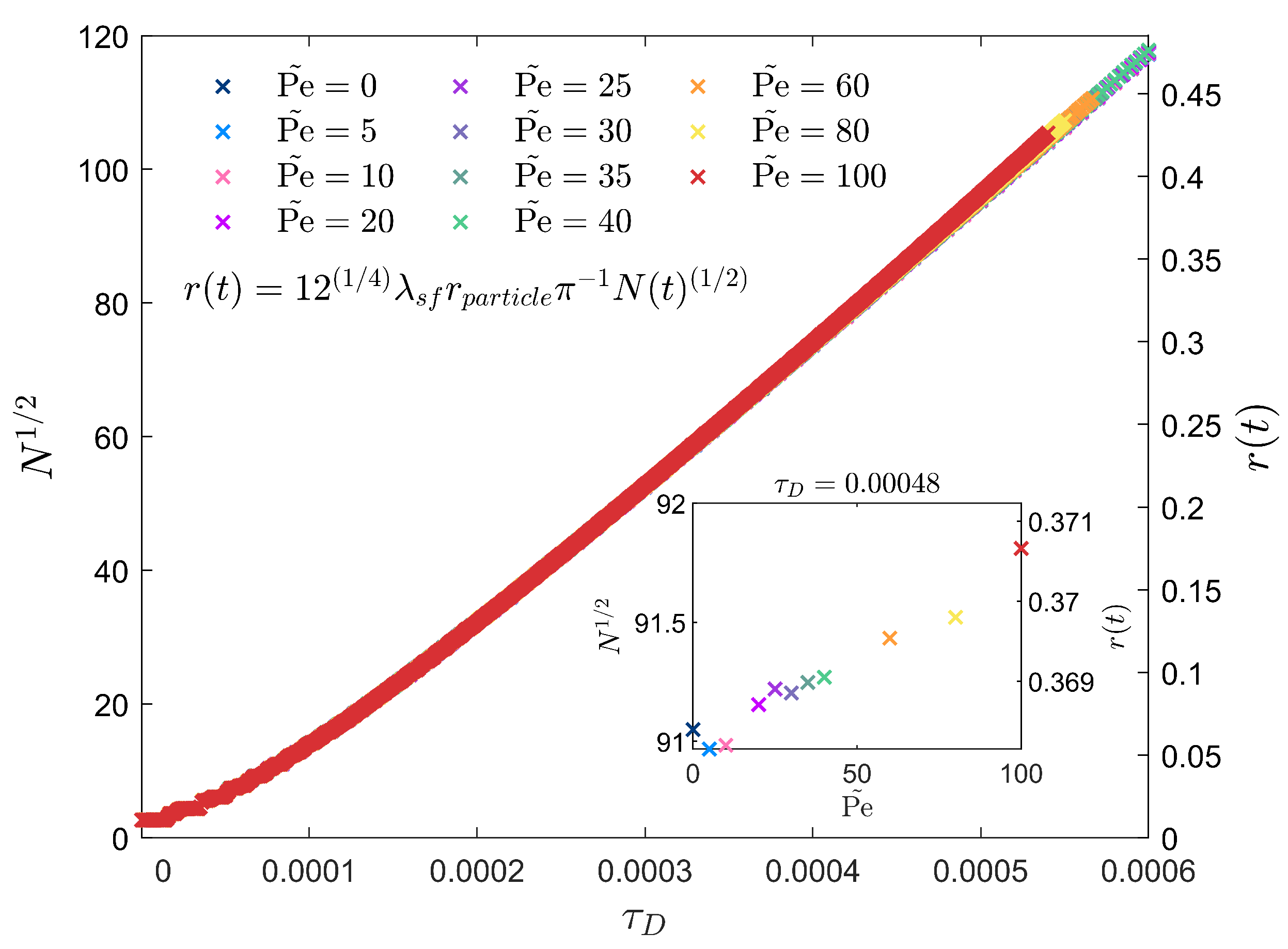
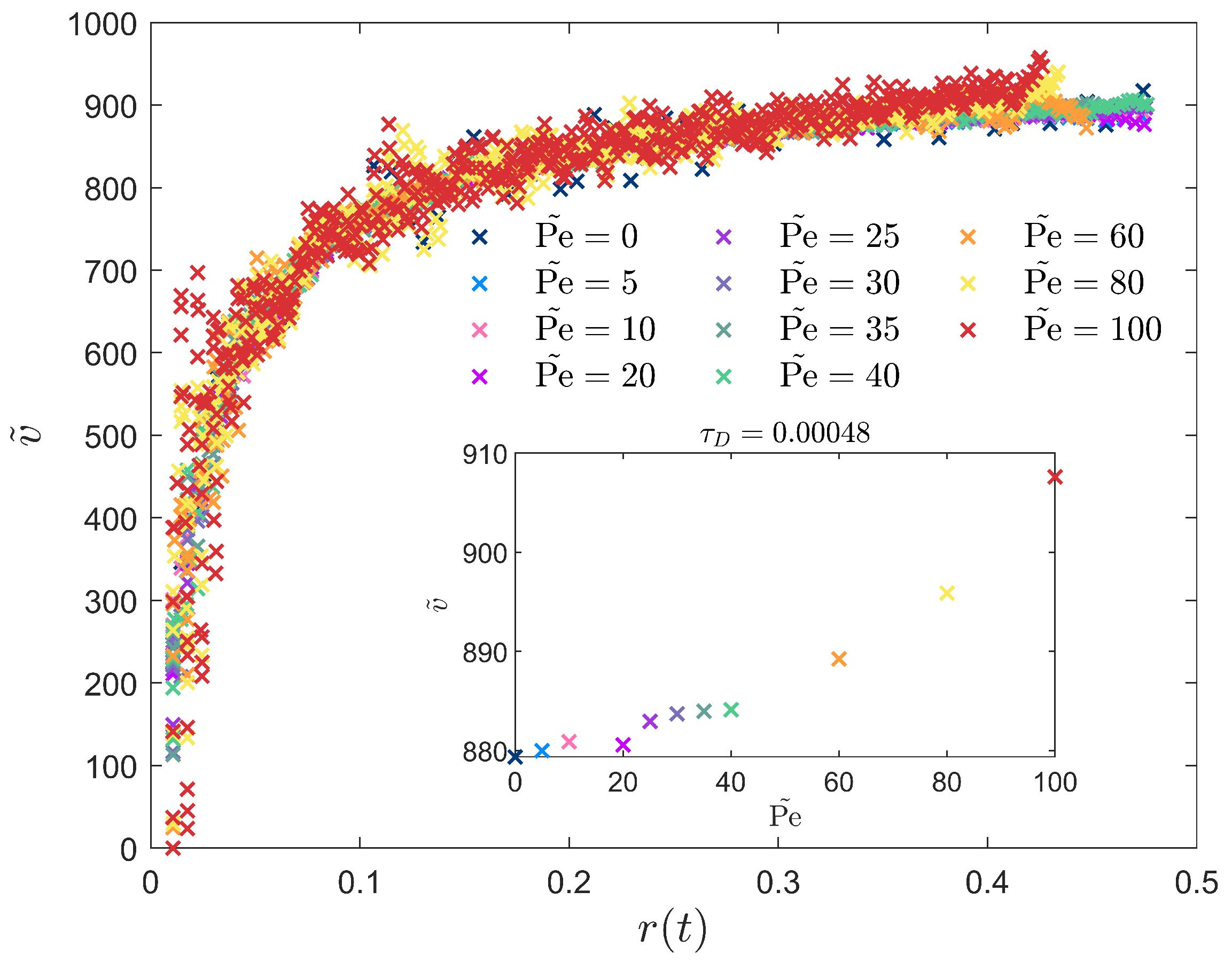
3.2. Peclet-Dependent Crystal Growth

Pe = 100 growth data are shown as an extreme case compared to the Pe = 0 case in Figure 3. To compare the crystal growth in shear flow on the same timescales, the dimensionless convective time scale in Equations (19a)–(20) must be rescaled by Pe . Then, when considering t D = 1 , the time evolution can be compared on the diffusive timescales, τ D . Additionally all effective temperatures are taken at σ = 0.12 , and the initial density at ψ 0 = 0.06 , placing the phase fully in the triangular region according to [34].
The time evolution under simple shear flow when Pe = 100 , Figure 9, shows that the flow causes some anisotropic growth when compared to the no-flow cases in Figure 3 and Figure 4. The anisotropic growth is not as extreme as it would be by going to higher Pe . Because we are studying cases for thin-film flows, it is reasonable to study intermediate Pe . The non-uniform, egg-shaped, anisotropic growth can be explained by the seed being positioned slightly off-center in the flow-field r i n i t i a l L / 2 , rather than exactly r i n i t i a l = L / 2 , meaning the top half experiences the shear much earlier in the development compared to the bottom half. Both hemispheres experience the same shear rates, but interact with the flow-field slightly differently, as the bottom half has more time to develop in the absence of flow; see Figure 2a. The presence of anisotropy suggests that crystal growth is not only shear-rate-dependent, but also flow-field-dependent, meaning that where the crystal interacts with the flow-field should also be considered [50].
As a comparison between flow-mediated and non-advected crystal growth, a linear dimension of the crystal is obtained by taking the square-root of the particle number [16], as plotted in Figure 10. The cluster radii are again extracted using Equation (26). Although the crystal in flow is non-spherical, we see by the fits in Figure 13 that approximating it using spherical equations is a reasonable approximation.
The cluster radii do not change significantly due to moderate shear flow, though after a certain Pe , there is a slight enhancement in the cluster radii (as shown in the inset). The dependence is not uniformly linear as in the non-advected cases; see Figure 5. Additionally, the near-constant behavior at small Pe in Figure 10 indicates a critical Pe , which will be referred to by Pe * . To further analyze how shear impacts crystal growth, the Mermin order-parameters were again studied to visualize structural rearrangement, as shown in Figure 11.
Comparing Figure 11 to the insets of Figure 6, phase change and shear-induced structural rearrangement lead to different behaviors in Ψ 6 and Ψ 4 . The shear-induced rearrangement is more gradual and linear, whereas the effective temperature-induced rearrangement is much more dramatic and non-linear. Figure 11 further supports the presence of Pe * within a range of 20 Pe * < 40 . Additionally, Figure 12 also exhibits near-constant behavior at small Pe , as observed in Figure 10 and Figure 11, corroborating the approximate location of Pe * .
The raw growth velocity behavior in time, Figure 12, obtained from the numerical derivative of r ( t ) , reveals a greater separation with respect to Pe than the radii versus time. The steady state growth velocities, when r ( t ) > 0.32 , were used to fit a line to observe the steady state behavior, and the steady state growth velocities obtained from the fit are plotted at τ ¯ D = 48 in the inset. Upon further inspection, Pe * lies in the range 20 Pe * < 40 . After Pe * , the behavior becomes ’quasi’ linear. However, to explain the root cause of this increased behavior, the growth velocities are decomposed into the crystal plane growth velocities in Section 3.3.

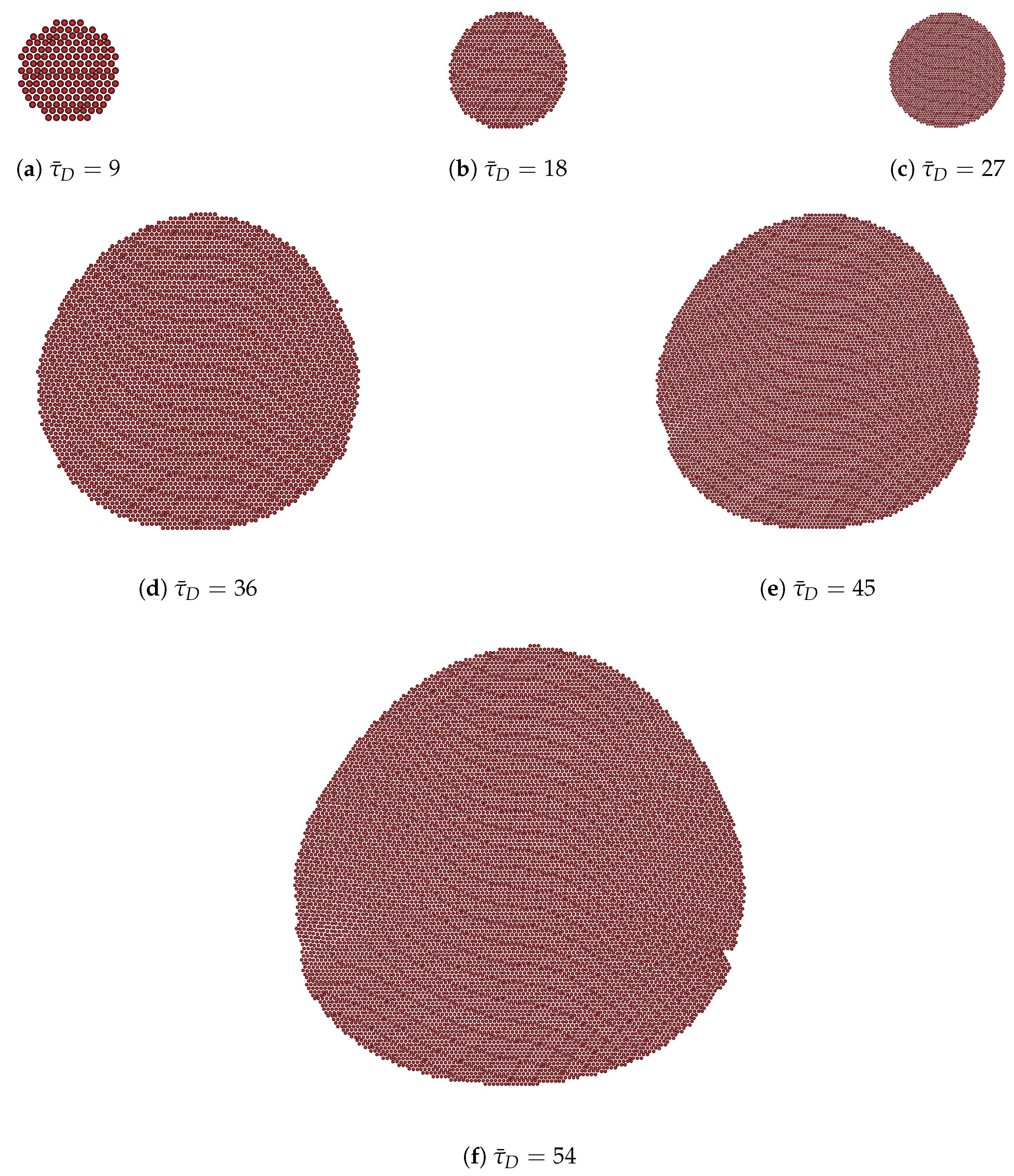
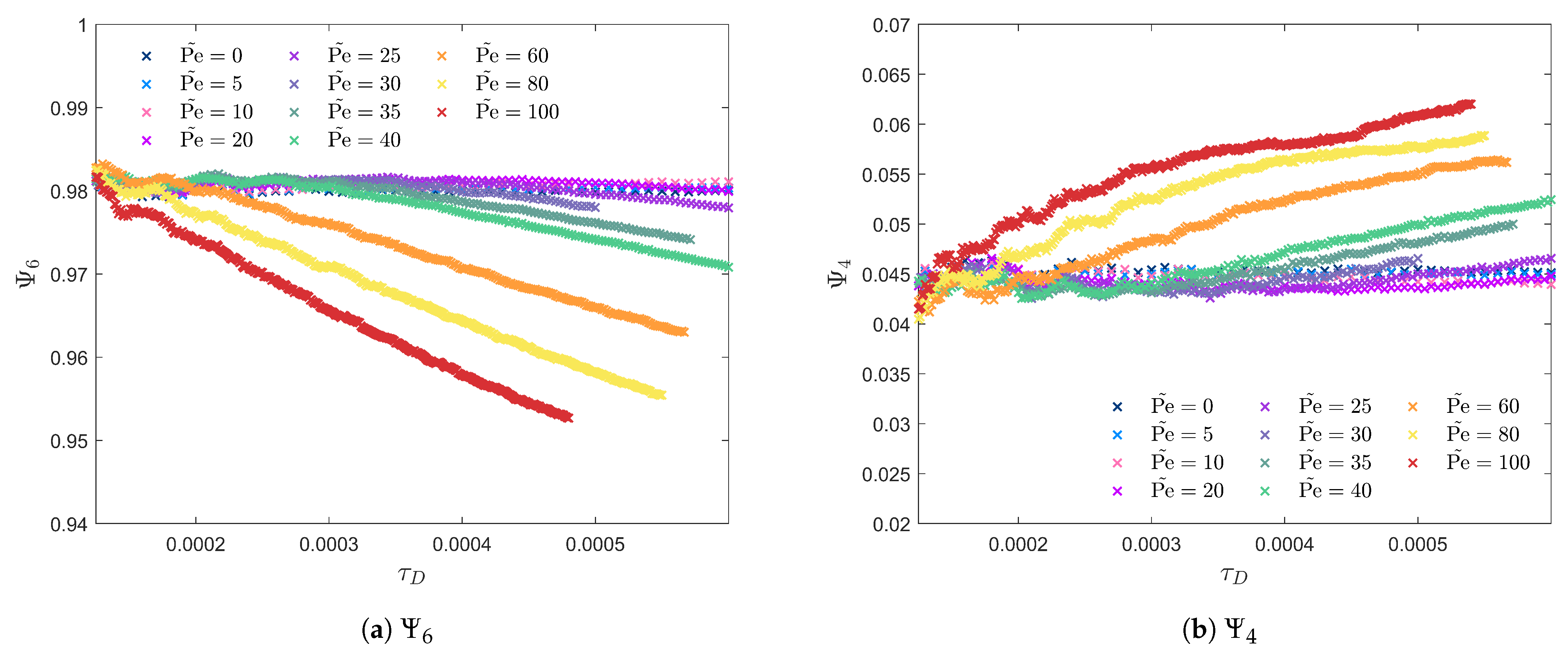
3.3. Crystal Plane Growth Dependence

The 1-D growth information was obtained by taking a cut-line across each crystal plane in the order-parameter (density) field. Obtaining the data for the no-flow case ( σ = 0.12 ) was straightforward, as the crystal growth conformed to long-range ordering in each plane. However, when shear was introduced, the structural rearrangement presented difficulties when obtaining the crystal-plane-dependent growth information, especially at Pe = 100 . Hence, the raw crystal plane growth rate data for the cases with flow could only reliably be obtained for relatively short times, τ ¯ D 25 , or before significant flow-field interactions. The results for Pe = 100 are shown in Figure 13, as a comparison of two extremes.
When first inspecting Figure 13, the no-flow case at Pe = 0 shows no remarkable crystal plane dependence on growth. Alternatively, when Pe = 100 , there is significant crystal plane dependence on growth, with the ( 1 ¯ 1 ¯ ) plane dominating because it is in the direction of the shear (or elongation). Planar-averaged growth velocities are denoted by the black lines, and fit to the 2-D obtained growth velocities shown in the inset. We attribute the slight enhancement seen in Figure 12 to the growth enhancement in the ( 1 ¯ 1 ¯ ) plane.

4. Discussion

It should be noted that PFC simulations are subject to finite size effects when obtaining the data [14,34]. However, the effects are not probed here because we elected to fix the domain size and focus on the effects of shear. Hence, these results should merely be used as a guide when the dimensionless particle diameter is approximately d p a r t i c l e = d p a r t i c l e / L 0.0078 , where L is dimensional box size, or 1/128th of the dimensionless domain size (as 128 was the base scale for the simulation box; see Figure 2a). The dimensionless particle is denoted by r p a r t i c l e = d p a r t i c l e / 2 , to maintain consistency with the notation from Equation (26).
Discretization can have an impact on results. We used d x = 1 8 L b a s e 1 , where L b a s e = 128 , to balance discretization error and computational efficiency; the choice was inspired by [25,34]. Because this is a particle-to-grid method, with oscillatory features, the order-parameter field is very sensitive to grid size. The approximate particle positions are heavily dependent on where the grid crosses the maximum in the order-parameter field; see Figure 2c. As d x 0 , the particle positions could be completely resolved without error, with an increase in computational cost. For future work, adaptive mesh refinement could be utilized to enhance the particle resolution near the cluster to balance computational efficiency and accuracy [18,58]. As confirmation of our discretization, the Mermin order-parameters in the no-flow case at σ = 0.12 , which were calculated using the particle positions obtained in the procedure outlined in Section 2.5, should approach unity as there are no square structures. When referring to Figure 6, it can be seen that the Mermin order-parameter, within reasonable error, approaches unity. Due to the discretization in the flow-field and the order-parameter field, the initial seed was not placed directly in the center of the sheared domain, as shown in Figure 14.
As a consequence, it appears that the off-centering of the crystal seed is the cause of the non-uniform asymmetric growth in Figure 9. It also indicates that at high Pe , the growth is sensitive to location in the flow-field. Hence, the results should be interpreted while also considering finite size effects and the sensitivity to discretization observed in the particle-to-grid simulations. In attempting to uncover the mechanisms of shear-flow on crystal growth, the temperature-dependent crystal growth was first studied. Not only does the dimensionless growth velocity increase with increasing undercooling, as seen in Figure 8, but crystal growth using the PFC equations can be described by Equation (24), as shown by [16]. We further extend the analysis by parameterization according to Equation (25), which could be used to extract the CNT parameters. In doing so, we found that within the same crystal phase, there is an approximately linear increase in N 1 / 2 , r ( t ) , and v with decreasing σ , leading to a proportionality, r ( t ) σ , while in the same phase for 0.1 < σ < 0.12 at ψ 0 = 0.06 (plus some intercept). Furthermore, at σ = 0.09 , the Mermin order-parameter decay showed a steep drop, indicating a phase change that leads to an enhanced growth velocity when the particles prefer the alternative packing. Thermodynamically, this means the free energy in the square phase at σ = 0.09 is much lower than the free energy in the triangular phase at the same σ . Hence, the driving force for crystallization is greater, implying a faster growth rate.
When considering flow, it was found that there is a critical Peclet number that is in the range 20 Pe * < 40 in which the dependence on shear begins to increase approximately linearly, r ( t ) Pe ; see the insets of Figure 10 and Figure 12. Furthermore, above Pe * , the Mermin global order-parameters, Ψ 6 and Ψ 4 , show structural rearrangement due to shear that decays at a much different rate than that for the temperature-induced phase change. In 2009, Wu et al. showed that colloidal hard-sphere suspensions under shear exhibit the same constant decrease in Mermin order-parameter when starting with an initially ordered system, as in Figure 11 [59]. They also reported that compared to quiescent crystallization (the dramatic decay we observe in Figure 6), the gradual decay due to shear points to a different mechanism by which the rearrangement occurs. Additionally, the authors also observed a hexagonal ordering that was always parallel to the flow direction [59], supporting many of the findings reported here. Li et al. confirmed that shear can induce structural transformations and crystal lattice orientation alignment along the shear direction in colloidal crystal experiments with poly(N-iso-propylacrylamide) microgel spheres in aqueous suspensions [60]. Because of the approximate linear dependence and order-parameter decay when comparing to the non-advected cases, it is clear that shear flow is modulating the free energy landscape of the preferred particle packing; see Equations (7a) and (12). Thermodynamically, the temperature, σ , is causing growth enhancement by decreasing the crystallization driving force, Δ G S L , caused by the meta-stable liquid state. At the same temperature, the sheared under-cooled liquid shows slight crystal growth enhancement above Pe * . Therefore, the shear flow must be somehow affecting the crystallization driving force. Rearranging the shear-flow modified CNT equation [8], we find
Δ G ( r ) = 4 3 π r 3 Δ G S L + 2 μ v i s c 2 Pe 2 G 2 t D 2 + 4 π r 2 σ S L ,
where G is the crystal shear modulus and γ ˙ = 2 Pe t D is the shear rate (which was in the original equation reported). Note that Equation (28) is the spherical form of the equation presented in [8]. One can see from Equation (28) that there is a new quasi modulated driving force, Δ G ¯ S L = Δ G S L + 2 μ v i s c 2 Pe 2 G 2 t D 2 . In addition, G ¯ S L , depends on the flow field if Equations (7a) and (12) are combined, ultimately meaning that the flow field and shear rate do indeed affect crystal growth by slightly modifying the driving force. Note that the spatial flow field dependence is elucidated by (12).
There also appeared to be a slight enhancement of crystal growth, as seen when comparing Figure 10 and Figure 12. Upon decomposing the growth velocities into directions of the crystal planes, it was found that the ( 1 ¯ 1 ¯ ) plane, in the direction of the elongational portion of shear flow, shows the fastest growth rate, as seen in Figure 13. Directional-dependent crystal growth velocities, with respect to crystal and flow-field orientation, have been shown to have dependence in a cellular-automota coupled Navier–Stokes model [61,62]. However, their model incorporated no-slip boundary conditions at the crystal surface, did not include wall-driven flows, and also appeared to have a more rigid crystal structure due to it being on a different scale. The crystal growth reported here is early in post-critical nucleus growth and is on the order of magnitude of a cluster of a few particles. Thus, the physics would be slightly different when the fluid phase is interacting with the elasticity and shear modulus of the crystal phase [9]. However, the molecular attachment–detachment mechanism, fundamental to CNT, is a point of comparison as a result of using Equations (24) and (25) (see Appendix C and [53] for more details). In addition, Qazi et al. demonstrated that elongational flow causes plate-like colloidal particles to prefer orienting in the extensional direction, leading to anisotropy in the small-angle neutron scattering patterns [63]. Furthermore, they reported that the particle alignment also has dependence on the flow-field due to flow-misalignment from small differences in pressure or flow-rate in the elongational flow-cell [63]. The extensional flow-induced alignment observed by Qazi et al. not only supports our finding that crystal growth would be enhanced in the elongational flow direction, but also that crystal growth has a similar dependence on the flow field as in Figure 14. Both our and their findings indicate that anisotropy and flow-alignment are not just strain-rate-dependent. More recently, Calabrese et al. decoupled the effects of extensional and shear flows on rigid rodlike particles. They found the particle orientation always aligns with the elongational direction, regardless of the extension rate, where as in shear-flow, the particle orientation is dependent on shear rate [51]. Although the anisotropic particles are more sensitive to alignment, suggested by their Peclet number range 0.01 Pe 10 , their findings also suggest that particle–flow field interaction, flow type, and flow strength are of importance in flow-mediated particle processes [51]. By keeping the equations dimensionless and generalized, we hope that these insights could lead to improved crystal growth optimization during the scale-up of PSC thin-film manufacturing.

5. Conclusions

In summary, we have developed an HXPFC-s2 formalism that describes the over-damped crystallization of Brownian particles described by a hard-sphere-like intermolecular potential, such as the Yukawa potential, as a result of the MSA when connecting the intermolecular potential to the DCF. When neglecting flow, temperature-dependent crystal growth exhibited a linear dependence on Pe , which was enhanced by triangular-to-square phase change. The behavior was further supported by the inner particle averaged Mermin global order-parameter, Ψ 6 and Ψ 4 , behaviors and deviations with the plane-averaged, triangular-phase growth velocity fits to Equation (25) at σ = 0.09 . When including flow, crystal growth exhibited near constant behavior at small Pe , differing with the monotonically increasing growth with decreasing temperature, σ . However, above Pe * , shear-flow caused a slight enhancement in the cluster radii, with the approximately linear scaling being similar to the linear scaling observed when decreasing the effective temperature, with r ( t ) Pe . The crystal structural rearrangement, indicated by Ψ 6 and Ψ 4 , in the intermediate Pe range was not as extreme as a temperature-induced, σ , phase change, but is present and increases with increasing Pe . Furthermore, the slight shear-flow enhancement can be attributed to the crystal plane in the closest direction of the elongational portion of shear-flow. By considering the flow-modulated crystal growth presented in this work, we expect our findings to guide another optimization dimension for scalable PSC thin-film manufacturing techniques. For future work, the full two-way coupling will be implemented by including particle–fluid viscosity differences to capture the no-slip boundary conditions around the growing cluster [18,45]. In doing so, the effects of Eu and Re coupling on crystal growth can be fully analyzed, thereby offering a wider range of dimensionless parameters for application to PSC thin-film technologies.

Author Contributions

Conceptualization, L.C.W., R.R.R. and Z.L.L.; methodology, L.C.W. and Z.L.L.; software, L.C.W.; validation, L.C.W. and Z.L.L.; formal analysis, L.C.W. and Z.L.L.; investigation, L.C.W., R.R.R. and Z.L.L.; resources, R.R.R. and Z.L.L.; data curation, L.C.W.; writing—original draft preparation, L.C.W.; writing—review and editing, L.C.W., T.D.J., R.R.R. and Z.L.L.; visualization, L.C.W.; supervision, Z.L.L.; project administration, R.R.R. and Z.L.L.; funding acquisition, R.R.R. and Z.L.L. All authors have read and agreed to the published version of the manuscript.

Funding

This research was funded by Sandia National Laboratories and FAMU-FSU Start-up Fund.

Institutional Review Board Statement

Not applicable.

Informed Consent Statement

Not applicable.

Data Availability Statement

Data are contained within the article.

Acknowledgments

This work was supported by the Laboratory Directed Research and Development program at Sandia National Laboratories, a multi-mission laboratory managed and operated by National Technology and Engineering Solutions of Sandia, LLC, a wholly owned subsidiary of Honeywell International Inc. for the U.S. Department of Energy’s National Nuclear Security Administration under contract DE-NA0003525. This written work is authored by an employee of NTESS. The employee, not NTESS, owns the right, title and interest in and to the written work and is responsible for its contents. Any subjective views or opinions that might be expressed in the written work do not necessarily represent the views of the U.S. Government. The publisher acknowledges that the U.S. Government retains a non-exclusive, paid-up, irrevocable, world-wide license to publish or reproduce the published form of this written work or allow others to do so, for U.S. Government purposes. The DOE will provide public access to results of federally sponsored research in accordance with the DOE Public Access Plan. This work used Stampede 3 at Texas Advanced Computing Center (TACC) The University of Texas at Austin through the CHM240001 allocation from the Advanced Cyberinfrastructure Coordination Ecosystem: Services & Support (ACCESS) program, which is supported by U.S. National Science Foundation grants No. 2138259, 2138286, 2138307, 2137603, and 2138296. The computing for this project was also partially performed on the high-performance computing (HPC) cluster at the Florida State University Research Computing Center supported by the FAMU-FSU Start-up Fund. The authors would also like to thank Ken Elder, Nikolas Provatas, and Petri Hirvonen for their suggestions on Phase Field Crystal implementation, as well as Christine Roberts and Tyler Kennelly for their valuable input and feedback.

Conflicts of Interest

The authors declare no conflicts of interest.

Abbreviations

The following abbreviations are used in this manuscript:
HXPFC-s2Hydrodynamic Structural Phase Field Crystal semi-two-way Coupled
PFCPhase Field Crystal
XPFCStructural Phase Field Crystal
DCFDirect Correlation Function
DDFTDynamic Density Functional Theory
HNCHypernetted Chain
MSAMean Spherical Approximation
RPARandom Phase Approximation

Appendix A. General HXPFC Formalism Derivation

Appendix A.1. Free Energy Functional

For more information on the following derivation of the free energy functional from classical statistical mechanics, see [11,36]. Additionally, if a variable is bolded, r , it is a vector quantity containing information in all directions, whereas if it is italicized only, r, it is either a variable for a single direction or a scalar quantity. We begin with the canonical partition function in phase space, which contains all relevant thermodynamic information.
Z = 1 h 3 N N ! d p N d r N e β p 2 2 m + β U n b ( r N ) .
After integrating Equation (A1) over the momenta of the system,
Z = 1 λ t h 3 N N ! d r N e β U n b ( r N )
where λ t h = h 2 π m k B T is the thermal de Broglie wavelength.
Using Equation (A3), the Helmholtz free energy can be obtained via:
F = k B T ln 1 λ t h 3 N N ! d r N e β U n b ( r N )
Considering ρ ( r ) = i N δ ( r r i ) , N = d r ρ ( r ) , and that in the thermodynamic limit Stirling’s approximation N ! = N ln ( N ) N [36] applies, and multiplying by ( V / V ) N inside of the parentheses, Equation (A3) becomes
F [ ρ ( r ) ] = k B T d r ρ ( r ) ln ( λ t h 3 ρ ( r ) ) 1 + F E X [ ρ ( r ) ]
The excess free energy functional is left general in Equation (A4). Then, the functional Taylor expansion is performed about a reference density [11,17,23,36] ρ ( r ) = ρ r e f + Δ ρ ( r )
F E X [ ρ ( r ) ] F E X [ ρ r e f ] + d r δ F E X δ ρ ( r ) Δ ρ ( r ) + 1 2 d r d r Δ ρ ( r ) δ 2 F E X δ ρ ( r ) δ ρ ( r ) Δ ρ ( r ) +
Understanding that C ( n ) ( r 1 , , r n ) = β δ ( n ) F δ ρ ( r 1 ) δ ρ ( r n ) represents the n-particle direct correlation function, keeping the total number of particles constant, d r Δ ρ ( r ) = 0 , and neglecting F E X [ ρ r e f ]
F [ ρ ( r ) ] = k B T d r ρ ( r ) ln ( λ t h 3 ρ ( r ) ) 1 k B T 2 d r d r Δ ρ ( r ) C ( 2 ) ( | r r | ) Δ ρ ( r )
Converting into PFC coordinates, we must take ρ ( r ) = ρ r e f ( 1 + ψ ( r ) ) . Therefore, ψ ( r ) = ( ρ ( r ) / ρ r e f 1 ) . After changing variables,
F [ ψ ( r ) ] = ρ r e f k B T d r ( 1 + ψ ( r ) ) ln [ λ t h 3 ( 1 + ψ ( r ) ) ] 1   k B T 2 ρ r e f d r d r ψ ( r ) C ( 2 ) ( | r r | ) ψ ( r )
After Taylor expanding the ln [ λ t h 3 ( 1 + ψ ( r ) ) ] and truncating the fifth- and higher-order terms [24], neglecting the Thermal de broglie wavelength, and collecting like terms,
F [ ψ ( r ) ] ρ r e f k B T = d r ψ 2 ( r ) 2 ψ 3 ( r ) 6 + ψ 4 ( r ) 12 1 2 d r ψ ( r ) C ( 2 ) ( | r r | ) ψ ( r )   + d r ψ ( r ) U ( r ) e x t k B T .
giving the free energy functional in the XPFC formalism, including a general external potential. We note that traditionally, the free energy functional is derived from the grand canonical ensemble. However, as discussed at length by Marconi and Tarazona, approximating a canonical ensemble with a free energy functional can lead to errors [22].

Appendix A.2. Advected PFC Equation

In the full derivation of the advection PFC equation, we begin with the over-damped Lagevin equation of motion for Brownian particles that is in the presence of a flow field [17,18,21,22,23]:
d r i d t = u ( r i , t ) 1 k B T i = 1 N U n b ( | r i r j | ) + 2 ω m i k B T ξ i ( t ) ,
ξ i ( t ) = 0
ξ i m ( t ) ξ j n ( t ) = 2 ω m i k B T δ i j δ m n δ ( t t )
where ω is the damping frequency, m i is the atomic mass of particle i, u i is the fluid velocity at particle i, and U n b ( | r i r j | ) is the non-bonded pair-wise intermolecular potential.
The individual and overall number densities [21] are
ρ i ( r i , t ) = δ ( r i ( t ) r )
ρ ( r , t ) = i = 1 N ρ i ( r , t )
Following [21,35], an arbitrary test function f [ r i ( t ) ] as a function of particle position, r i ( t ) , is used to make the particle-to-grid transformation, which has the following properties:
f [ r i ( t ) ] = d r ρ i ( r , t ) f ( r )
f [ r i ( t ) ] t = d r ρ i t f ( r )
The test function can be Taylor expanded and rearranged to the form of a stochastic integral Equation [35]. After using Ito’s Lemma [21,22], and matching terms, one obtains
f [ r i ( t ) ] t = d r ρ i ( r , t ) [ f ( r ) · u ( r i , t )   1 ω m i f ( r ) · j = 1 N U n b ( | r i r j | ) + k B T ω m i 2 f ( r ) + 2 k B T ω m i f ( r ) · ξ ( t ) ]
After integration by parts and neglecting the surface integrals that arise [35] and rearranging to the form
d r f ( r ) [ ρ i ( r , t ) t + ( ρ i ( r , t ) u ( r i , t ) )   1 ω m i · ( ρ i ( r , t ) j N U n b ( | r i r j | ) ) k B T ω m i 2 ρ i ( r , t )   + 2 k B T ω m i · ( ρ ( r , t ) ξ ( t ) ) ] = 0
Because we set f ( r ) to be an arbitrary function [21,22,35], allowing the term in brackets to equal zero, and summing over all particles, we obtain
ρ ( r , t ) t + ( ρ ( r , t ) u ( r , t ) )   = 1 ω m · ( ρ ( r , t ) d r U n b ( | r r | ) ρ ( r , t ) ) + k B T ω m 2 ρ i ( r , t )   + 2 k B T ω m ρ ( r , t ) · ξ ( t )
where after summation the number particle density, ρ ( r , t ) , allows the atomic mass of particle i, m i , to be interchangeable with atomic mass, m, from Table 1.
After utilizing (11)–(13) and replacing terms in Equation (A14) [17,21,22,23], we obtain
ρ ( r , t ) t + · ( ρ ( r , t ) u ( r , t ) ) = · M ( r ) δ F ¯ [ ρ ( r ) ] δ ρ + · 2 M ( r ) ξ ( t )
where M ( r ) = k B T ω m ρ ( r , t ) and F ¯ = F / k B T . Equation (A15) is similar in form to the advected DDFT reported in [31]. However, when converting to PFC variables, the mobility, M, is treated as a constant. Using the order-parameter defined with ρ ( r ) = ρ r e f ( 1 + ψ ( r ) ) , Equation (A15) can be placed in PFC form
ψ ( r , t ) t + · ( ψ ( r , t ) u ( r , t ) ) = M 2 δ F [ ψ ( r ) ] δ ψ + · 2 M ξ ( t ) .
In addition, expanding the advection term in Equation (A16) and using the incompressible continuity equation, Equation (5b), yields Equation (6).

Appendix A.3. Navier–Stokes Coupling

To derive the momentum coupling in Equation (5a), we begin with Equation (A12) and observe that Ito’s equation is effectively a chain rule:
f [ r i ( t ) ] t = f [ r i ( t ) ] · r i t = d r ρ i ( r , t ) [ f ( r ) · u ( r i , t )   1 ω m i f ( r ) · j = 1 N U n b ( | r i r j | ) + k B T ω m i 2 f ( r )   + 2 k B T ω m i f ( r ) · ξ ( t ) ]
Now, the advection term can be subtracted from the right-hand side of Equation (A17), and utilizing Equations (A11a) and (A11b), the equation becomes
d r ρ i ( r , t ) f ( r ) · v i ( r , t ) u ( r i , t ) =   d r ρ i ( r , t ) [ 1 ω m i f ( r ) · j = 1 N U n b ( | r i r j | ) + k B T ω m i 2 f ( r )   + 2 k B T ω m i f ( r ) · ξ ( t ) ]
where r i t = v i is the velocity of particle i.
Integrating by parts, again neglecting the surface terms, and summing over all particles gives
d r f ( r ) · ρ ( r , t ) ( v ( r , t ) u ( r , t ) ) = d r f ( r ) [ 1 ω m · ( ρ ( r , t ) d r U n b ( | r r | ) ρ ( r , t ) ) + k B T ω m 2 ρ ( r , t ) + 2 k B T ω m · ( ρ ( r , t ) ξ ( t ) ) ]
By using the same argument that led to Equation (A14),
· ρ ( r , t ) ( v ( r , t ) u ( r , t ) ) =   · [ 1 ω m ( ρ ( r , t ) d r U n b ( | r r | ) ρ ( r , t ) ) + k B T ω m ρ ( r , t )   + 2 k B T ω m ( ρ ( r , t ) ξ ( t ) ) ]
By considering only the terms in brackets, and algebraic rearrangement, we see
ω m ρ ( r , t ) ( v ( r , t ) u ( r , t ) ) =   ( ρ ( r , t ) d r U n b ( | r r | ) ρ ( r , t ) ) + k B T ρ ( r , t )   + 2 k B T ω m ( ρ ( r , t ) ξ ( t ) )
We note that the left-hand side of Equation (A21) is the same as Equation (17). By using Ito’s Lemma as a particle-to-grid transformation, and utilizing Equations (11)–(13), Equation (A21) becomes
ω m ρ ( r , t ) ( v ( r , t ) u ( r , t ) ) = ρ ( r , t ) δ F δ ρ + 2 k B T ω m ( ρ ( r , t ) ξ ( t ) )
yielding the full forcing term, with thermal noise, presented in Equation (18) and reported in [18,29].

Appendix B. Dimensionless HXPFC-s2 Form Derivation

For Appendix B.1 and Appendix B.2, we begin with Equations (5a)–(6). In both sections, dimensionless values are denoted by x .

Appendix B.1. Convective Timescale

The dimensionless quantities used to normalize are:
u = u / u 0
= L
P = P ¯ / P 0
t c = L / u 0
τ = t / t c
ν = Δ ν / ν 0 + 1
F [ ψ ( r ) ] = F [ ψ ( r ) ] ρ r e f k B T

Appendix B.2. Diffusive Timescale

The dimensionless quantities used to normalize are the same as in Appendix B.1, except the PFC time scale is now normalized by the diffusive timescale. We also report the final form of the dimensionless equations normalized by the diffusive timescales for completeness.
The dimensionless time quantities used to normalize on the diffusive time scale are:
t D = L 2 / M
τ D = t / t D
u τ D + Pe · ( u u ) = Eu Pe P + Sc · ν u + ( u ) T + De ψ δ F [ ρ ( r ) ] δ ψ
· u = 0
ψ τ D + Pe u · ψ = 2 δ F [ ρ ( r ) ] δ ρ + 2 t D · ξ ( t )

Appendix C. Derivation of Theoretical Growth Rate Equation

This is a restatement of Kelton and Greer’s 1985 equation [53,54,55], describing the growth of a spherical cluster during crystallization.
Using the reaction equation describing a cluster of particles gaining one particle, with the chance of the larger cluster to lose one particle [54],
E n + E 1 k n + 1 k n + E n + 1
The reaction rate constants are as follows [54,55]:
k n + = 6 D λ 2 O n exp Δ G 2 k B T
k n = 6 D λ 2 O n 1 exp Δ G 2 k B T
where D is the diffusivity of the interface and O n = 4 n 2 / 3 is the number of sites on the cluster [53,55]. Additionally, because the cluster is considered post-critical, it can be shown using [54] the equation,
Δ G = n Δ G S L + ( 36 π ) 1 / 3 ( v ¯ n ) 2 / 3 σ S L
and Equation (21), that at the critical radius,
n * = 4 π 3 V ¯ r * 3 .
By using the reaction describing the cluster gaining one particle, from Equation (A27), the kinetic equation becomes [53]
d n d t = 6 D λ 2 4 n 2 / 3 exp Δ G 2 k B T exp Δ G 2 k B T
After rearrangement, Equation (A32) becomes
d n d t = 6 D λ 2 8 n 2 / 3 sinh Δ G 2 k B T
Using both Equations (A29) and (A30), and after rearrangement, Equation (A32) becomes
d r d t = 16 D λ 2 3 V ¯ 4 π 1 / 3 sinh V ¯ 2 k B T Δ G S L + 3 σ S L r .
Equation (A33) is slightly modified from the original form reported by Kelton and Greer in [53]. We note that using Equation (A30) and rearranging Equation (21), the 3 comes from factoring out 4 3 π r 3 , rather than the 2 reported by [53]. However, because we are fitting the equations to data, this is a minor concern when using the originally reported equation, Equation (24) and in PFC units, Equation (25). Additionally, the n term that comes out of the parentheses inside the brackets of Equation (A33) is set to unity because we are describing the energy to gain one particle. Finally, the negative sign has been added to account for the argument inside the brackets being negative [53], since the equation best describes a seed that is size r 1.5 r * ; see Figure 1 [54,55]. Utilizing V ¯ = 1 ρ r e f and v = d r d t λ 2 D V ¯ ( 1 / 3 ) , Equation (A34) can be placed in PFC units:
v = 16 3 4 π 1 / 3 sinh 1 2 Δ G S L + 3 2 σ S L r .

References

  1. Yang, H.; Wang, H.; Wang, K.; Liu, D.; Zhao, L.; Chen, D.; Zhu, W.; Zhang, J.; Zhang, C. Recent Progress of Film Fabrication Process for Carbon-Based All-Inorganic Perovskite Solar Cells. Crystals 2023, 13, 679. [Google Scholar] [CrossRef]
  2. Soto-Montero, T.; Soltanpoor, W.; Morales-Masis, M. Pressing challenges of halide perovskite thin film growth. APL Mater. 2020, 8, 110903. [Google Scholar] [CrossRef]
  3. Li, Z.; Klein, T.R.; Kim, D.H.; Yang, M.; Berry, J.J.; Van Hest, M.F.A.M.; Zhu, K. Scalable fabrication of perovskite solar cells. Nat. Rev. Mater. 2018, 3, 18017. [Google Scholar] [CrossRef]
  4. Weerasinghe, H.C.; Macadam, N.; Kim, J.E.; Sutherland, L.J.; Angmo, D.; Ng, L.W.T.; Scully, A.D.; Glenn, F.; Chantler, R.; Chang, N.L.; et al. The first demonstration of entirely roll-to-roll fabricated perovskite solar cell modules under ambient room conditions. Nat. Commun. 2024, 15, 1656. [Google Scholar] [CrossRef]
  5. Guo, Q.; Gong, X.; Shen, Z.; Hao, X.; Zhang, J. Numerical Simulation on Preparing Uniform and Stable Perovskite Wet Film in Slot-Die Coating Process. ACS Omega 2023, 8, 19547–19555. [Google Scholar] [CrossRef]
  6. Wang, X.; Zhou, Y. Research on Single Crystal Preparation via Dynamic Liquid Phase Method. Crystals 2023, 13, 1150. [Google Scholar] [CrossRef]
  7. Małysiak, A.; Orda, S.; Drzazga, M. Influence of Supersaturation, Temperature and Rotational Speed on Induction Time of Calcium Sulfate Crystallization. Crystals 2021, 11, 1236. [Google Scholar] [CrossRef]
  8. Mura, F.; Zaccone, A. Effects of shear flow on phase nucleation and crystallization. Phys. Rev. E 2016, 93, 042803. [Google Scholar] [CrossRef]
  9. Elder, K.R.; Katakowski, M.; Haataja, M.; Grant, M. Modeling Elasticity in Crystal Growth. Phys. Rev. Lett. 2002, 88, 245701. [Google Scholar] [CrossRef] [PubMed]
  10. Elder, K.R.; Grant, M. Modeling elastic and plastic deformations in nonequilibrium processing using phase field crystals. Phys. Rev. E 2004, 70, 051605. [Google Scholar] [CrossRef]
  11. Ramakrishnan, T.V.; Yussouff, M. First-principles order-parameter theory of freezing. Phys. Rev. B 1979, 19, 2775–2794. [Google Scholar] [CrossRef]
  12. Elder, K.R.; Provatas, N.; Berry, J.; Stefanovic, P.; Grant, M. Phase-field crystal modeling and classical density functional theory of freezing. Phys. Rev. B 2007, 75, 064107. [Google Scholar] [CrossRef]
  13. Gao, N.; Zhao, Y.; Xia, W.; Liu, Z.; Lu, X. Phase-Field Crystal Studies on Grain Boundary Migration, Dislocation Behaviors, and Topological Transition under Tension of Square Polycrystals. Crystals 2023, 13, 777. [Google Scholar] [CrossRef]
  14. Hirvonen, P.; Ervasti, M.M.; Fan, Z.; Jalalvand, M.; Seymour, M.; Vaez Allaei, S.M.; Provatas, N.; Harju, A.; Elder, K.R.; Ala-Nissila, T. Multiscale modeling of polycrystalline graphene: A comparison of structure and defect energies of realistic samples from phase field crystal models. Phys. Rev. B 2016, 94, 035414. [Google Scholar] [CrossRef]
  15. Ankudinov, V.; Galenko, P.K. Noise-Induced Defects in Honeycomb Lattice Structure: A Phase-Field Crystal Study. Crystals 2023, 14, 38. [Google Scholar] [CrossRef]
  16. Podmaniczky, F.; Gránásy, L. Nucleation and Post-Nucleation Growth in Diffusion-Controlled and Hydrodynamic Theory of Solidification. Crystals 2021, 11, 437. [Google Scholar] [CrossRef]
  17. Praetorius, S.; Voigt, A. A Phase Field Crystal Approach for Particles in a Flowing Solvent. Macromol. Theory Simul. 2011, 20, 541–547. [Google Scholar] [CrossRef]
  18. Praetorius, S.; Voigt, A. A Navier-Stokes phase-field crystal model for colloidal suspensions. J. Chem. Phys. 2015, 142, 154904. [Google Scholar] [CrossRef]
  19. Heinonen, V.; Achim, C.; Kosterlitz, J.; Ying, S.C.; Lowengrub, J.; Ala-Nissila, T. Consistent Hydrodynamics for Phase Field Crystals. Phys. Rev. Lett. 2016, 116, 024303. [Google Scholar] [CrossRef]
  20. Podmaniczky, F.; Gránásy, L. Molecular scale hydrodynamic theory of crystal nucleation and polycrystalline growth. J. Cryst. Growth 2022, 597, 126854. [Google Scholar] [CrossRef]
  21. Dean, D.S. Langevin equation for the density of a system of interacting Langevin processes. J. Phys. A Math. Gen. 1996, 29, L613–L617. [Google Scholar] [CrossRef]
  22. Marconi, U.M.B.; Tarazona, P. Dynamic density functional theory of fluids. J. Chem. Phys. 1999, 110, 8032–8044. [Google Scholar] [CrossRef]
  23. Van Teeffelen, S.; Backofen, R.; Voigt, A.; Löwen, H. Derivation of the phase-field-crystal model for colloidal solidification. Phys. Rev. E 2009, 79, 051404. [Google Scholar] [CrossRef]
  24. Emmerich, H.; Löwen, H.; Wittkowski, R.; Gruhn, T.; Tóth, G.I.; Tegze, G.; Gránásy, L. Phase-field-crystal models for condensed matter dynamics on atomic length and diffusive time scales: An overview. Adv. Phys. 2012, 61, 665–743. [Google Scholar] [CrossRef]
  25. Greenwood, M.; Provatas, N.; Rottler, J. Free Energy Functionals for Efficient Phase Field Crystal Modeling of Structural Phase Transformations. Phys. Rev. Lett. 2010, 105, 045702. [Google Scholar] [CrossRef]
  26. Greenwood, M.; Rottler, J.; Provatas, N. Phase-field-crystal methodology for modeling of structural transformations. Phys. Rev. E 2011, 83, 031601. [Google Scholar] [CrossRef] [PubMed]
  27. Cavaterra, C.; Grasselli, M.; Mehmood, M.A.; Voso, R. Analysis of a Navier–Stokes phase-field crystal system. Nonlinear Anal. Real World Appl. 2025, 83, 104263. [Google Scholar] [CrossRef]
  28. An, J.; Zhang, J.; Yang, X. A novel second-order time accurate fully discrete finite element scheme with decoupling structure for the hydrodynamically-coupled phase field crystal model. Comput. Math. Appl. 2022, 113, 70–85. [Google Scholar] [CrossRef]
  29. Yang, X.; He, X. Numerical approximations of flow coupled binary phase field crystal system: Fully discrete finite element scheme with second-order temporal accuracy and decoupling structure. J. Comput. Phys. 2022, 467, 111448. [Google Scholar] [CrossRef]
  30. Yang, J.; Kim, J. Consistent energy-stable method for the hydrodynamics coupled PFC model. Int. J. Mech. Sci. 2023, 241, 107952. [Google Scholar] [CrossRef]
  31. Rauscher, M. DDFT for Brownian particles and hydrodynamics. J. Phys. Condens. Matter 2010, 22, 364109. [Google Scholar] [CrossRef] [PubMed]
  32. Archer, A.J. Dynamical density functional theory for molecular and colloidal fluids: A microscopic approach to fluid mechanics. J. Chem. Phys. 2009, 130, 014509. [Google Scholar] [CrossRef] [PubMed]
  33. Willis, L.W.; Rao, R.R.; Liu, L.L. Towards a multiscale computational framework for simulating flow-mediated crystallization based on phase-field crystal formalisms. In Proceedings of the 16th World Congress on Computational Mechanics and 4th Pan American Congress on Computational Mechanics, Vancouver, BC, Canada, 21–26 July 2024. [Google Scholar] [CrossRef]
  34. Huang, Y.; Wang, J.; Wang, Z.; Li, J.; Guo, C.; Guo, Y.; Yang, Y. Existence and forming mechanism of metastable phase in crystallization. Comput. Mater. Sci. 2016, 122, 167–176. [Google Scholar] [CrossRef]
  35. Gardiner, C.W. Handbook of Stochastic Methods: For Physics, Chemistry and the Natural Sciences, study ed., 2. ed., 6. print ed.; Number 13 in Springer Series in Synergetics; Springer: Berlin/Heidelberg, Germany, 2002. [Google Scholar]
  36. Hansen, J.P.; McDonald, I.R. Theory of Simple Liquids: With Applications to Soft Matter, 4th ed.; Elsevier/AP: Amstersdam, The Netherlands, 2013. [Google Scholar]
  37. Liu, Z.; Zhu, Y.; Clausen, J.R.; Lechman, J.B.; Rao, R.R.; Aidun, C.K. Multiscale method based on coupled lattice-Boltzmann and Langevin-dynamics for direct simulation of nanoscale particle/polymer suspensions in complex flows. Int. J. Numer. Methods Fluids 2019, 91, 228–246. [Google Scholar] [CrossRef]
  38. Rasaiah, J.C.; Card, D.N.; Valleau, J.P. Calculations on the “Restricted Primitive Model” for 1–1 Electrolyte Solutions. J. Chem. Phys. 1972, 56, 248–255. [Google Scholar] [CrossRef]
  39. Solana, J.R. Perturbation Theories for the Thermodynamic Properties of Fluids and Solids; CRC Press, Taylor & Francis Group: Boca Raton, FL, USA, 2013. [Google Scholar]
  40. Te Vrugt, M.; Löwen, H.; Wittkowski, R. Classical dynamical density functional theory: From fundamentals to applications. Adv. Phys. 2020, 69, 121–247. [Google Scholar] [CrossRef]
  41. Lovett, R.; Mou, C.Y.; Buff, F.P. The structure of the liquid–vapor interface. J. Chem. Phys. 1976, 65, 570–572. [Google Scholar] [CrossRef]
  42. Henderson, D.; Boda, D. Mean spherical approximation for the Yukawa fluid radial distribution function. Mol. Phys. 2011, 109, 1009–1013. [Google Scholar] [CrossRef]
  43. Kundu, M.; Howard, M.P. Dynamic density functional theory for drying colloidal suspensions: Comparison of hard-sphere free-energy functionals. J. Chem. Phys. 2022, 157, 184904. [Google Scholar] [CrossRef] [PubMed]
  44. Taira, K.; Colonius, T. The immersed boundary method: A projection approach. J. Comput. Phys. 2007, 225, 2118–2137. [Google Scholar] [CrossRef]
  45. Tanaka, H.; Araki, T. Simulation Method of Colloidal Suspensions with Hydrodynamic Interactions: Fluid Particle Dynamics. Phys. Rev. Lett. 2000, 85, 1338–1341. [Google Scholar] [CrossRef] [PubMed]
  46. Sanz, E.; Vega, C.; Espinosa, J.R.; Caballero-Bernal, R.; Abascal, J.L.F.; Valeriani, C. Homogeneous Ice Nucleation at Moderate Supercooling from Molecular Simulation. J. Am. Chem. Soc. 2013, 135, 15008–15017. [Google Scholar] [CrossRef]
  47. Fletcher, C.A.J. Computational Techniques for Fluid Dynamics 2: Specific Techniques for Different Flow Categories; Scientific Computation, Springer: Berlin/Heidelberg, Germany, 1991. [Google Scholar] [CrossRef]
  48. Trefethen, L.N. Spectral Methods in MATLAB; Software, Environments, Tools; Society for Industrial and Applied Mathematics: Philadelphia, PA, USA, 2000. [Google Scholar]
  49. Strikwerda, J.C. Finite Difference Schemes and Partial Differential Equations, 2nd ed.; Society for Industrial and Applied Mathematics: Philadelphia, PA, USA, 2004. [Google Scholar]
  50. Qu, G.; Zhao, X.; Newbloom, G.M.; Zhang, F.; Mohammadi, E.; Strzalka, J.W.; Pozzo, L.D.; Mei, J.; Diao, Y. Understanding Interfacial Alignment in Solution Coated Conjugated Polymer Thin Films. ACS Appl. Mater. Interfaces 2017, 9, 27863–27874. [Google Scholar] [CrossRef] [PubMed]
  51. Calabrese, V.; Haward, S.J.; Shen, A.Q. Effects of Shearing and Extensional Flows on the Alignment of Colloidal Rods. Macromolecules 2021, 54, 4176–4185. [Google Scholar] [CrossRef]
  52. Kristupas, T. peaks2-find peaks in 2D data without additional toolbox.
  53. Kelton, K.; Greer, A. Interpretation of Experimental Measurements of Transient Nucleation. In Rapidly Quenched Metals; Elsevier: Amsterdam, The Netherlands, 1985; pp. 223–226. [Google Scholar] [CrossRef]
  54. Kelton, K. Crystal Nucleation in Liquids and Glasses. In Solid State Physics; Elsevier: Amsterdam, The Netherlands, 1991; Volume 45, pp. 75–177. [Google Scholar] [CrossRef]
  55. Kelton, K.; Greer, A. Transient nucleation effects in glass formation. J. Non-Cryst. Solids 1986, 79, 295–309. [Google Scholar] [CrossRef]
  56. Mermin, N.D. Crystalline Order in Two Dimensions. Phys. Rev. 1968, 176, 250–254. [Google Scholar] [CrossRef]
  57. Radhakrishnan, R.; Trout, B.L. Order parameter approach to understanding and quantifying the physico-chemical behavior of complex systems. In Handbook of Materials Modeling: Methods; Springer: Dordrecht, The Netherlands, 2005; pp. 1613–1626. [Google Scholar]
  58. Athreya, B.P.; Goldenfeld, N.; Dantzig, J.A.; Greenwood, M.; Provatas, N. Adaptive mesh computation of polycrystalline pattern formation using a renormalization-group reduction of the phase-field crystal model. Phys. Rev. E 2007, 76, 056706. [Google Scholar] [CrossRef]
  59. Wu, Y.L.; Derks, D.; Van Blaaderen, A.; Imhof, A. Melting and crystallization of colloidal hard-sphere suspensions under shear. Proc. Natl. Acad. Sci. USA 2009, 106, 10564–10569. [Google Scholar] [CrossRef]
  60. Li, W.; Peng, Y.; Still, T.; Yodh, A.G.; Han, Y. Nucleation kinetics and virtual melting in shear-induced structural transitions. Rep. Prog. Phys. 2025, 88, 010501. [Google Scholar] [CrossRef] [PubMed]
  61. Stefan-Kharicha, M.; Kharicha, A.; Zaidat, K.; Reiss, G.; Eßl, W.; Goodwin, F.; Wu, M.; Ludwig, A.; Mugrauer, C. Impact of hydrodynamics on growth and morphology of faceted crystals. J. Cryst. Growth 2020, 541, 125667. [Google Scholar] [CrossRef]
  62. Stefan-Kharicha, M.; Kharicha, A.; Zaidat, K.; Reiss, G.; Eßl, W.; Goodwin, F.; Wu, M.; Ludwig, A.; Mugrauer, C. Hydrodynamically driven facet kinetics in crystal growth. J. Cryst. Growth 2022, 584, 126557. [Google Scholar] [CrossRef]
  63. Qazi, S.J.S.; Rennie, A.R.; Tucker, I.; Penfold, J.; Grillo, I. Alignment of Dispersions of Plate-Like Colloidal Particles of Ni(OH)2 Induced by Elongational Flow. J. Phys. Chem. B 2011, 115, 3271–3280. [Google Scholar] [CrossRef]
Figure 1. Classical nucleation behavior using parameters estimated when Pe = 0 , σ = 0.12 , and ψ 0 = 0.06 . Δ G * and r * are the critical Gibbs free energy and critical cluster radius, respectively. The inter-phase interfacial energy dominates at pre-critical cluster radii and then is overtaken at large radii, as the crystallization driving force dominates the surface energy term according to Equation (21). Note that Equation (25) and a crystal seed of size r ( 0 ) 0.012 > 1.5 r * were used to generate the curves; see Section 3.
Crystals 15 00157 g001
Figure 2. (a) A seven-particle, 2-D, triangular (hexagonal), crystal seed in the simulation domain under wall-driven simple shear flow. The boundary conditions are periodic in the stream-wise (x) direction and explicitly labeled in the span-wise (y) direction. Note that Ψ indicates either pressure, P, or the order-parameter, ψ , as they both have Neumann boundary conditions at the wall, and a is the lattice parameter of the seed phase. The crystal seed size is exaggerated for visualization. (b) Primary crystal planes of the triangular unit cell in the 2-D hexagonal packing. Note that the ( 1 ¯ 1 ¯ ) plane is in the approximate direction of the elongational portion of shear flow. (c) Shows how the order parameter (density field) was thresholded to obtain the locations of the peaks in the 2-D mesh to extract the approximate particle positions (white). Peaks, ψ < 0.8 , were neglected and considered part of the solid–liquid interface.
Crystals 15 00157 g002
Figure 3. Time evolution of a seven-particle seed in no flow at σ = 0.12 and ψ 0 = 0.06 .
Crystals 15 00157 g003
Figure 4. Time evolution of a seven-particle seed in no flow at σ = 0.09 and ψ 0 = 0.06 , showing phase change beginning at τ ¯ D 24 .
Crystals 15 00157 g004
Figure 5. On the first y-axis, the number of particles versus time collected using the procedure mentioned in Section 2.5 ‘linearized’ by taking the square-root. On the second y-axis, radius versus time is shown using equation in figure; see text for parameter definitions. The inset shows the ‘linearized’ number of particles and radius versus σ revealing super-linear behavior exhibited by σ = 0.09 when compared to the linear trend in σ = 0.1 0.12 .
Crystals 15 00157 g005
Figure 6. Mermin global order-parameters for determining 6-fold symmetry and 4-fold symmetry, using Ψ 6 and Ψ 4 , respectively, plotted versus time showing a decay that indicates phase change. The insets are zoomed in at the initial decay to enable a more direct comparison with the Mermin order-parameters calculated in shear flow.
Crystals 15 00157 g006
Figure 7. Snapshots of crystal growth at τ ¯ D 40 , highlighting the phase change into square-phase at the crystal edges. Note, particle colors correspond to the color keys in previous figures.
Crystals 15 00157 g007
Figure 8. Growth velocity versus radius determined from the 2-D particle number calculated radii using Equation (26) and the numerical derivatives. The lines are the crystal plane-averaged fits using Equation (25) in the triangular phase only, the fit deviation beginning at r ( t ) 0.22 when σ = 0.09 indicates phase-change increases growth velocity. The inset shows the average steady-state growth-velocity at τ ¯ D = 40 , also showing phase change at σ = 0.09 leads to increased growth velocity.
Crystals 15 00157 g008
Figure 9. Time evolution of a seven-particle seed in shear flow at Pe = 100 causing non-spherical crystal growth morphology.
Crystals 15 00157 g009
Figure 10. On the first y-axis, a linear dimension of the crystal versus time collected and plotted using procedure mentioned in Section 2.5 by taking the square-root of the number of particles. On the second y-axis, radius versus time is shown using equation in figure; see text for parameter definitions. The inset shows the number of particles corresponding to the linear dimension and radius versus Pe , where Pe = 0 20 show approximately similar behavior and then the number of particles increase with increasing Pe .
Crystals 15 00157 g010
Figure 11. Mermin global order-parameters for determining 6-fold symmetry and 4-fold symmetry, using Ψ 6 and Ψ 4 , respectively, plotted versus time showing a semi-linear change, suggesting shear causes a different structural rearrangement when compared to σ = 0.09 . Additionally, Pe = 0 20 show no drastic rearrangement, while Pe 25 show linear restructuring with time under shear flow, suggesting the presence of Pe * .
Crystals 15 00157 g011
Figure 12. Growth velocity versus radius determined from the 2-D particle number calculated radii using Equation (26) and the numerical derivatives of radius versus time. The inset shows the average steady-state growth velocity at τ ¯ D = 53 further towards Pe * . Additionally, above Pe * , the growth velocity, v , increases with increasing Pe .
Crystals 15 00157 g012
Figure 13. Crystal plane decomposed growth velocities, for Pe = 0 and Pe = 100 with the colored lines being crystal plane fits using Equation (25) corresponding to the legend. The black dashed lines in the main figure and inset are crystal plane-averaged fits. The plane-averaged fit in the inset shows that the increased growth velocity in the full 2-D data is due to the ( 1 ¯ 1 ¯ ) plane.
Crystals 15 00157 g013
Figure 14. Initial seven-particle seed in flow-field, with blue lines representing the flow-field discretization and the red lines indicating the position directly in the center of flow.
Crystals 15 00157 g014
Table 1. Contains the parameters and descriptions for the HXPFC-s2 formalism.
ParameterDescription
ψ ( r ) = ρ ( r ) ρ r e f 1 Order-parameter, representing density fluctuations
ν = μ v i s c m ρ r e f Kinematic Viscosity
ν ( r ) = Δ ν ( r ) ν 0 + 1 Dimensionless Kinematic Viscosity Field
ν 0 Reference liquid kinematic viscosity
μ v i s c Dynamic viscosity
ρ r e f Reference liquid number density
ψ 0 Average liquid order-parameter 1
σ Effective temperature 1
mAtomic mass
MInterface mobility
ξ ( t ) Optional thermal noise
k i Interplanar spacing 2
ρ i Atomic density within plane 2
α i Interfacial properties 2
β i Number of planes in planar family 2
P ¯ Pressure normalized by m ρ r e f
F [ ρ ( r ) ] Dimensionless free energy, normalized by ρ r e f k B T
μ ( r ) = δ F [ ψ ( r ) ] δ ψ Dimensionless chemical potential, normalized by ρ r e f k B T
1 These parameters control the equilibrium properties; see [25,26,34]. 2 These parameters originated in the XPFC formalism, Equation (7b) [25,26].
Table 2. Pertinent dimensionless groups from the HXPFC-s2 formalism.
Parameter DefinitionAnalogy
Re = u 0 L ν 0 = Intertial Forces Viscous Forces − 1
Eu = P 0 m ρ r e f u 0 2 = Pressure Driving Force Intertial Forces − 1
Pe = u 0 L M = Advection Interface Diffusivity Analogous to Peclet Number
Eu = k B T m u 0 2 = Energy Scaling Inertial Driving Force Analogous to Euler Number 2
Sc = Pe Re = ν 0 M = Momentum Diffusivity Interface Diffusivity Analogous to Schmidt Number
De = L ω u 0 = t c t R = Convective Timescale Relaxation Time Analogous to Deborah Number 2
τ = u 0 t L = t t c Dimensionless Convective Timescale
τ D = M t L 2 = t t D Dimensionless Diffusive Timescale
1 Because Re and Eu retain their renowned and traditional fluid mechanic definitions, there is no need to include an established dimensionless term analogy. 2 We note Eu and De were reported as the Peclet number and dimensionless friction coefficients, respectively, in reference [18].
Table 3. XPFC parameters governing the system configuration and for use in Equation (7b).
ParameterValue
k 10 2 π
k 11 2 π 2
ρ 10 1
ρ 11 1 / 2
β 10 4
β 11 4
α 10 1
α 11 1
a t r i 2 / 3
Disclaimer/Publisher’s Note: The statements, opinions and data contained in all publications are solely those of the individual author(s) and contributor(s) and not of MDPI and/or the editor(s). MDPI and/or the editor(s) disclaim responsibility for any injury to people or property resulting from any ideas, methods, instructions or products referred to in the content.

