1. Introduction
Aluminum alloys (AA) series 2xxx and 7xxx are the primary materials used in the fabrication process of aircraft wings and fuselage skins [
1,
2]. These materials offer high mechanical strength due to their alloy elements, which alter the hardening mechanism. For instance, the high mechanical strength of the 2xxx series is due to the strain hardening mechanism caused by the Cu additions as the main alloy element [
1]. Meanwhile, Zn and Mg-Cu additions, to a lesser extent, confer high strength to the 7xxx series because of the aging hardening [
3]. Additional properties such as low density, good corrosion resistance, and excellent machinability promote the use of AA in the aerospace industry, occupying up to 60% of the aircraft’s total structural weight [
4].
Nevertheless, several investigations by scholars have demonstrated the susceptibility of AA aeronautical grade to pitting corrosion mechanism [
5,
6,
7]. This type of corrosion is generated in flight conditions owing to the interaction between the AA and external agents in the air, such as humidity, acid, and saline products [
8]. Therefore, pitting formation and exfoliation are critical degradation mechanisms in aircraft wing skins, panels, and fuselage [
8,
9]. Jones and Hoeppner [
10] stated that the formation of corrosion pits occurs in the precipitated particles of the AA 7075-T6, which serves as critical sites for the crack nucleation in components subjected to fatigue. Liao et al. [
11] confirmed the importance of intermetallic particles as preferential sites for the pitting corrosion start and grow into the AA 2024-T3. Meanwhile, Cao et al. [
12] demonstrated through an electrochemical impedance spectroscopy technique (EIS) that corrosion by exfoliation is developed from pitting and intergranular corrosion mechanisms, resulting in the complete corrosion of an AA. Nevertheless, several investigations by scholars have demonstrated the susceptibility of AA aeronautical grade to pitting corrosion mechanism [
5,
6,
7]. This type of corrosion is generated in flight conditions owing to the interaction between the AA and external agents in the air, such as humidity, acid, and saline products [
8]. Therefore, pitting formation and exfoliation are critical degradation mechanisms in aircraft wing skins, panels, and fuselage [
8,
9]. Jones and Hoeppner [
10] stated that the formation of corrosion pits occurs in the precipitated particles of the AA 7075-T6, which serve as critical sites for the crack nucleation in components subjected to fatigue. Liao et al. [
11] confirmed the importance of intermetallic particles as preferential sites for pitting corrosion to start and grow into the AA 2024-T3. Meanwhile, Cao et al. [
12] demonstrated through an electrochemical impedance spectroscopy technique (EIS) that corrosion by exfoliation is developed from pitting and intergranular corrosion mechanisms that eventually reach the complete corrosion of an AA.
When a corroding or corroded component undergoes the combined effect of cyclic loads and, mainly, tensile stresses (critical condition), the corrosion-fatigue (CF) phenomenon is produced [
13]. This mechanism is time-related; thus, failure depends on the number of load cycles and the crack growth rate formed in the degraded zones (with pitting) [
13,
14]. Specifically, the transition of the pit to crack converts the CF phenomenon into one of the leading causes of the failure of corroded aeronautic components [
14]. This is the main reason because the fatigue behavior prediction and the size and position of critical defects in aeronautic components are fundamental to determining their fatigue life and proposing maintenance plans [
15]. Crawford et al. [
16] predicted, using the Monte Carlo (MC) method, the failure proportion due to pitting corrosion as a function of the degraded regions in aircraft parts fabricated with the AA 7010-T7651. These predictions were compared with fatigue test results from corroded samples of the same regions (validation process). Stamoulis et al. [
17] performed a failure analysis of a fractured reinforcement bar from the trailing edge of a central aircraft wing fabricated with AA 7075-T6. The main findings indicated that a combination of two effects produced the failure: (i) a crack started in the longitudinal extrusion direction induced by the ambient corrosion and (ii) the crack propagation in a transverse trajectory by the tensile stresses associated with a fatigue driving force with a high load cycle.
Additionally, the mechanical strength loss caused by the corrosion pitting accumulation is due to the stress concentrator effect related to the pit size and morphology, which can accelerate fatigue failure [
18]. Some investigations have focused on analyzing the relationship between pitting and fatigue strength. These studies typically induce pitting through an electrochemical cell providing an electrical current using an electrolyte (saline, acid, or basic solution) among an anode (specimens or aircraft components) and a cathode with the purpose of accelerating the surface degradation process and later performing the fatigue test on the corroded component.
DuQuesnay et al. [
19] analyzed the growth rate of fatigue cracks that started from corrosion pits. The AA 7075-T6511 was pre-corroded in an electrochemical cell with the EXCO solution, varying the time periods to induce different corrosion levels. Corroded coupons were subjected to loads comparable to those experienced by the aircraft. The corrosion damage reduced the specimen fatigue life. Specifically, pit depth demonstrated that it was the most suitable parameter to characterize corrosion damage and predict the remnant fatigue life. Also, Jones and Hoeppner [
20] statistically degraded the AA 2024-T3 in a solution with a proportion of 15:1 between 3.5% wt. NaCl and hydrogen peroxide. Later, fatigue loads were applied to analyze the transition process from pit to crack. Results indicated that the pitting surface area, depth, and proximity between them determined the crack formation and location. Recently, Fu et al. [
21] applied electrochemical pre-corrosion and alternate fatigue to AA 2A70-T6 specimens. The excessive degradation induced by the chloride ions and the presence of Cu-enriched intergranular phases favored the severe intergranular corrosion process. The corrosion damage caused surface and denudation pits along the grain boundaries. During the application of cyclic loads, the stress concentration induced by pitting brought about fatigue cracks in intergranular corrosion products.
Until now, the static degradation of AA to induce pitting followed by a fatigue test has represented a successful method of studying the CF phenomenon. Nevertheless, it must be recognized that pit distribution and morphology can change in real flight conditions due to the corrosive medium mobility. Wang et al. [
22] pointed out that the fluid flow field affects the pit growth because it produces a non-uniform distribution of both chemical species and electrical current density inside the pit holes formed in oil-gas pipelines. However, analyzing the unstable phenomenon of corrosion pit formation and growth involving the fluid flow effect, especially in AA, is scarce.
The present research work proposes to assess the effect of parameters such as flow velocity, saline concentration, and attack angle on the corrosion pit size, distribution, and morphology in scaled specimens of a trapezoidal aircraft wing made of AA 2024-T3. A dynamic electrochemical test was performed, varying the electrolyte flow velocity. A computational fluid dynamic (CFD) simulation performed in Openfoam® code correlated the main aspects of the hydrodynamic boundary layer as the fluid flow velocity, viscous shear stress, and flow separation with pitting morphology, distribution, and geometrical features observed experimentally.
In addition, the electrolyte mobility effect (dynamic test) on the pitting potential and the corrosion rate was measured using the potentiostat–galvanostat CorrTest CS350, and the configuration of work electrode (AA 2024-T3 specimen), reference electrode (saturated calomel), and auxiliary electrode (HCl solution) in samples with an exposed surface area of 1 cm
2. The experimental tests and parameter magnitudes (saline concentration, attack angle, and flow velocity) were validated in three levels (high, medium, and low) according to an orthogonal experimental arrangement L9 based on the Taguchi method [
23]. “The higher the better” was the quality feature to improve the pit length and the corroded area extension. The DoE helped detect operating conditions that could affect wing fatigue behavior because of the formation of critical defects.
2. Materials and Methods
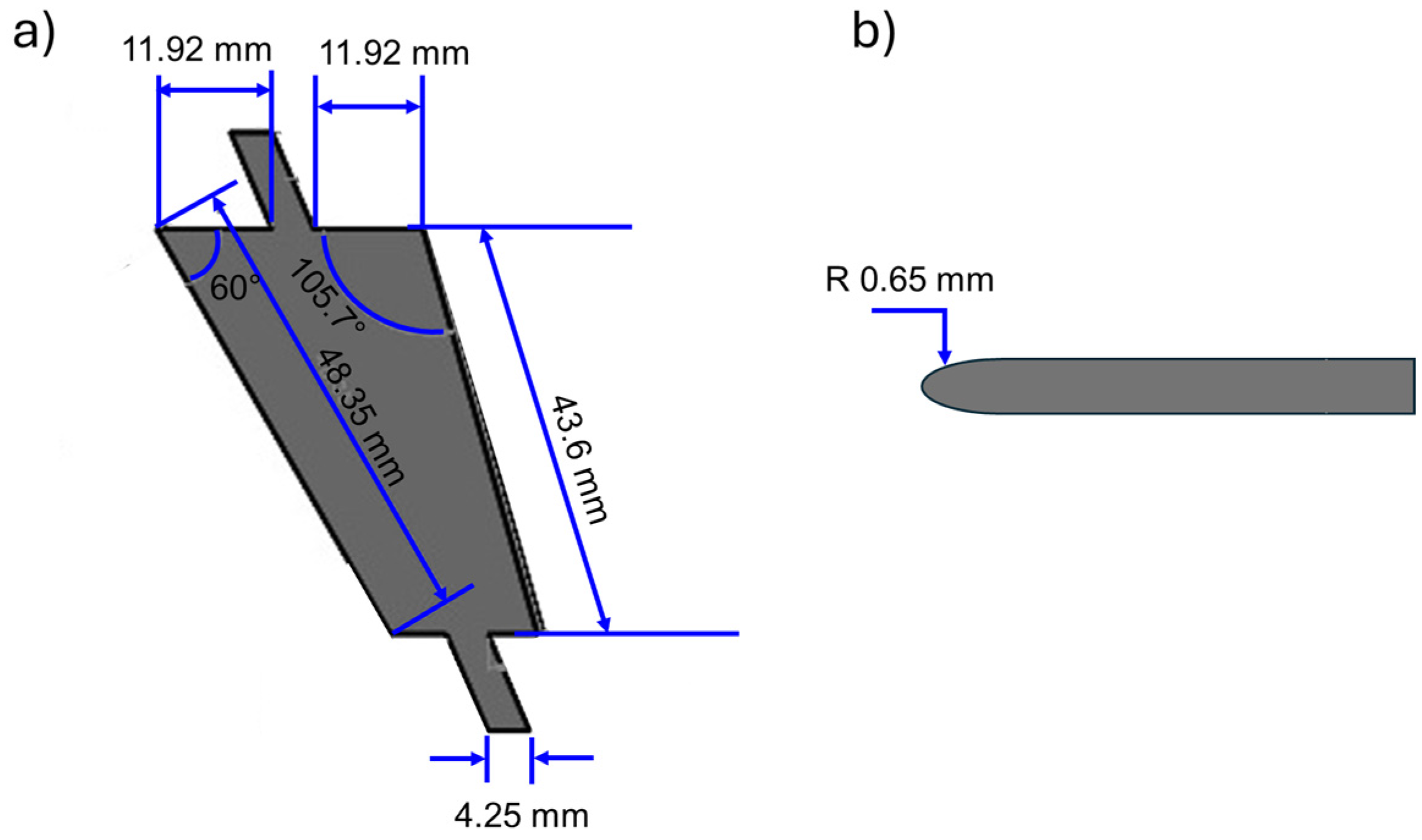
A 65 mm × 40 mm × 0.65 mm (length, width, and thickness) sample of AA 2024-T3 (Al-4.24C-4.46Cu-1.26Mg-0.65Mn-0.15Fe-0.06Si-0.08Zn-0.03Ti in wt.%) was cut through a laser process to produce a trapezoid wing (used in commercial Boing 747 aircrafts) with dimensions indicated in
Figure 1a. Holding appendages (
Figure 1a) were generated with two purposes, fix the wing sample in the corrosion cell and vary the attack angle. The leading edge was ground up to achieve a rounded shape with the dimensions indicated in
Figure 1b. Then, the intrados and extrados surfaces of the trapezoidal wing were also grounded with sandpaper with 2000 grit and polished with microcloth and colloidal alumina of 0.2 μm.
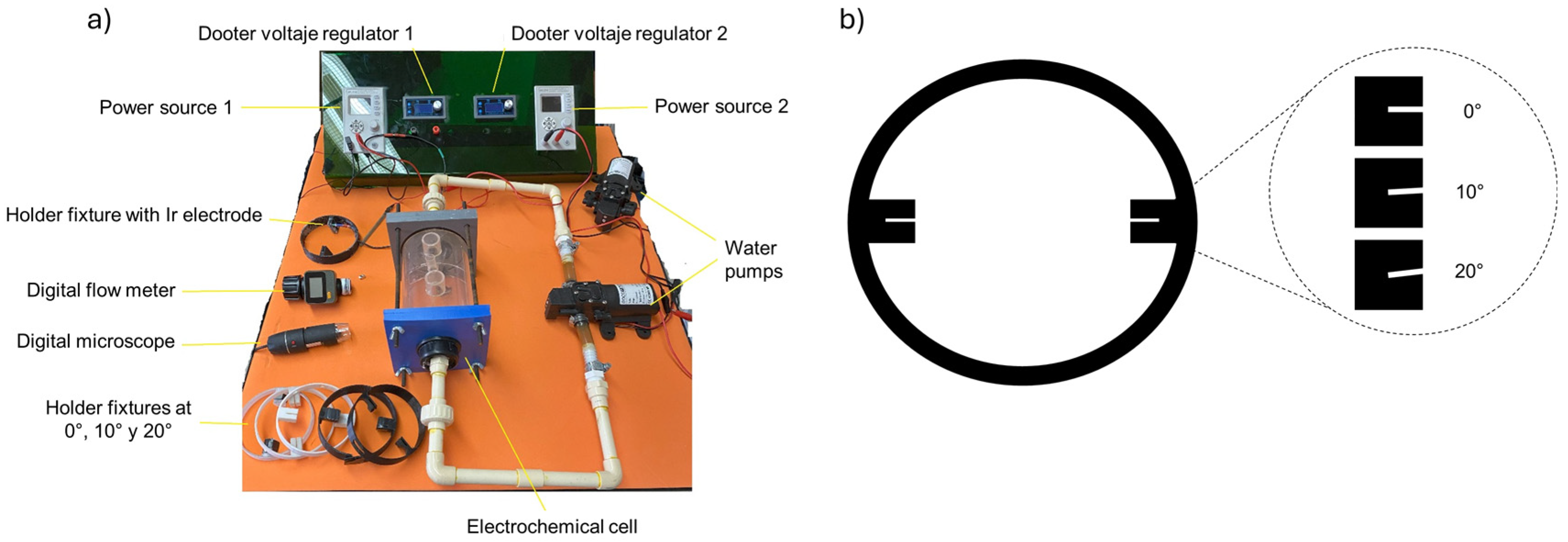
Figure 2 shows the dynamic corrosion cell built to induce pitting degradation in the trapezoid wing samples (
Figure 1a). The experiment considered the variation of the following parameters: attack angle, saline concentration, and electrolyte flow velocity. A stainless-steel grade 304L electrode was introduced through the upper nozzles, which acted as a cathode. Also, a wire connected to an iridium terminal (anode) was introduced into the cell. The anode was fixed to a 3D-printed nylon holder, as shown in
Figure 2b. At the same time, the holder fixture was used to vary the wing attack angle. The electrolyte flow velocity was regulated by employing a variable power source and modifying the voltage provided to the water pump. The magnitude of the flow velocity was measured with a digital flow meter placed in the pipe inlet, as indicated in
Figure 2a.
The current intensity applied to the iridium terminal (anode) in all tests was 0.02 A. This current level increased the corrosion rate in the AA 2024-T3 samples and generated surface degradation once the pitting potential (
) breaks the protective passive layer [
19]. In addition, the pitting degradation was accelerated by the electrolyte mobility (saline solution) and the overpotential level provided since considerable defects can be detected in three hours.
After each dynamic corrosion test, the sample was washed with distilled water and dried with hot air to remove the remaining saline solution. Later, the sample was weighed with a digital scale (sensitivity of 0.01 g). Prior to the dynamic corrosion test, the roughness of polished wing samples was measured in three scans parallel to the span line. Then, the degraded wing roughness was also measured to locate the regions with higher defect accumulation. The surface area of the corroded region was measured using micrographs processing taken with the light optical microscope (LOM) Optika® (Bergamo, Italy). Each corroded specimen was examined utilizing macro and micrographs in the leading edge and the intrados/extrados surfaces using LOM. Up to 30 random micrographs were analyzed. At least 20–30 pits were measured to determine an average defect size by experiment.
The region with high pitting accumulation (located in intrados or extrados) was grounded with 2000-grit sandpaper to remove material (up to 0.01 mm). The material loss was measured with a digital flat spindle tip micrometer. Every 0.01 mm micrograph was taken at 50×. The grounding process continued up to the pits disappearing from the surface. Finally, the deepest defects micrographs were processed with Image J® 1.51p to generate a pit 3D image.
2.1. Orthogonal L9 Design of Experiments (DoE)
The effect of flow velocity, electrolyte NaCl concentration, and attack angle parameters on the pit length and the degraded area during the dynamic corrosion test in the trapezoidal AA 2024-T3 wing sample was analyzed through a DoE based on the Taguchi method [
23]. In this case, an orthogonal design L9 (three parameters at three levels) was employed, as indicated in
Table 1.
The values assigned to the attack angle (0°, 10°, and 20°) promote a significant variation in the stability and boundary layer separation in the wing, as observed in [
24]. In addition, the maximum lift occurred at an attack angle between 15° and 20° [
25]. The NaCl solution concentrations were selected to induce average-to-high pitting corrosion levels in a short time-lapse (3 h). The applied flow velocities maintain a fully developed laminar regimen at the cell inlet.
The quality characteristic “the-higher-the-better” was applied to the DoE to identify the operating conditions (
Table 1) that promote the formation of bigger corrosion pits (in length and depth). The mean-square deviation (MSD) for the selected quality characteristic was calculated through Equation (1).
where
D represents the magnitude of the response variable (pit length/degraded area) measured in the experiment. The signal-to-noise (
S/N) relationship was obtained to measure the desirable quality characteristic deviation. Equation (2) served to calculate the
S/N ratio according to the quality characteristic.
The analysis of variance (ANOVA) was carried out using the
S/N ratio to determine the parameter levels with a higher contribution to the variation in the quality characteristic. For this purpose, Fisher’s F test was used [
26].
2.2. Potentiodynamic Polarization Test
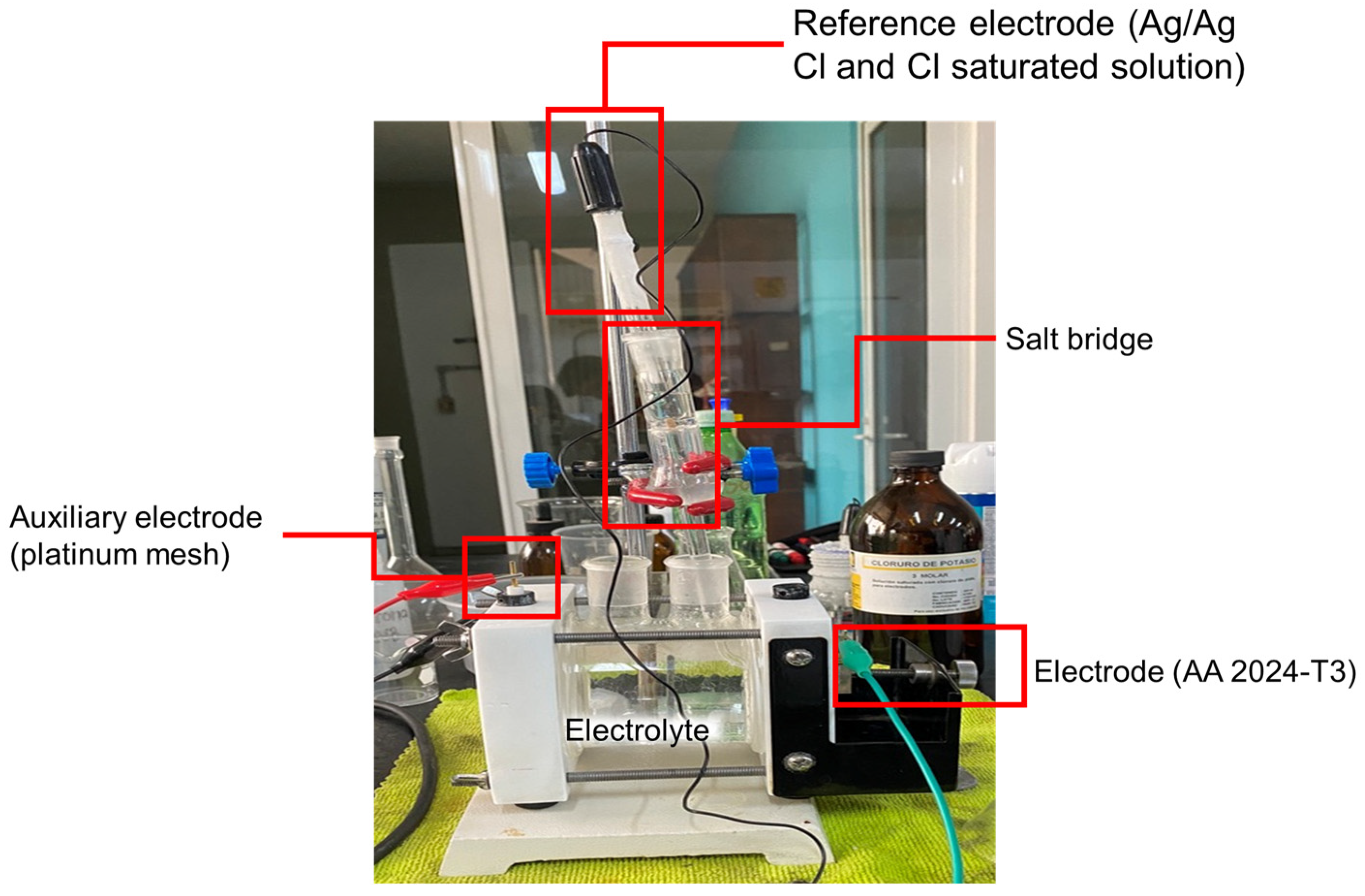
The open-circuit potential (OCP) technique was used to analyze the corrosion behavior of AA 2024-T3 specimens with a 1 cm
2 exposed area varying the saline concentration. The electrochemical tests were performed in the CorrTest Electrochemical Workstation CS350 with the configuration shown in
Figure 3. The main components of the corrosion cell (
Figure 3) were: (a) electrode (AA 2024-T3 specimen), (b) auxiliary electrode (platinum mesh), (c) reference electrode (Ag/Ag Cl and Cl saturated solution), (d) salt bridge, and (e) electrolyte (saline solutions). The electrochemical impedance spectroscopy tests allowed us to measure the corrosion rate, current and corrosion potential, as well as identify the type of corrosion process. The saline solutions at 2.5 wt.%, 3.5 wt.%, and 4.5 wt.% NaCl were prepared using distilled water, analytical balance, a volumetric flask, and a stirring rod.
2.3. Numerical FV Model
The flow velocity distribution, shear stresses, and the separation point of the boundary layer were estimated through the numerical solution of continuity (Equation (3)) and momentum (Equation (4)) equations.
where
represents the electrolyte density (saline solution),
is the flow velocity vector,
the pressure, and
the viscous shear stresses. Considerations applied to the mathematical model were the following:
The mathematical model (Equations (3) and (4)) was simplified to a bi-dimensional (2D) steady-state system considering the fully developed laminar flow that arrives at the wing specimen.
The saline solution was considered as a Newtonian and incompressible flow.
The flow properties of the saline solution were constant and taken from the literature (see
Table 2).
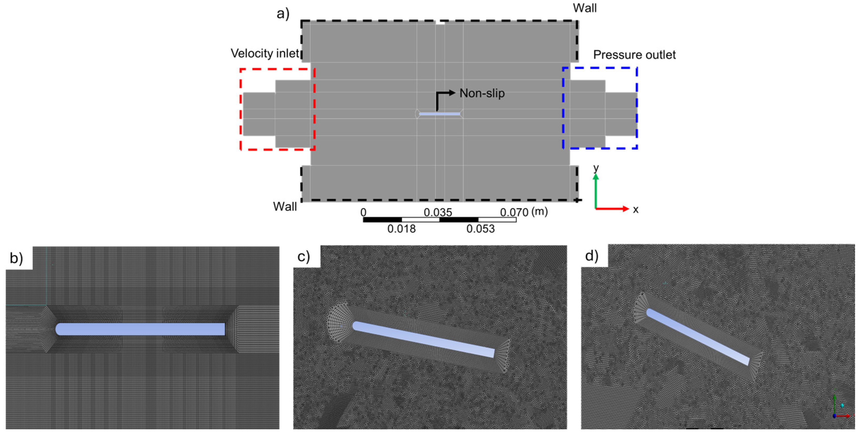
The finite volume model (FVM) was solved numerically by applying boundary conditions such as inlet velocity, pressure outlet, and wall indicated schematically in
Figure 4. The coupled scheme was employed to solve simultaneously the pressure-velocity coupling.
Figure 4b–d show the finite volume mesh used to subdivide the 2D calculation domain. This mesh is comprised of quad and tetrahedron volume types with a quality mesh of 0.85 and a low skewness (0.05), which indicates good mesh quality. Note that a mesh refinement close to the wing surface (
Figure 4b) was applied to improve the numerical estimation accuracy in the boundary layer and its behavior (velocity field). At a distance of 150 mm, a coarse mesh was applied to reduce the number of volumes and the computing time.
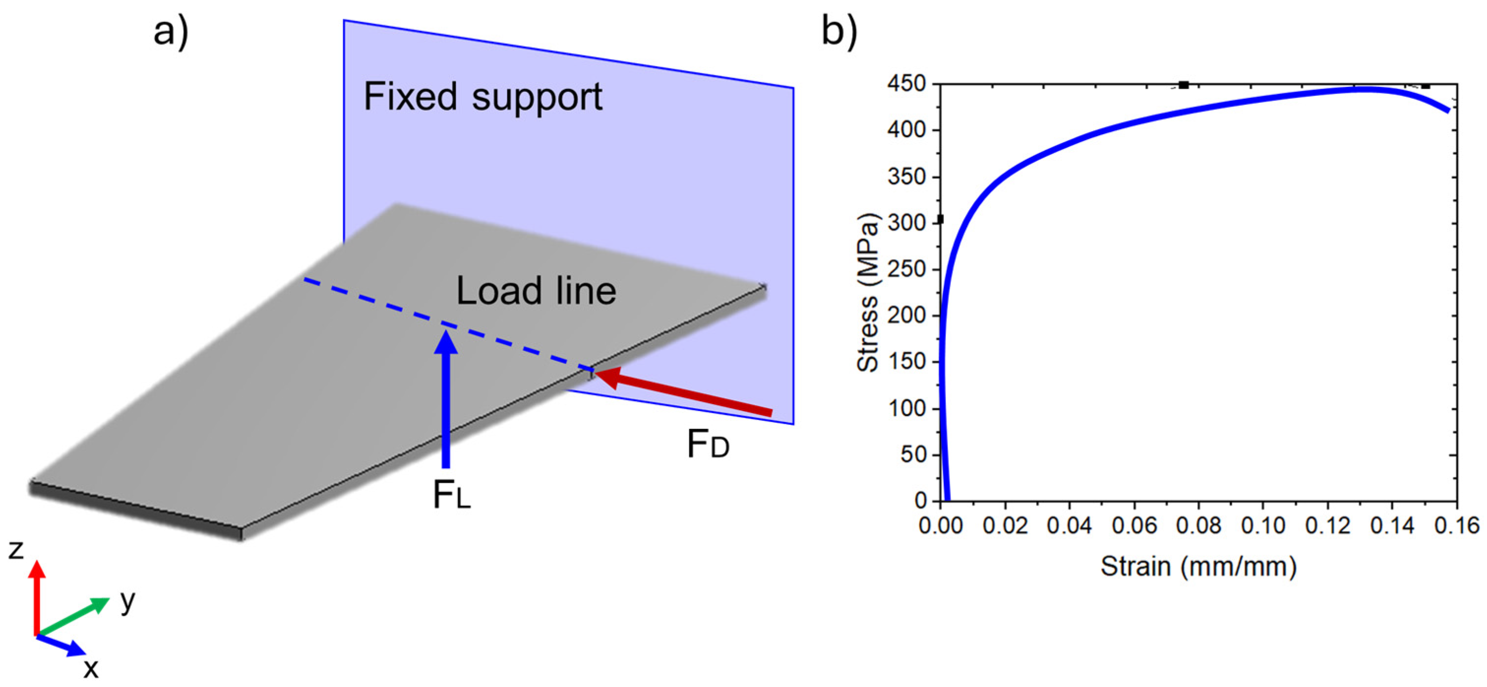
2.4. FE Model
A finite element (FE) model was employed to solve numerically the steady state bending equation (Equation (5)), which allowed us to estimate the deflection and slope distributions caused by the alternate application of drag (F
D) and lift (F
L) forces. The main considerations are listed as follows:
Only punctual lift (
) and drag (
) forces were applied in the wing center of pressure as indicated schematically in
Figure 5a.
Firstly, the lift (
) and drag (
) coefficients were estimated at different attack angles 0–20°, varying the Re number between 10,000 and 18,000. The drag and lift forces were calculated through the plant area
(span chord line),
and
coefficients, as well as the inlet fluid flow velocity (
) as indicated in Equations (6) and (7).
The support between the wing and the fuselage was defined as a fixed support, restricting deflection and slope (
Figure 5a)
The fatigue analysis applied the Goodman criterion to estimate fatigue life and safety factor. Mechanical properties such as the Young modulus (
), yield strength (
), ultimate strength (
), and fatigue limit (
) were extracted from the engineering stress–strain diagram of AA 2024-T3 shown in
Figure 5b. In zones with high degradation by forming and accumulating critical pits (most extensive), resultant defects were obtained. The high degradation zones were those regions in extrados/intrados where the roughness was higher than 0.59 μm. Critical pits were defined considering their maximum depth and morphology revealed with the LOM analysis. These defects were introduced into the AA 2024-T3 wing as “frozen bodies”. These punctual defects were located at the high normal stress region. To simulate the material loss, the mechanical strength assigned to the frozen bodies was negligible (E = 0.001 GPa).
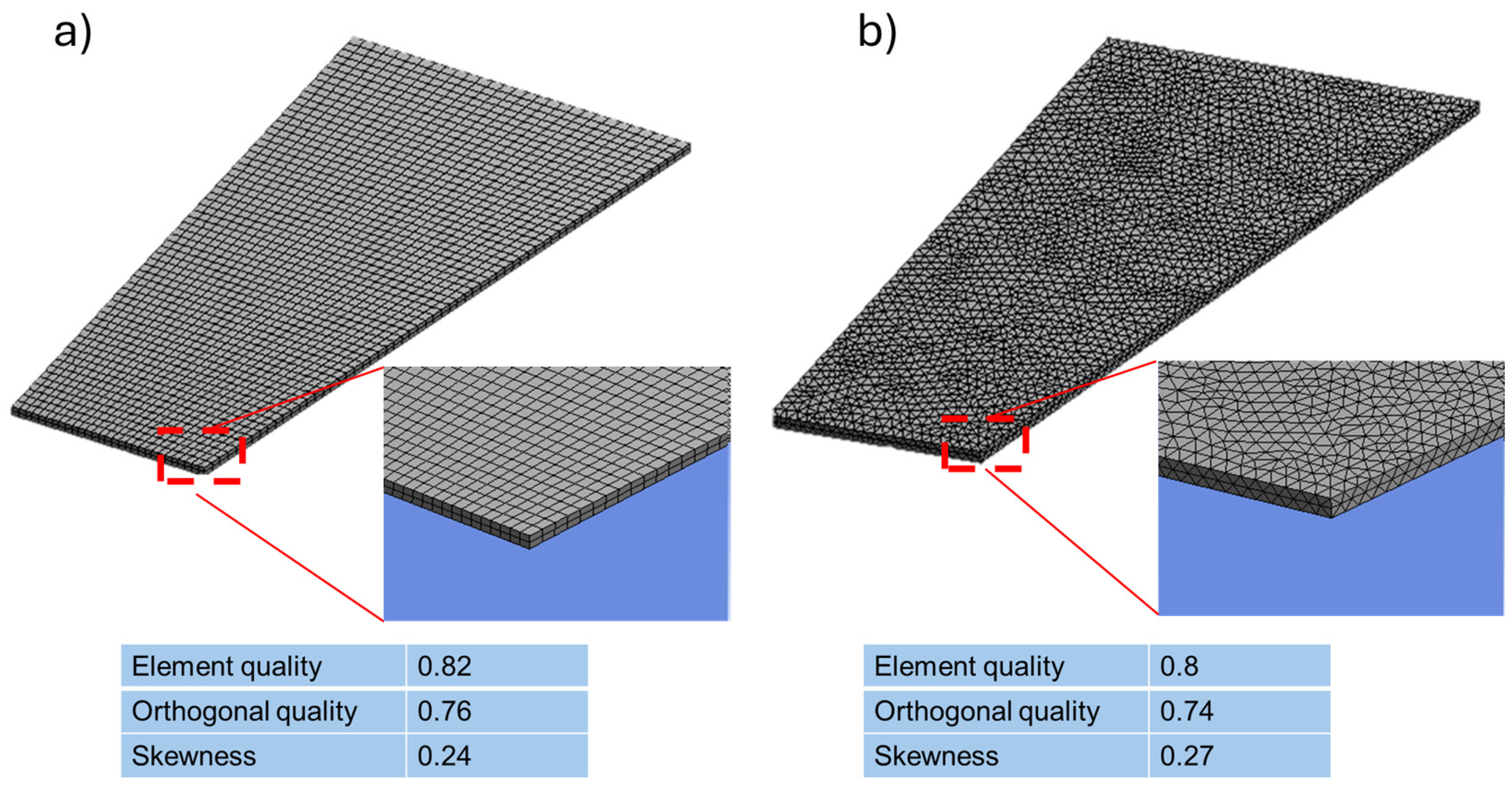
Figure 6a,b show the FE meshes of hexahedral (20 nodes) and tetrahedral (10 nodes) high-order elements employed to subdivide the wing without defects and after adding frozen bodies (critical pits). Mesh refinement was applied in regions near the added defects employing face sectioning. The average mesh metrics element quality, orthogonal quality, and skewness indicated a good quality.
3. Results
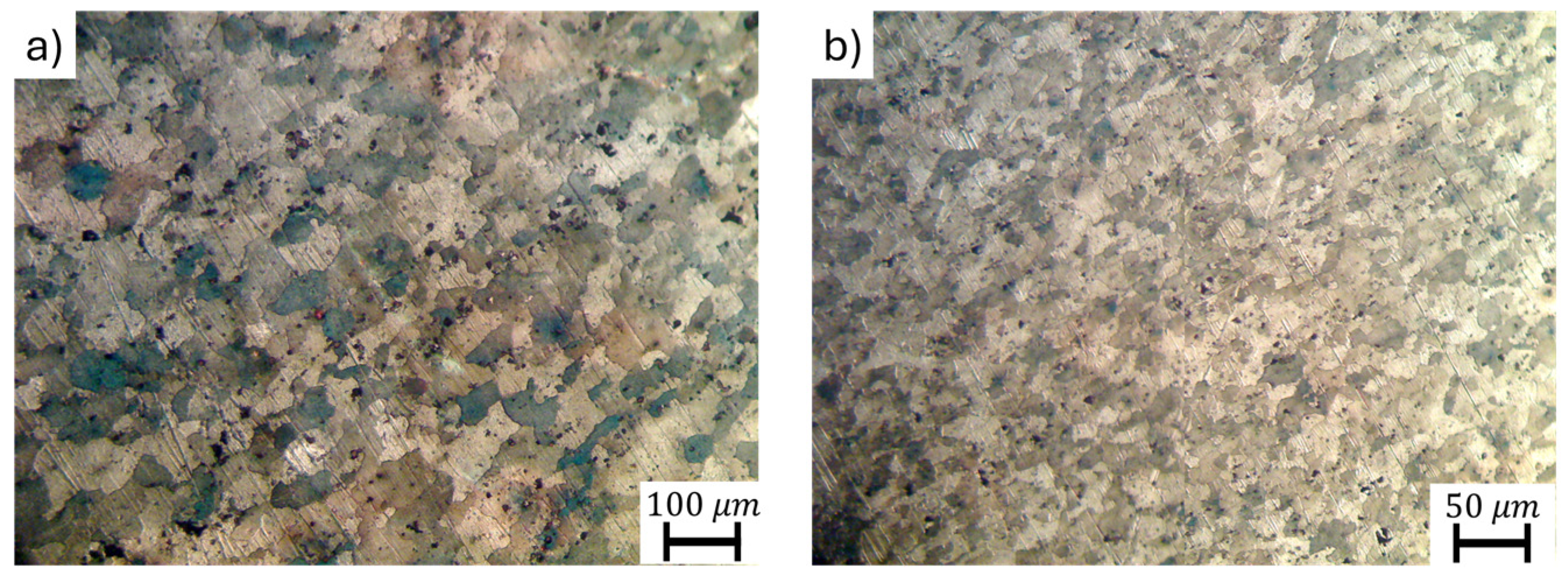
AA 2024-T3 exhibited a granular microstructure, as shown in
Figure 7. Representative LOM micrographs taken from the extrados region indicated a homogenous grain size distribution mainly composed of an average grain size of 67 ± 5 μm.
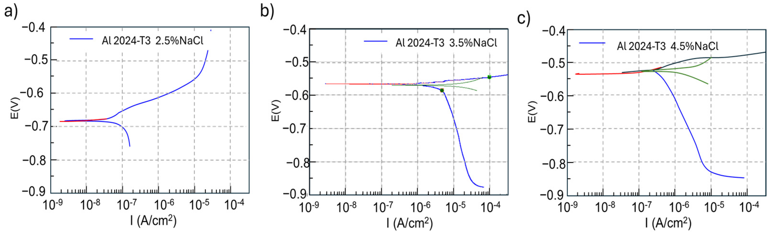
The potentiodynamic curves of polarization resistance in
Figure 8 were obtained in static conditions. Corrosion potentials of −0.72, −0.57 and −0.54 were obtained for saline concentrations of 2.5%, 3.5% and 4.5% wt. NaCl, respectively. In
Figure 8, the red line represents the linear polarization resistance curve and the green line indicates a projection of this curve. A surface passivate oxide layer was formed in all cases, which increased the AA 2024-T3 corrosion resistance.
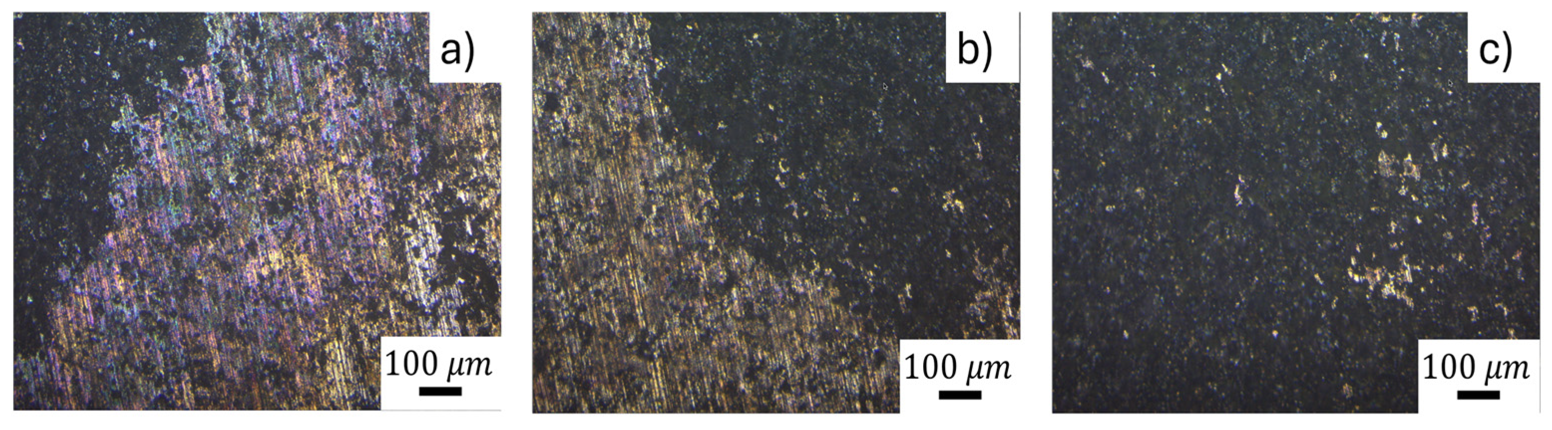
The surface degradation caused by the saline solution changed proportionally with the NaCl concentration, which was corroborated through the affected area. The percentages of the degraded area were obtained by comparing the free defects area against the corroded one in each sample. Degraded area percentages of 48.2%, 57.7%, and 70.6% were measured for the three saline concentrations.
Figure 9 shows representative LOM micrographs of the surface degradation caused by the static electrochemical test in the AA 2024-T3. As was mentioned before, pitting clusters were formed when the NaCl concentration increased (
Figure 9a–c), giving rise to the formation of prominent degraded regions (dark zones,
Figure 9c) and regions with isolated pits (
Figure 9a,b). Pits had circular and elliptical morphologies. Although, some pits were amorphous (
Figure 9a,b).
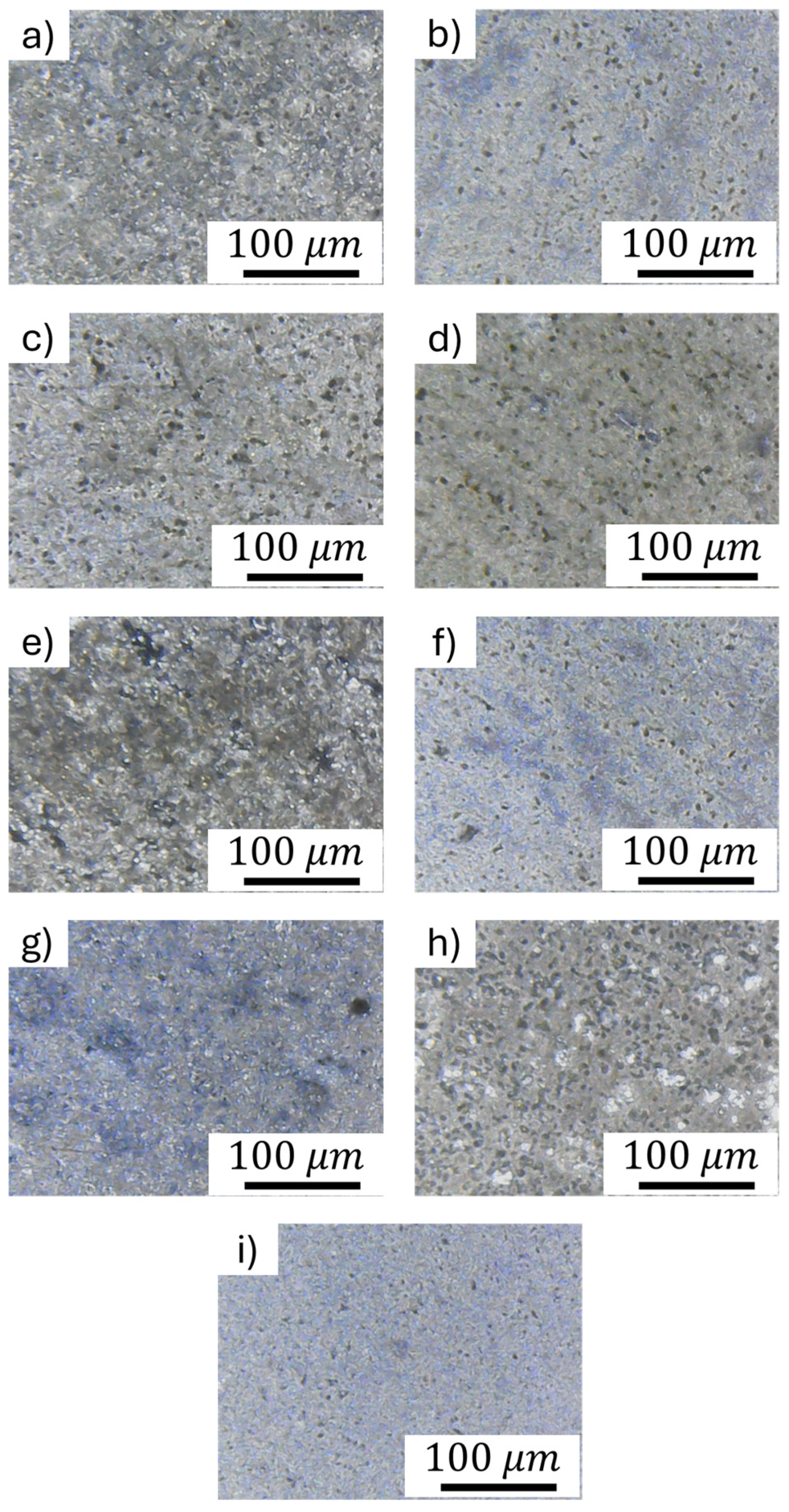
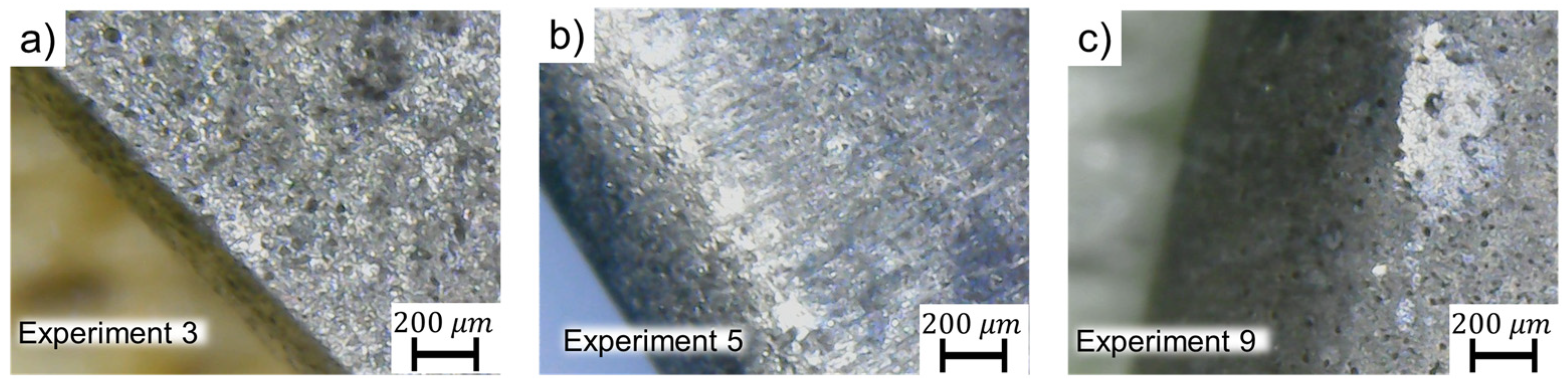
On the other hand, the pits morphology and their distribution observed during the dynamic electrochemical test in the wing specimens changed considerably.
Figure 10 and
Figure 11 show micrographs taken from representative regions (with high degradation) in intrados and extrados of each experimental condition (
Table 1). As can be seen, the corrosion induced dynamically caused also pits with circular and elliptic morphologies (
Figure 10a,d and
Figure 11a–d) but with an increment in the number of elongated-amorphous pits in intrados (
Figure 10e–i) and extrados (
Figure 11e–i). It is worth mentioning that the formation of pits clusters is characteristic of degradation caused by the static corrosion. Therefore, this effect occurred less frequently under dynamic conditions (see
Figure 10 and
Figure 11). Only test 5 exhibited many pit clusters in intrados (
Figure 10e) and extrados (
Figure 11e), which gave rise to extended degraded regions. Tests 4 and 6 also showed some pit clusters, as shown in
Figure 10d,f and
Figure 11d,f but were lower than test 5.
Table 3 resumes the main metrics (pit length and degraded area) obtained from the micrographs of degraded surfaces (up to 30 random fields by specimen).
The average pit length was similar in extrados and intrados regions for all experiments (
Table 3), corroborating with the low calculated standard deviation. As was expected, tests 4–6 had the higher standard deviations derived from the pits clusters that induced the formation of amorphous degraded zones. On the contrary, the percentage of degraded area (
) in all cases was higher in the intrados region (
Table 3). Tests 4 and 8 even exhibited 50% higher degraded areas in the intrados than in the extrados region (
Table 3).
According to
Table 3, tests 5–6 had the average biggest pit length (0.181 mm and 0.176 mm) in the extrados region. Nonetheless, the higher (
was measured in test 8 (11.18%), where the pitting formation was massive in both intrados (
Figure 10h) and extrados (
Figure 11h). Although, the number of pits clusters was lower than the tests 4–6. Meanwhile, test 7 had the lower average pit length (
, extrados) and
(1.35%, extrados). Tests 1–3 performed without attack angle (0°) and presented similar average pit length magnitudes. This highlights the high
in extrados and intrados with the NaCl concentration increment. The
in test 3 (6.05%, intrados) reached double compared to test 1 (3.05%, intrados), which also was notorious in the degraded surfaces (
Figure 10a,c).
A more detailed analysis of the effect of attack angle, electrolyte saline concentration, and flow velocity parameters on the pit length and
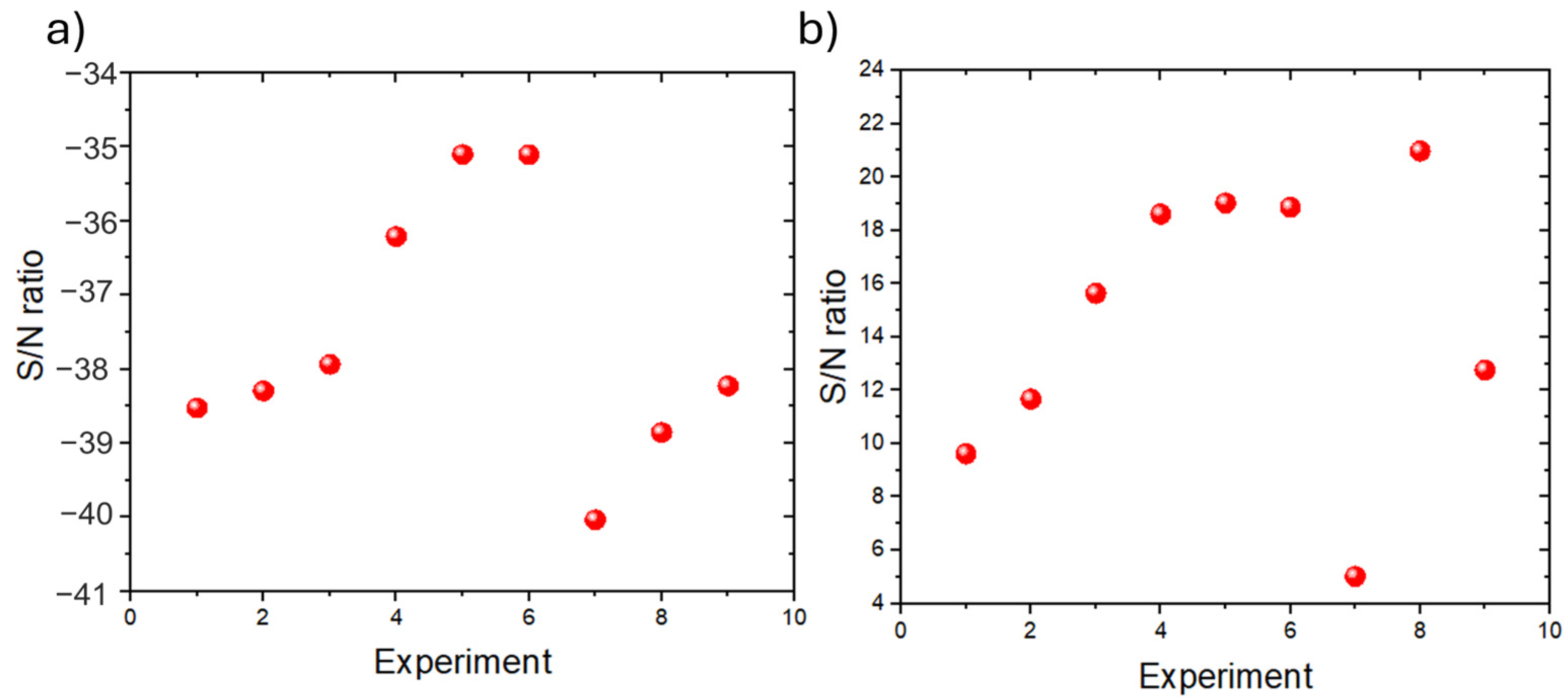
was carried out with the DoE Taguchi. In this case, the aim was to determine the combination of the optimal parameters to increase the pit length and
identify the main parameters for each response variable. The MSD (Equation (1)) and the S/N ratio (Equation (2)) calculations employing average pit length and
are resumed in
Table 4. Then, the S/N ratio results allowed us to generate ANOVAs shown in
Table 5 and
Table 6.
Fisher’s F test helped identify the most significant parameter statistically (
) [
26] for each response variable, considering a significance level of 95%. According to the ANOVA of
Table 5 and
Table 6, any parameter was statistically significant (
). However, in both cases, the attack angle had the higher contribution for the pit length (up to 90%) and the
(49.9%).
Figure 12 shows graphically the S/N ratio distribution for each response variable according to the parameter’s levels. From these graphs, it was deduced that the parameters configurations A2B3C1 and A2B2C1 promote the higher magnitudes for pit length and
, respectively. Both cases coincide with the attack angle (10°) and the lower flow velocity (2.85 lt/min) to induce higher corrosion degradation in the wing skin. Nevertheless, it must be recognized that the electrolyte saline concentration has a higher contribution than the flow velocity and changes for both response variables.
In order to complement the morphology analysis and critical pit size, all corroded samples were grounded in extrados and intrados to reduce the thickness to 0.01 mm from the surface. Several pits disappeared after the ground level reached 0.05 mm, which occurred in tests 1 and 7 (see
Figure 10a,g). While most pits in the other samples disappeared in a range between 0.07 and 0.09 mm. On the other hand, the deepest pits were detected in test 5 (0.11 mm) and 8 (0.14 mm). The deepest pit morphology in tests 5 and 8 was elliptical and, in both cases, was located behind the leading edge, in the zone next to the fuselage (fixed region).
3.1. CFD Results
The fluid flow field developed around the wing under the three orientations (0°, 10°, and 20°), and the varying Re number in the range10 × 10
3–18 × 10
3 was estimated by means of the CFD model.
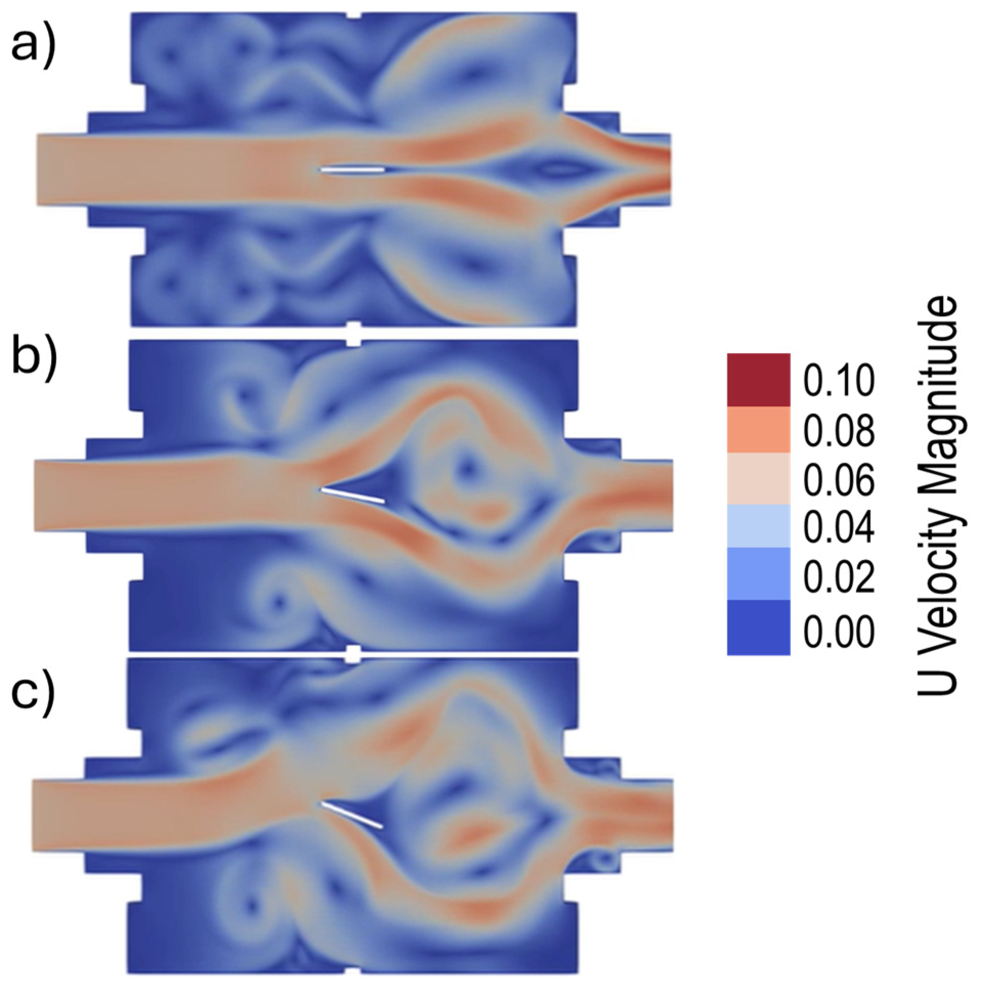
Figure 13 presents the estimations of flow velocity distribution and its behavior once the flow field is stabilized.
According to the CFD estimations of
Figure 13a, the velocity remained constant in the wing boundary layer without attack angle (0°) in both intrados and extrados due to the negligible perturbation. Nevertheless, the boundary layer behavior changed for the wings with other attack angles (10° and 20°). For instance, the wing with an angle attack of 10° stayed attached to its boundary layer for almost all the chord line on the intrados side, as displayed in
Figure 13b. In the wing with an angle attack of 20°, the boundary layer stayed attached up to ¾ of the chord line length (
Figure 13c). On the contrary, the separation of the boundary layer in the extrados surface occurred after the leading edge in both cases (
Figure 13b,c). As was expected, flow velocities were higher with the Re number increment.
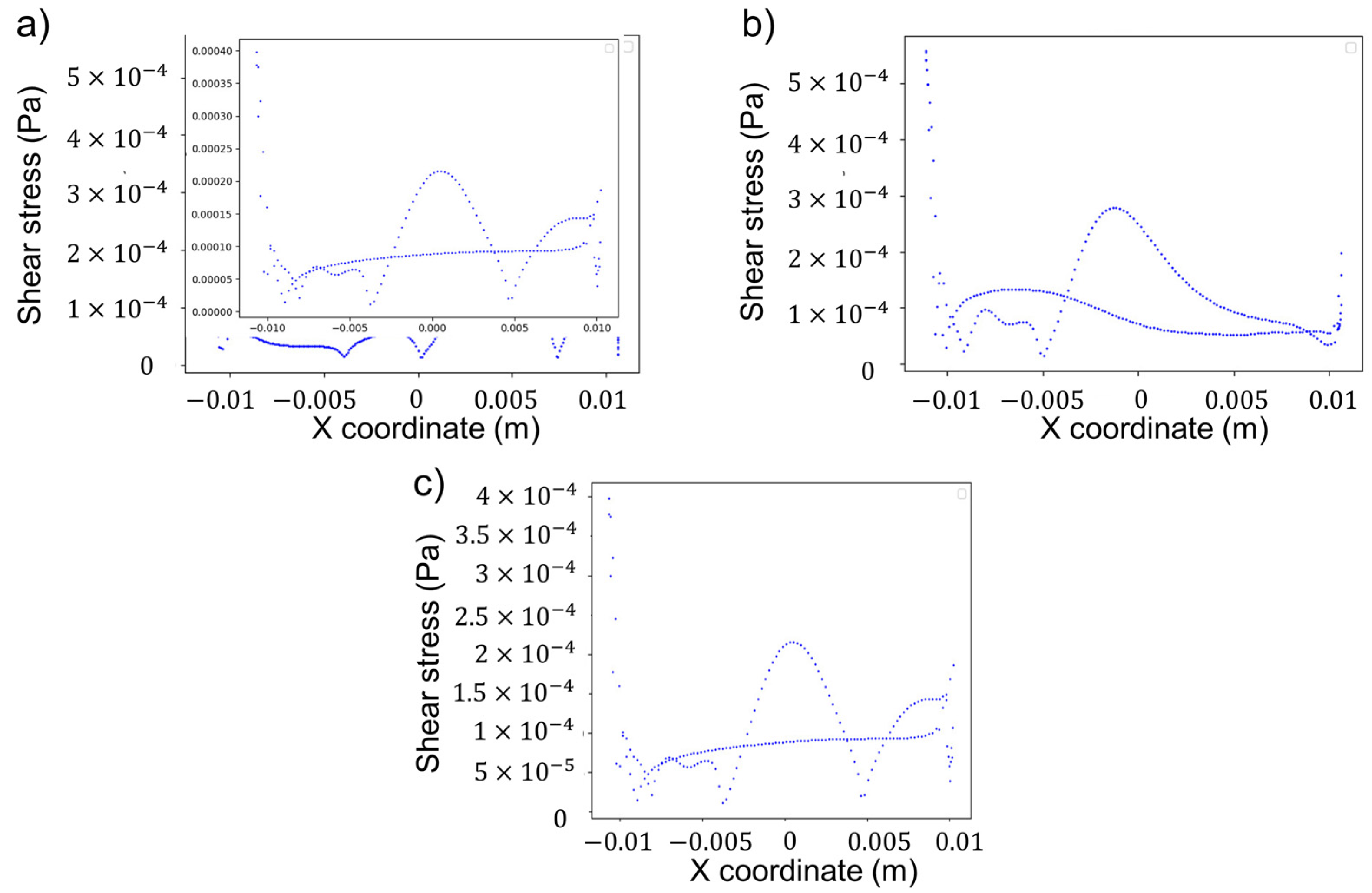
The viscous shear stresses estimations also were uniform in all chord line lengths for the wing without attack angle (
Figure 14a) and only increased with the flow velocity. Meanwhile, the shear stresses were only significant for the intrados region in the wing with attack angles of 10° (
Figure 14b) and 20° (
Figure 14c). In
Figure 14, the “x coordinate” represents the horizontal position of each cell center along the wing’s surface, while the “shear stress” was calculated using Newton’s law of viscosity. Each plot depicts the shear stress on the wing’s upper (suction side) and lower (pressure side) surfaces. The magnitudes are low due to the no-slip condition at the walls and the low-velocity field within the boundary layer. Higher shear stress values are observed primarily near the leading edge where the flow impacts the wing, resulting in steeper velocity gradients. On the lower side, the shear stress distribution is more uniform along the wing. While on the upper side, peaks are evident, especially at higher angles of attack, due to boundary layer separation.
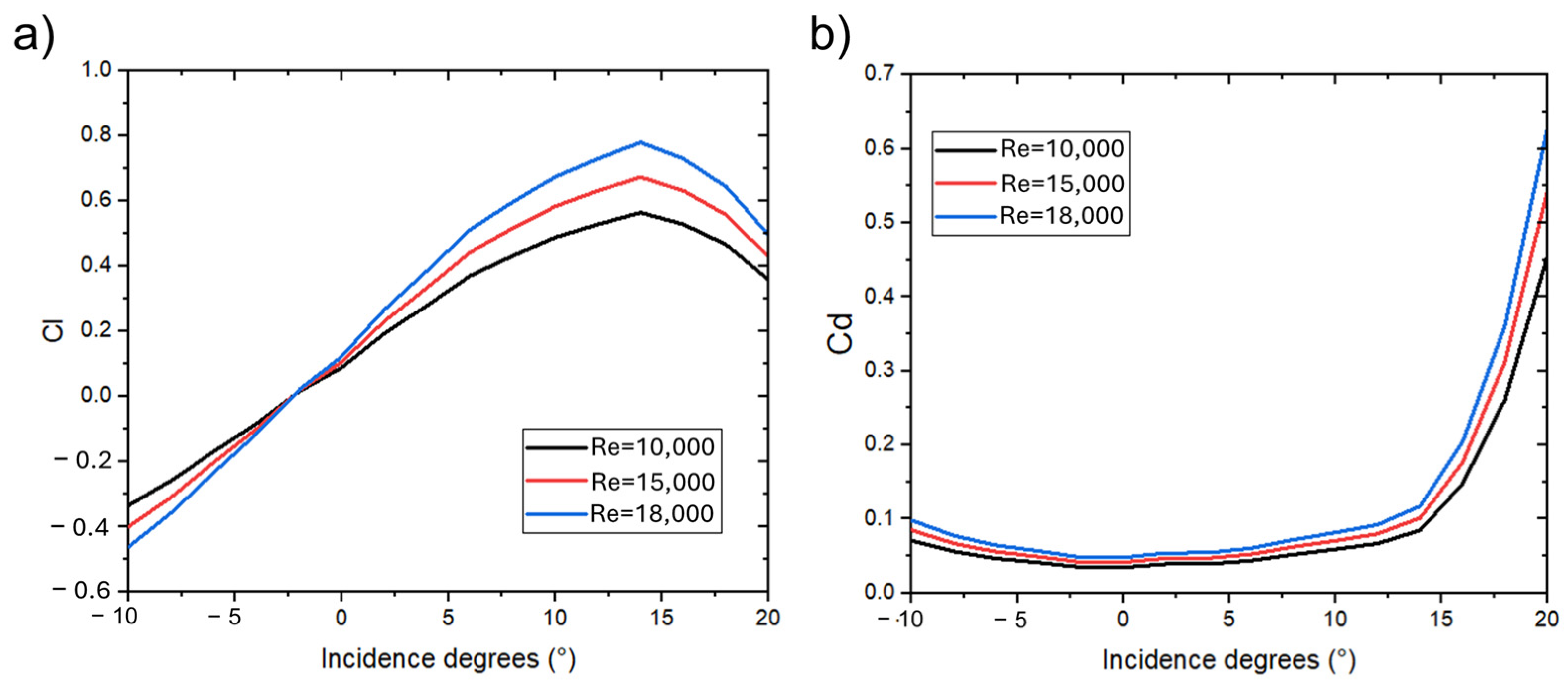
The performance wing metrics and the drag and lift coefficients were also estimated considering the wing orientation (attack angle) and the Re number magnitude. Graphs of
Figure 15 show the estimated C
l and C
d magnitudes, respectively.
3.2. FEM Results
Through the C
d (
Figure 15a) and C
l (
Figure 15b) coefficients estimated numerically, the lift (Equation (6)) and drag (Equation (7)) forces were calculated and introduced into the FE model as natural boundary conditions. Graphs of
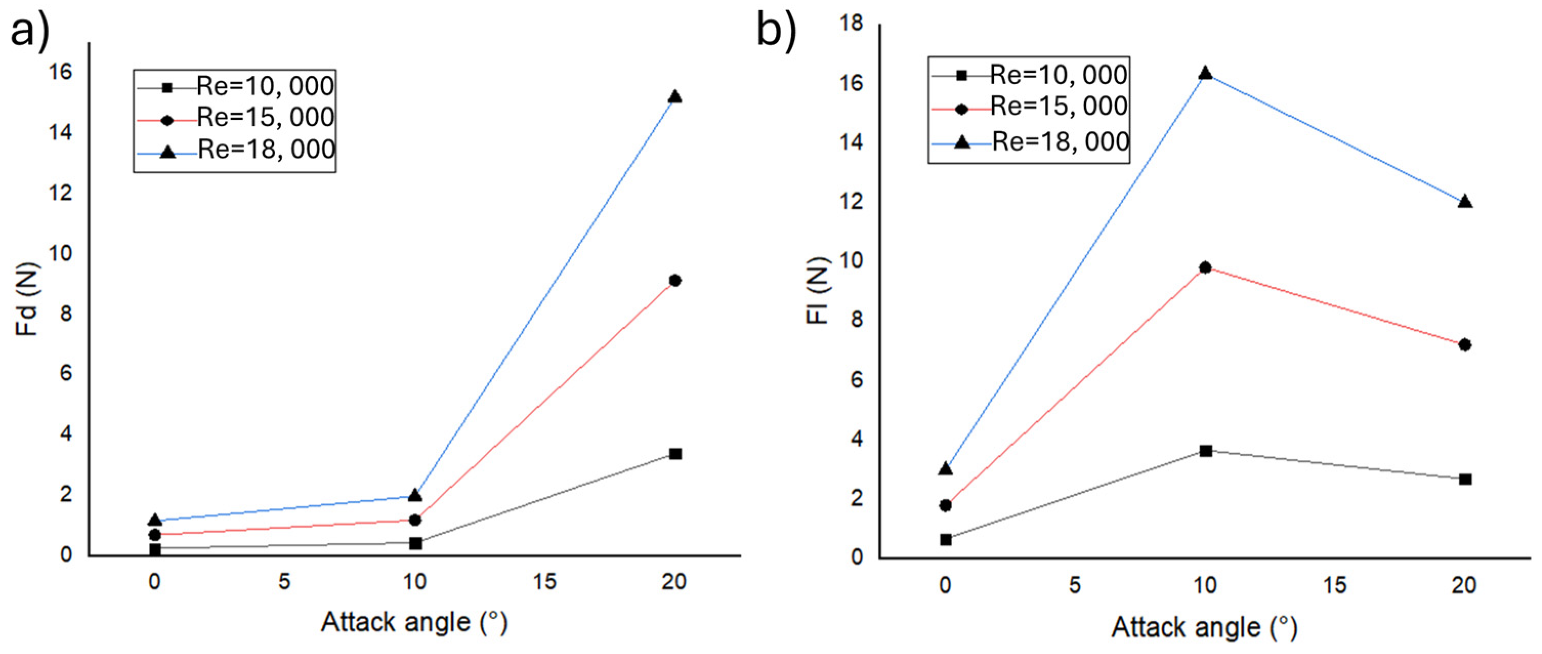
Figure 16 show the magnitudes calculated for drag (
Figure 16a) and lift (
Figure 16b) forces considering the attack angle and Re number variations.
Figure 17 indicates the normal stress (
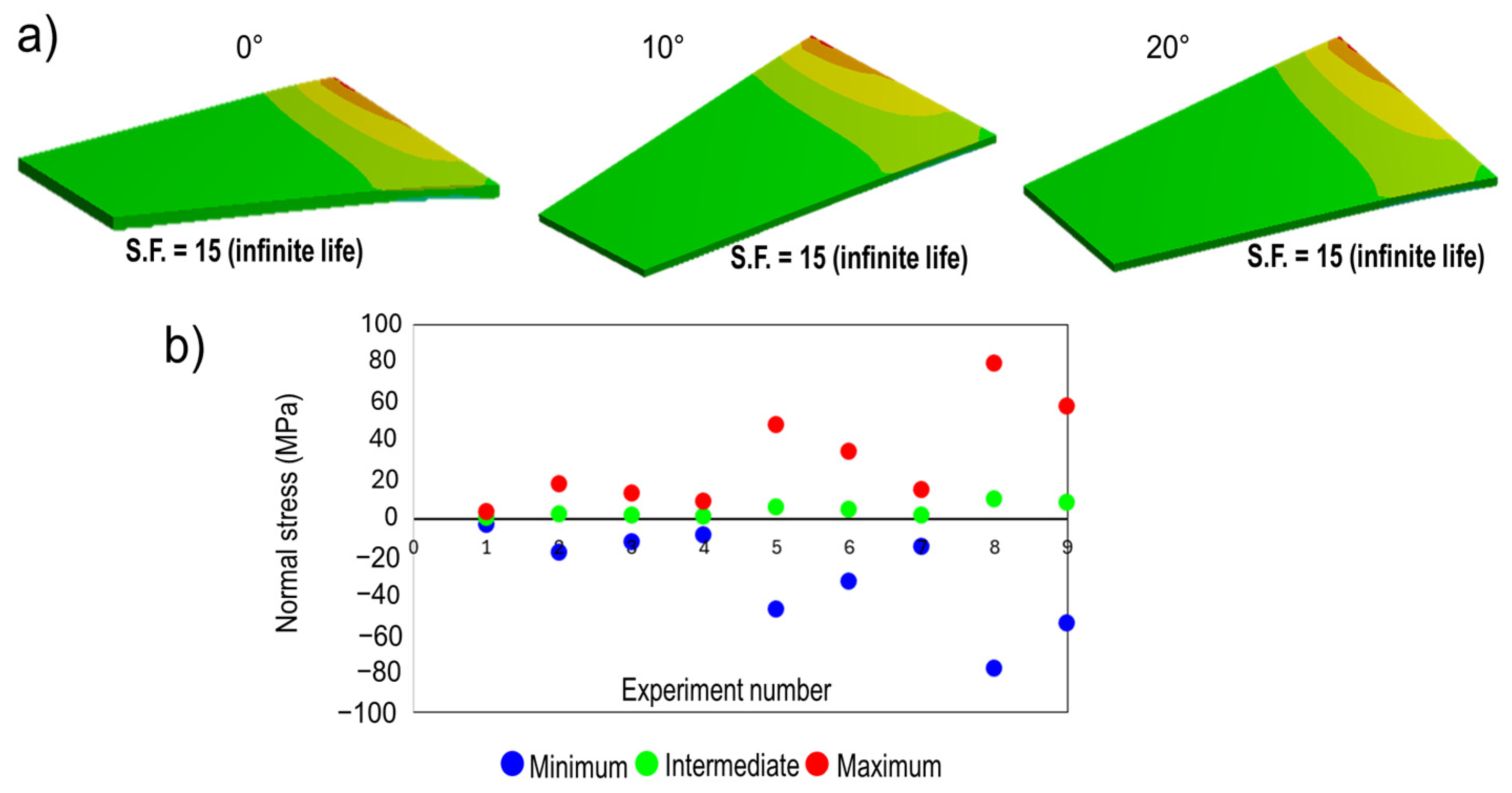
) distribution caused by the lift force, which tends to produce a higher deformation (deflection) effect since this force acts on the wingspan. For the three Re numbers assessed, the maximum stresses were produced at an attack angle of 10° (
Figure 17b). Correspondingly, the maximum deflection was estimated for this attack angle (10°), varying the Re number, as can be seen in
Figure 17.
Due to the low magnitude of the drag and lift forces (
Figure 16) induced by the flow conditions, all cases of the FE model predicted infinity life with a high fatigue safety factor (SF), up to 15 (see
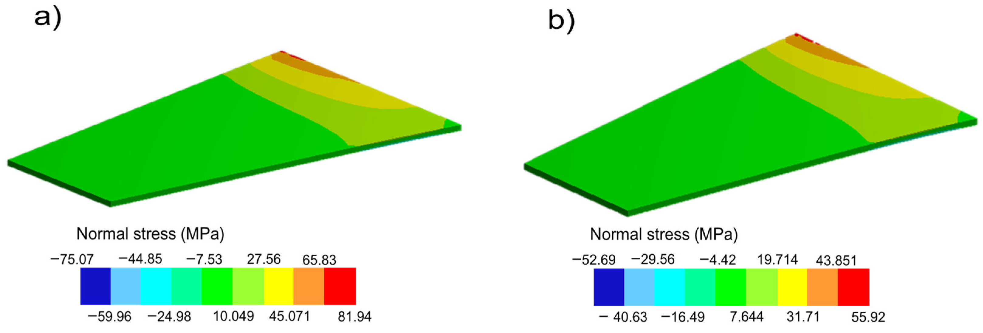
Figure 17). Nonetheless, the fatigue SF fell up to 6.67 in the case of the wing with an attack angle of 20° for a Re of 18,000, producing a maximum normal stress of 57.83 MPa (test 9,
Figure 17b). Thus, critical size pits along with a high normal stress level in the region close to the fuselage can give rise to the formation of microcracks and cracks responsible for the fatigue failure. In order to evaluate this possibility, fatigue wing performance with elliptical defect concentration (largest pits) was simulated.
Pits were in the region close to the fuselage where the alternate action of F
l and F
d forces induced the higher normal stresses (
Figure 17b) and lower SF (
Figure 17a). When pits are isolated due to their limited dimensions (even the pits sized 0.02 × 0.14 mm), numerical results predicted a negligible stress increment (
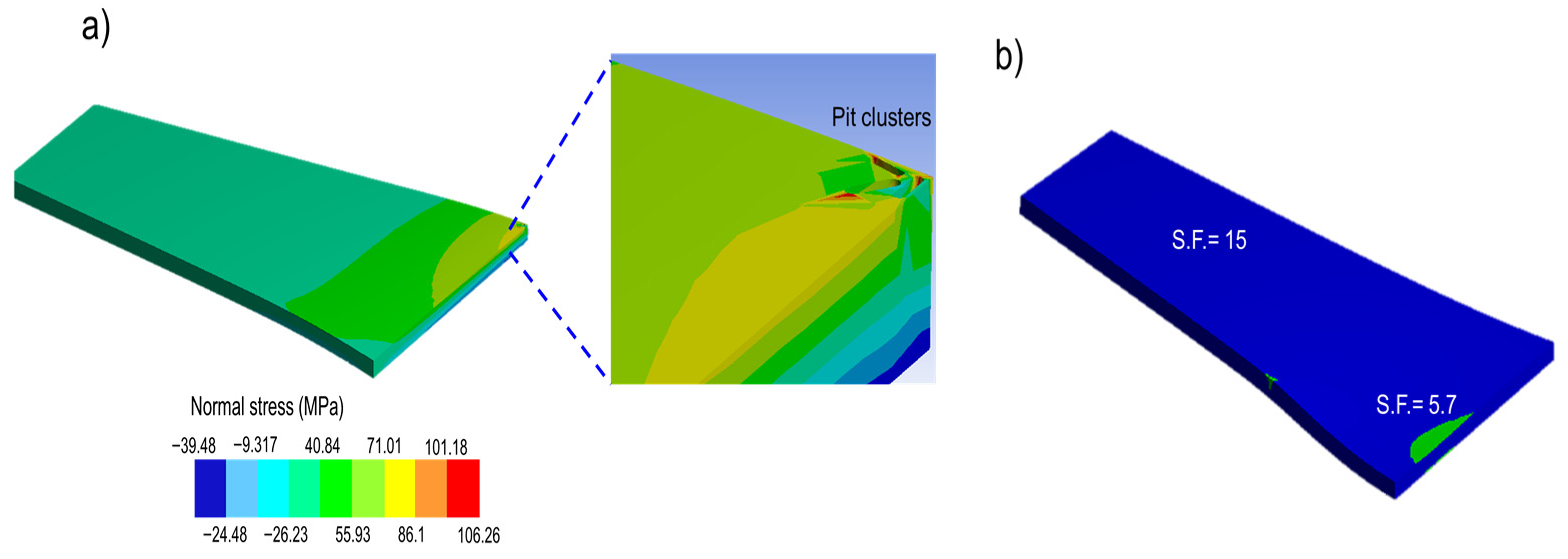
Figure 18a). Rather, pits clusters create the most prominent defects capable of generating stress concentrator sites.
Figure 19a shows the estimations of normal stress around oval defects, representing pit clusters. This highlights the stress concentrators around the defects (
Figure 19a). Depending on the defect orientation and its position, the fatigue SF can suffer a higher reduction, as indicated in
Figure 19b.
4. Discussion
Previously, Duquesnay et al. [
19] and Medina et al. [
28] observed circular, elliptic, and amorphous defects (by pits concatenation) derived from static corrosion test in AA 7075-T6511 and 2024-T3. On the other hand, the electrochemical test with electrolyte mobility (fluid flow) proposed in this research work also caused pits with circular and elliptic morphologies (
Figure 10 and
Figure 11), but with an important increment of amorphous and elongated pits in intrados (
Figure 10) and extrados (
Figure 11). It is known that the formation of the pit is due to the electrochemical reaction that happens among the anode (wing sample) and the cathode (stainless steel bar) when an electrolyte passes between them and allows the electron transport from active to passive zones [
29]. In this case, when the boundary layer was attached to the wing intrados (
Figure 13a), it favored the formation of the pit in this region. Conversely, the flow separation that occurs in the wing extrados with attack angles different of 0° limited the degradation process, as shown in
Figure 11. Additionally, the electrochemical reaction was more effective at low flow velocities (higher electrons interaction between anode and cathode), promoting the larges pit formation. Another important aspect is the high content of Cu (4.46 wt.%) and Mg (1.26 wt.%) in AA 2024-T3, which reduces the intergranular corrosion resistance, as reported by Bałkowiec et al. [
30] and Zhang et al. [
31]. Since the formation of Cu-rich precipitates and intermetallic compounds in grain boundaries (
Figure 7) which act as cathodes, anodic dissolution is promoted, reducing significantly mechanical properties (Sy) and, thus, fatigue strength.
It is worth mentioning that prior to the dynamic electrochemical test, all samples’ extrados and intrados surfaces were polished up to reach a uniform roughness (Ra) magnitude of 0.04 μm to avoid scratches or surface imperfections, which promote passive layer rupture and become a potential site for pits to form form, as reported by [
32].
According to the Taguchi DoE predictions, the largest pits and degraded areas were produced when the tests employed an attack angle of 10°, a NaCl concentration of 3.5% wt., and a flow velocity of 2.85 lt/min (
Figure 12). Additionally, a boundary layer attached to the specimen is required to facilitate the electrochemical reaction, which is achieved at low flow velocities. However, according to the ANOVA, the flow velocity was the parameter with a lower contribution to increasing the corrosion degradation (
Table 5 and
Table 6). On the contrary, contributions of the attack angle (49.9%) and the NaCl concentration (39.5%) were determinants to the creation of zones with higher pitting degradation. The attack angle of 6–10° tends to increase the viscous shear stresses in the airfoil boundary layers, as presented in [
33]. In addition, the attack angle of 10° induced a higher lift force (16.3 N, see
Figure 16b) and, thus, a higher bending moment in the wingspan. In normal operating conditions (without considering the fixed holders in the cell,
Figure 2b), the effect of the higher bending moment during flight conditions can contribute to the passive layer rupture in the AA 2024-T3 and produce the CF phenomenon [
19].
In the dynamic corrosion test, it can be observed that the attack angle of 10° favored a higher interaction between the electrolyte and the specimen retarding the boundary layer separation in intrados higher than ¾ of the chord line length (see
Figure 13b). On the other hand, shear stresses estimations shown in
Figure 14 indicated higher magnitudes with the attack angle increment (up to 20°). A higher shear stress in the hydrodynamic layer indicates a more considerable flow velocity gradient, evidencing a high flow velocity out of the non-slipping region in the wing wall (
Figure 14c). The flow velocity increment caused lower size pits and degraded areas.
The role of the NaCl concentration was key for the adsorption of Cl- ions in the aluminum passive layer with positive charge [
34]. Hence, a higher NaCl concentration in the electrolyte increases the number of pits and their size, which agrees with the DoE Taguchi predictions related to the optimal pit length and degraded area extension (see
Table 5 and
Table 6).
The largest and deepest pits were in the trailing edge region (
Figure 20) and behind this point, towards the assembly region with the fuselage. The stagnation point was produced on the leading edge, which creates favorable conditions for static corrosion degradation (
). Then, the more significant exposure area (next to the assembly region with the fuselage) and the low flow velocities promoted the formation of many pits in the flow velocity recovery zone. Even the formation of pit clusters happened, giving rise to broad degradation zones, as indicated in
Figure 10.
Finally, the FE model evaluated the effect of C
l and C
d coefficients calculated with different Re (10,000, 15,000, and 18,000) and critical pits on the normal stress, deflection, and wing fatigue life. In all cases, the lift force in the fixed support region (next to the fuselage,
Figure 17) produced a higher normal stress due to the wing tip’s high deflection. This stress distribution was correlated with the structural predictions reported by Nguyen et al. [
35] for an airfoil in low-flight speed conditions. The addition of critical-size pits as frozen bodies with negligible mechanical strength (E = 0.001 GPa) in the wing-fuselage assembly region did not change the stress distribution (
Figure 18). Critical pits dimensions (diameter = 0.02 mm, depth = 0.14 mm) did not act as stress concentrators necessary to start a fatigue crack (pre-crack effective size) as informed by [
36]. Therefore, the wing damage was low, the fatigue life was infinite, and the SF remained higher (
Figure 18).
A more critical condition was obtained when pit clusters acted, increasing the defect length and orientation (
Figure 19). Intergranular pits clusters are responsible for reducing significantly mechanical properties (
), and thus, fatigue strength [
31]. When the pit clusters’ effect on fatigue performance was modeled, stress concentration points were generated in the maximum normal stress zones (
Figure 19), reducing the SF. Thus, forming pit clusters is the most critical aspect during corrosion since their proximity and penetration determine when and where the crack will appear [
20]. Remarkably, when these pit clusters are produced in the intrados region or leading edge, the wing fatigue performance can be significantly reduced.


 ,
, 
