Denoising X-Ray Diffraction Two-Dimensional Patterns with Lattice Boltzmann Method

Abstract

An X-ray diffraction pattern consists of relevant information (the signal) and noisy background. Under the assumption that they behave as the components of a two-dimensional mixture (bicomponent fluid) having slightly different physical properties related to the density gradients, a Lattice Boltzmann Method is applied to disentangle the two different diffusive dynamics. The solution is numerically stable, not computationally demanding, and, it also provides an efficient increase in the signal-to-noise ratio for patterns blurred by Poissonian noise and affected by collection data anomalies (fiber-like samples, experimental setup, etc.). The model is succesfully applied to different resolution images.

1. Introduction

X-ray tomography is a versatile technique for investigating the internal structure of nano(bio)-materials with applications in energy research [1], the life sciences [2], medicine [3,4,5], and many other fields, both at synchrotron radiation facilities and at microfocus laboratory sources [6].

In recent years, advancements in X-ray diffraction (XRD) image denoising have continued to evolve, driven by both traditional [7] (the interested reader may refer to the papers cited herein for further theoretical analysis) and machine learning approaches, particularly (convolutional) neural networks and techniques [8,9,10].

In spite of the prominence recently gained by deep learning techniques, it is worth stressing that these models have to be trained on large datasets to learn to distinguish between noise and signal and to improve the clarity of XRD images. For instance, new benchmark datasets and evaluation metrics are being developed to standardize the assessment of denoising techniques and, to enhance model performance, researchers use data augmentation techniques: this involves artificially increasing the size of the training dataset through transformations like rotations, scaling, and noise addition, which helps in training more robust models [11]. On the other hand, the integration of advanced machine learning techniques with traditional denoising methods is significantly enhancing the quality of X-ray diffraction images, leading to more accurate analyses and interpretations in various scientific and industrial applications. This is particularly the case in real-time processing, where advances in hardware and software are making it feasible to perform denoising in real-time, which is particularly useful for high-throughput XRD applications. Also, combining machine learning with traditional signal processing techniques is becoming more common (hybrid approaches). For example, pre-processing steps can use classical denoising methods followed by machine learning techniques for further refinement.

Furthermore, tackling the problem of image restoration solely from an algorithmic perspective may even include generative aspects, which can bias the ground truth: noise profiles are unknown and often include noise from multiple distinct sources, substantially reducing the applicability of simulation-based approaches. Therefore, techniques like wavelet transform and Physics-inspired adaptive filtering is still being refined to handle varying types of noise and different XRD data characteristics. In order to accomplish the task of preserving important features while reducing noise, focusing on a genuinely physics-grounded method is still worth exploring.

2. A Fluidistic Approach

An XRD two-dimensional pattern is described as a fluid representing signal and noise; the denoising process can be thought of as the result of the motion of such a fluid towards a steady state (the original noisy image): due to internal friction (viscosity) and thermal conduction, the effect of energy dissipation, occurring during the motion of this fluid, on the motion itself, results in the thermodynamic irreversibility of the motion. The different diffusive dynamics of signal/noise finally smears the noise and this process is irreversible. In order to obtain the equations describing the motion of a viscous fluid, some terms must be added to Euler’s equations modeling an ideal fluid.

The Navier–Stokes equations are fundamental mathematical equations in fluid mechanics that describe the motion of viscous fluid substances. They are derived from the principles of conservation of mass, momentum, and energy. These nonlinear partial differential equations account for various factors, including pressure, velocity, and external forces, making them essential for understanding fluid behavior in diverse applications, from weather patterns to aerospace engineering. Solving the Navier–Stokes equations provides insights into complex fluid dynamics, although they are known for their mathematical challenges and are central to the unsolved problem of turbulence in fluid flow [12]. For details on the Navier–Stokes equation-inspired model implemented in this work, the interested reader is referred to Appendix A.

2.1. Lattice Boltzmann Method: Overview

The Lattice Boltzmann Method (LBM) is a numerical approach used to simulate fluid dynamics [13,14,15]. Unlike traditional methods like the Navier–Stokes equations, LBM models analyse fluid flow by simulating the movement of particles on a discrete lattice grid as follows.

• Discrete Lattice. The fluid is represented by particles moving on a fixed grid with discrete directions: the lattice dimensions (D) and the neighborhood (Q, the number of nearest neighbors, including the site itself) define the particular lattice Boltzmann method: e.g., D2Q9 means the nine nearest neighbors for each site on a two-dimensional lattice ${\displaystyle \underset{\swarrow \downarrow \searrow }{\stackrel{\nwarrow \uparrow \nearrow }{\leftarrow ·\to }}}$.
• Collision Step. Particles collide and exchange momentum according to probabilistic rules.
• Streaming Step. After collisions, particles move to neighboring lattice sites.
• Macroscopic Variables. From the particle distribution functions, macroscopic quantities like density and velocity are computed.

While the LBM is particularly useful for complex boundary conditions and multiphase flows due to its straightforward implementation and ability to handle irregular geometries, this method allows for better handling of noise at different scales by adapting to varying noise levels across the two-dimensional X-ray patterns.

2.2. Lattice Boltzmann Method: Application

Due to the equivalence between the hydrodynamic model (transport equation) and fluid mechanics (Hamiltonian), an approach is explored where the two dynamics can be explicitly and straightforwardly disentangled. In the hydrodynamic model, indeed, the (microscopic) distribution ${\displaystyle f=f(t,\overrightarrow{x},\overrightarrow{p})}$ satisfies the Boltzmann transport equation ${\displaystyle \frac{df}{d\tau }=C\left[f\right]}$, where the total time derivative reads ${\displaystyle \frac{d(·)}{dt}=\frac{\partial (·)}{\partial t}+\stackrel{·}{\overrightarrow{x}}·{\nabla }_{\overrightarrow{x}}+\stackrel{·}{\overrightarrow{p}}·{\nabla }_{\overrightarrow{p}}}$, while $C\left[f\right]$ is the collision integral accounting for the particle interactions (its explicit expression represents the detailed balancing between the two processes responsible for the violation of the Liouville’s theorem [16] beyond the statistical equilibrium, i.e., in the physical kinetics regime [17]). The change to macroscopic equations is achieved by integrating out the degrees of freedom which are integrals of the motion between two collisions (in the absence of an external field), e.g., ${\displaystyle u(\overrightarrow{x},t)=\int \int d^2\overrightarrow{p}f(\overrightarrow{x},\overrightarrow{p},t)}$.

According to the Hamilton equations [18], ${\displaystyle \stackrel{·}{\overrightarrow{p}}={\overrightarrow{F}}_{ext}}$, with the latter one being the external force acting on a fluid particle (the two-dimensional X-ray pattern image pixel).

$$\begin{array}{ccc}\hfill C\left[f\right]& \approx & -\omega \left(f-f_{eq}\right),\hfill \\ \hfill f_{eq}(\overrightarrow{x},\overrightarrow{p})& \stackrel{def.}{=}& {\displaystyle \frac{\rho \left(\overrightarrow{x}\right)}{2\pi }}exp\left(-{\displaystyle \frac{|\overrightarrow{p}{|}^2}{2}}\right),\hfill \end{array}$$

(1)

where $f_{eq}$ satisfies the transport equation with ${\displaystyle {\overrightarrow{F}}_{ext}=-\nabla U}$ and the external potential ${\displaystyle U=-ln\left(\rho \right)}$. The collision integral has been approximated by the Bhatnagar–Gross–Krook (BGK) model [19], where the linear collision time-scale (${\omega }^{-1}$) has been spotted as the relaxation of the time-dependent X-ray two-dimensional pattern ${\displaystyle f(t,\overrightarrow{x},\overrightarrow{p})}$ to the constant noisy one ${\displaystyle f_{eq}(\overrightarrow{x},\overrightarrow{p})\propto \rho \left(\overrightarrow{x}\right)}$. Such an evolution accounts for the different diffusion dynamics of noise/signal to improve the signal-to-noise ratio. The lattice (Boltzmann) method simulates the evolution through a cycle of propagation and collision on a regular lattice where the microscopic distribution function propagates to the nearest neighbor sites in precisely one time-step, once a suitable discrete momenta set has been chosen. By performing such a spatio-temporal discretization, the Boltzmann transport equation reads

$$f_i(\overrightarrow{x}+{\overrightarrow{p}}_i\delta t,t+\delta t)-f_i(\overrightarrow{x},t)=-{\tilde{\omega }}^{-1}\left[f_i(\overrightarrow{x},t)-f_{eqi}\left(\overrightarrow{x}\right)\right],$$

(2)

where ${\tilde{\omega }}^{-1}$ is the re-scaled relaxation time and the index i refers to the set of momenta $\left\{{\overrightarrow{p}}_i\right\}$ chosen to connect the lattice sites (in the singular limit, i.e., $\tilde{\omega }\to \infty$, one can retrieve the original Equation (A5) by performing the standard Chapman–Enskog multi-scale analysis, e.g., in [20]). Similar to the continuous Boltzmann equation, hydrodynamic variables are derived from the moments of the particle distributions, which correspond to the microscopic velocity. The restored image (the single-phase hydrodynamic density in the BGK model) is finally computed as ${\displaystyle u\left(\overrightarrow{x}\right)=\underset{t\to \infty }{lim}\sum _i{f}_i(\overrightarrow{x},t)}$. The anisotropic diffusive term (the boxed expressions in Equation (A5)) is added by hand. The algorithm straightforwardly follows: updating a few number of floating-point arithmetic operations is not computationally demanding and the task can be easily parallelized (unlike the numerical methods solving the system of linear equations traditionally used to describe the Navier–Stokes equations, e.g., Gaussian elimination and back-substitution).

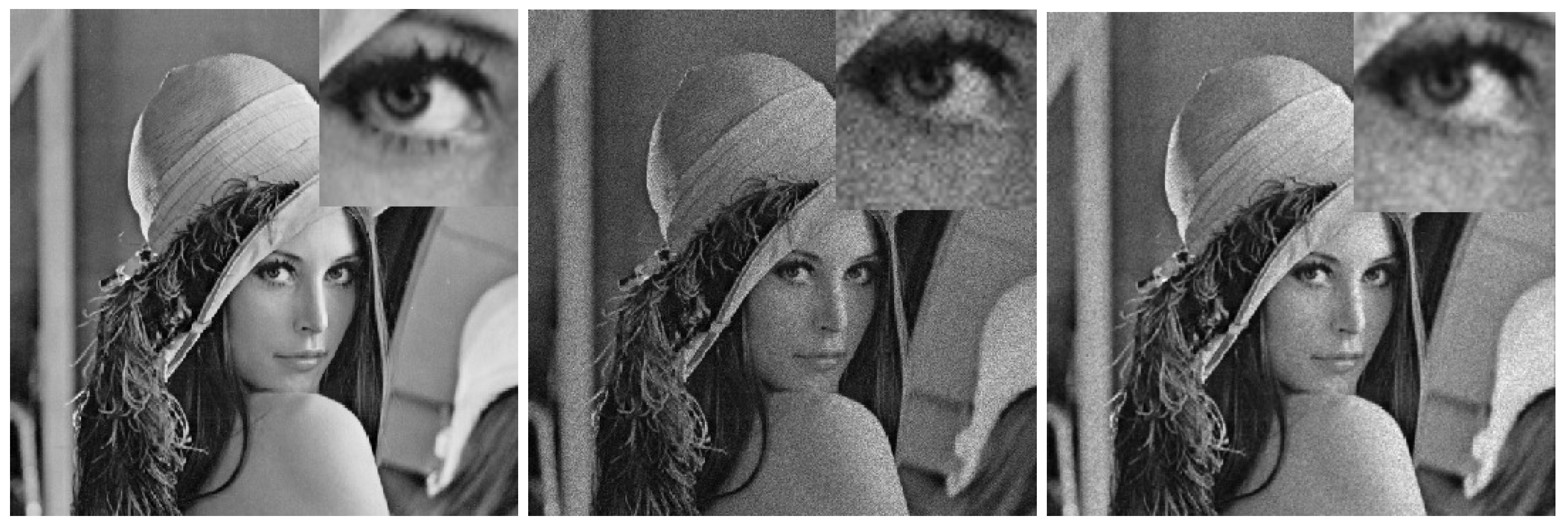
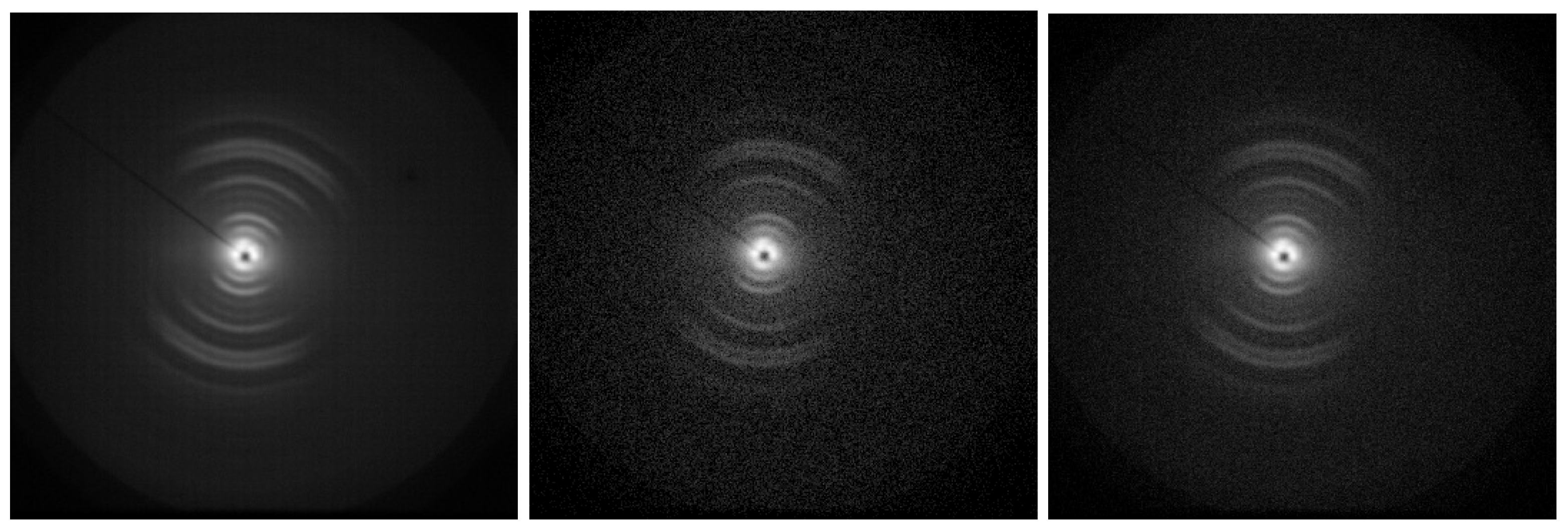
3. Results and Conclusions

The only parameters that are left in the numerical solution of Equation (2) are $\alpha$ and $\beta$ (the parameter $\lambda$, related to the non-dynamical field w, is proportional to the norm of the conjugate momentum density $|\nabla u|$ and it adiabatically changes [21]). While $\alpha =1.15$ is the highest value that can be used to guarantee stability without slowing down the convergence when the method is applied to an image affected by Gaussian noise (e.g., the classical Lenna image of Figure 1 and Figure 2), $\alpha =0.85$ appears to be the optimal solution for an application of the technique to the XRD two-dimensional patterns (e.g., Figure 3 and Figure 4). In fact, one has to balance between the need to use the highest possible value of ${\tilde{\omega }}^{-1}$ of Equation (2) to reduce the number of iterations to achieve the final reconstructed image and the stability requirement that fixes an upper bound for ${\tilde{\omega }}^{-1}$. The efficiency in image filtering is evaluated by measuring the peak signal-to-noise ratio (PSNR) defined as

$$\mathrm{PSNR}\stackrel{def.}{=}-20{log}_{10}\left({\displaystyle \frac{\sqrt{\langle |u-{\rho }_0{|}^2\rangle }}{max\left({\rho }_0\right)}}\right),$$

(3)

where ${\rho }_0$ is the original image without noise, u is the algorithm outcome (the restored image) and $\langle \dots \rangle$ denotes a sum over all the pixels of the images. This quantity is measured in decibels, and higher values correspond to better denoising. The parameter $\beta$ was varied in the method to obtain the highest possible values of PSNR.

Next to the Gaussian noise-affected images, the XRD experimental setups collect data on two-dimensional arrays, where a Poisson counting statistics accordingly needs noise reduction.

Wide-angle X-ray diffraction (WAXD) patterns are used to study the crystalline structure of materials, including fibers [6]. When fibers are analyzed using WAXD, the diffraction patterns provide information about the spacing and orientation of the crystalline regions within the fiber. In a typical WAXD pattern for fibers, one observes the following:

• Diffraction peaks, which indicate the presence of crystalline regions while their position and intensity can help determine the fiber’s crystallinity and the arrangement of its molecular chains.
• The intensity distribution of the peaks in the pattern, which can show how the crystalline regions are distributed and oriented relative to the fiber axis.
• Azimuthal scans, which can be used to study the orientation of the crystallites around the fiber axis, revealing information about fiber alignment and texture.

By analyzing these patterns, one gains insight into the structural properties of the fiber, such as its crystallinity, orientation, and potential mechanical properties.

To examine the effectiveness of the current approach on noisy data, I applied the model to denoise XRD patterns obtained from collagen molecules in tendon-derived collagens. Under various biochemical conditions, these molecules exhibit a super-organization into triple helices, displaying a preferred orientation as shown by the $\pi$-symmetric partial arcs in Figure 3, which replace the fully 2$\pi$-symmetric circles. This super-organization, along with a high-crystalline domain, contributes to the mechanical stiffness of the tissue (for details on sample preparation and experimental setup, the interested reader is referred to [5]). Figure 3 presents the XRD patterns, where the noisy image (center panel) was integrated over 2400 s, resulting in a maximum count below 1000, while the noiseless image (left panel) required 327,350 s, with maximum counts reaching around 60,000.

Small-angle and Wide-angle X-ray scattering (SAXS/WAXS) experiments were conducted at the X-ray Micro Imaging Laboratory (XMI-LAB [6]) on raw collagen flakes and processed collagen films. The setup included a Fr-E+SuperBright rotating copper anode microsource ($\lambda$ = 0.154 nm), a Confocal Max-Flux optics system, and a SAXS/WAXS three-pinhole camera. WAXS data were collected using a 250 × 160 mm² image plate detector (100 μm pixel size) with an off-line RAXIA reader. The samples were mounted on the holder, and data were gathered from three points on each sample. The spot size was ≈200 μm, with a detector distance of 10 cm, covering a scattering vector range of 3 to 35 nm⁻¹ (0.18–2.5 nm d-spacing).

The input image was processed for several values of the parameter $\beta$. The results for PSNR (initial and final values) for the optimal $\beta$ are illustrated in

Table 1. Improvement in the PSNR and SSIM values with the use of the denoising procedure in the cases of images with Gaussian (Lenna) and Poissonian (XRD) noise with the corresponding values of $\alpha$ and $\beta$.

Image	Lenna	Lenna	Rat Tendon	sam4
resolution	512 × 512	512 × 512	1024 × 1024	1600 × 2500
$\alpha$	1.15	1.15	0.85	0.85
$\beta$	2.0	2.0	1.25	1.25
noise	0.05	0.10	-	-
PSNR (ini.)	31.33	25.31	25.94	30.91
PSNR (fin.)	34.76	30.33	30.76	34.75
SSIM (ini.)	0.59	0.41	0.10	0.60
SSIM (fin.)	0.68	0.53	0.27	0.67

, while the algorithm outcome is shown in Figure 3 (right panel). The PSNR has trends similar to the case of Figure 1 and Figure 2 with Gaussian noise: it can be seen that the PSNR stays constant for the optimal $\beta$ value, after an initial stagger (essentially similar to the PSNR vs. time plot, as a function of $\beta$, illustrated in [7], although the LBM-inspired algorithm outperforms the one used in the reference). (See

Table 2. A comparison of the improvements in PSNR and SSIM values between the LBM (this work) and diffusion-driven ([7]) denoising methods, applied to images with Gaussian (Lenna) and Poisson (sam4) noise (* an extra digit is added to highlight the slight improvement).

Image	Lenna	Lenna	sam4
resolution	512 × 512	512 × 512	1600 × 2500
noise	0.05	0.10	-
PSNR (ini.)	31.33	25.31	30.91
PSNR (fin., LBM)	34.76	30.33	34.75
PSNR (fin., Diff.)	34.52	30.22	33.69
SSIM (ini.)	0.59	0.41	0.597 *
SSIM (fin., LBM)	0.68	0.53	0.67
SSIM (fin., Diff.)	0.64	0.46	0.601 *

for a comparison of the improvements in PSNR and SSIM values between the LBM and diffusion-driven [7] denoising methods.

Another example of WAXD fiber pattern denoising is the linen samples characterized in [22]: the samples consisted of threads approximately 1 cm in length and 0.2–0.6 mm in width. WAXS experiments were conducted on all linen samples at the X-ray Micro Imaging Laboratory (XMI-LAB). The laboratory equipment setup was similar to the one described above. The system also featured an X-ray scanning microscope. WAXS data were collected using an image plate (IP) detector with an offline Rigaku RAXIA-Di reader. Each linen sample, mounted directly on the sample holder, was measured for 1800 s. The spot size at the sample was approximately 200 μm, with the image plate detector positioned about 10 cm away. This setup provided access to scattering vector moduli (q = 4$\pi \times sin(\theta /\lambda )$) ranging from 1.5 to roughly 35 nm⁻¹. After calibration, the two-dimensional (2D) data were converted into one-dimensional (1D) profiles. For detailed information on the experimental setup and analysis, interested readers can refer to the original papers. The algorithm outcome is illustrated in Figure 4, where the close-up images on the upper-right corner show the improvement of the diffraction arc/ring details. The improvement of the corresponding Figure of Merit (PSNR) is reported in Table 1.

Thus, low-statistics two-dimensional images, sometimes affected by artifacts (e.g., experimental setup shadows), benefit from pre-processing denoising; the improvement of the PSNR can be appreciated in Table 1. In that respect, in order to stress the algorithmic efficiency, the values of another Figure of Merit are added, namely, the structure similarity (SSIM), as defined, for instance, in [23] and implemented in MatLab: PSNR/SSIM values increased for all cases analyzed in this paper; they are in agreement with the visual inspection of the images before/after applying the algorithm, as reported in Figure 1, Figure 2, Figure 3 and Figure 4.

In summary, while LBM-based image denoising is still an evolving field, it shows significant potential due to its ability to model complex noise processes and preserve the quality of important features in the images. Moreover, this study highlights its effectiveness in dealing with specific types of noise, such as Gaussian noise or Poissonian noise. Finally, advances in computational techniques and hardware have enhanced the efficiency of LBM-based X-ray diffraction image denoising: on the one hand, improved algorithms and parallel processing have made it feasible to apply these methods to high-resolution images and real-time processing scenario; on the other hand, its ability to model diffusion and transport processes leverages the inherent properties of the LBM to effectively remove noise on a well-established multi-scale and adaptive physics-grounded approach. Ongoing research and development are likely to further enhance its capabilities and broaden its applications. Studies have compared LBM-based denoising methods with traditional approaches such as Gaussian filtering, wavelet denoising, and non-local means: LBM methods often show improved performance in preserving edge details and structural information while effectively reducing noise. Furthermore, there is growing interest in combining LBM methods with machine learning techniques for image denoising: machine learning models are used to optimize LBM parameters or to refine denoising results, leading to improved performance and more adaptive solutions. Finally this versatile method could be efficiently embedded in a suite of integrated programs for X-ray imaging.

References

1. Pietsch, P.; Wood, V. X-Ray Tomography for Lithium Ion Battery Research: A Practical Guide. Annu. Rev. Mater. Res. 2017, 47, 451–479. [Google Scholar] [CrossRef]
2. Sibillano, T.; De Caro, L.; Scattarella, F.; Scarcelli, G.; Siliqi, D.; Altamura, D.; Liebi, M.; Ladisa, M.; Bunk, O.; Giannini, C. Interfibrillar packing of bovine cornea by table-top and synchrotron scanning SAXS microscopy. J. Appl. Crystallogr. 2016, 49, 1231–1239. [Google Scholar] [CrossRef] [PubMed]
3. Giannini, C.; Siliqi, D.; Bunk, O.; Beraudi, A.; Ladisa, M.; Altamura, D.; Stea, S.; Baruffaldi, F. Correlative Light and Scanning X-Ray Scattering Microscopy of Healthy and Pathologic Human Bone Sections. Sci. Rep. 2012, 2, 2045–2322. [Google Scholar] [CrossRef] [PubMed]
4. Giannini, C.; Siliqi, D.; Ladisa, M.; Altamura, D.; Diaz, A.; Beraudi, A.; Sibillano, T.; De Caro, L.; Stea, S.; Baruffaldic, F.; et al. Scanning SAXS–WAXS microscopy on osteoarthritis-affected bone—An age-related study. J. Appl. Crystallogr. 2014, 47, 110–117. [Google Scholar] [CrossRef]
5. Terzi, A.; Storelli, E.; Bettini, S.; Sibillano, T.; Altamura, D.; Salvatore, L.; Madaghiele, M.; Romano, A.; Siliqi, D.; Ladisa, M.; et al. Effects of processing on structural, mechanical and biological properties of collagen-based substrates for regenerative medicine. Sci. Rep. 2018, 8, 2045–2322. [Google Scholar] [CrossRef] [PubMed]
6. Altamura, D.; Lassandro, R.; Vittoria, F.A.; De Caro, L.; Ladisa, D.S.M.; Giannini, C. X-ray microimaging laboratory (XMI-LAB). J. Appl. Crystallogr. 2012, 45, 869–873. [Google Scholar] [CrossRef]
7. Ladisa, M.; Lamura, A. Diffusion-Driven X-Ray Two-Dimensional Patterns Denoising. Materials 2020, 13, 2773. [Google Scholar] [CrossRef] [PubMed]
8. Hendriksen, A.A.; Bührer, M.; Leone, L.; Merlini, M.; Vigano, N.; Pelt, D.M.; Marone, F.; di Michiel, M.; Batenburg, K.J. Deep denoising for multi-dimensional synchrotron X-ray tomography without high-quality reference data. Sci. Rep. 2021, 11, 2045–2322. [Google Scholar] [CrossRef] [PubMed]
9. Zhou, Z.; Li, C.; Bi, X.; Zhang, C.; Huang, Y.; Zhuang, J.; Hua, W.; Dong, Z.; Zhao, L.; Zhang, Y.; et al. A machine learning model for textured X-ray scattering and diffraction image denoising. npj Comput. Mater. 2023, 9, 2057–3960. [Google Scholar] [CrossRef]
10. Oppliger, J.; Denner, M.M.; Küspert, J.; Frison, R.; Wang, Q.; Morawietz, A.; Ivashko, O.; Dippel, A.C.; Zimmermann, M.v.; Biało, I.; et al. Weak signal extraction enabled by deep neural network denoising of diffraction data. Nat. Mach. Intell. 2024, 6, 180–186. [Google Scholar] [CrossRef] [PubMed]
11. Zhou, Z.; Li, C.; Fan, L.; Dong, Z.; Wang, W.; Liu, C.; Zhang, B.; Liu, X.; Zhang, K.; Wang, L.; et al. Denoising an X-ray image by exploring the power of its physical symmetry. J. Appl. Crystallogr. 2024, 57, 741–754. [Google Scholar] [CrossRef]
12. Landau, L.D.; Lifshitz, E.M. Fluid Mechanics, 2nd ed.; Pergamon Press: Oxford, England, 1987. [Google Scholar]
13. Chen, H.; Chen, S.; Matthaeus, W.H. Recovery of the Navier–Stokes equations using a lattice-gas Boltzmann method. Phys. Rev. A 1992, 45, R5339. [Google Scholar] [CrossRef] [PubMed]
14. He, X.; Luo, L.S. Lattice Boltzmann Model for the Incompressible Navier–Stokes Equation. J. Stat. Phys. 1997, 88, 927–944. [Google Scholar] [CrossRef]
15. He, X.; Luo, L.S. A priori derivation of the lattice Boltzmann equation. Phys. Rev. E 1997, 55, R6333. [Google Scholar] [CrossRef]
16. Landau, L.D.; Lifshitz, E.M. Statistical Physics (Part 1), 3rd ed.; Pergamon Press: Oxford, England, 1980. [Google Scholar]
17. Landau, L.D.; Lifshitz, E.M. Physical Kinetics, 1st ed.; Pergamon Press: Oxford, England, 1981. [Google Scholar]
18. Landau, L.D.; Lifshitz, E.M. Mechanics, 3rd ed.; Butterworth-Heinenann: Oxford, England, 1976. [Google Scholar]
19. Bhatnagar, P.; Gross, E.; Krook, M. A model for collision processes in gases. I. Small amplitude processes in charged and neutral one-component systems. Phys. Rev. 1954, 94, 511–525. [Google Scholar] [CrossRef]
20. Kaushal, S.; Ansumali, S.; Boghosian, B.; Johnson, M. The lattice Fokker–Planck equation for models of wealth distribution. Phil. Trans. R. Soc. A 2020, 378, 20190401. [Google Scholar] [CrossRef] [PubMed]
21. Canny, J. A Computational Approach to Edge Detection. IEEE Trans. Pattern Anal. Mach. Intell. 1986, PAMI-8, 679–698. [Google Scholar] [CrossRef]
22. De Caro, L.; Giannini, C.; Lassandro, R.; Scattarella, F.; Sibillano, T.; Matricciani, E.; Fanti, G. X-Ray Dating of Ancient Linen Fabrics. Heritage 2019, 2, 2763–2783. [Google Scholar] [CrossRef]
23. Wang, Z.; Bovik, A.C.; Sheikh, H.R.; Simoncelli, E.P. Image Quality Assessment: From Error Visibility to Structural Similarity. IEEE Trans. Image Process. 2004, 13, 600–612. [Google Scholar] [CrossRef] [PubMed]
Figure 1. Noiseless image (left): original Lenna image with clear details and no visible distortion. Noisy image (centre): the same image affected by Gaussian noise 5 % , compromising detail and clarity. Denoised outcome (right): improved image after applying the denoising algorithm. The close-up images on the upper-right corner reveal restored details and reduced noise.
Crystals 15 00051 g001
Figure 2. Noiseless image (left): original Lenna image with clear details and no visible distortion. Noisy image (centre): the same image affected by Gaussian noise 10 % , compromising detail and clarity. Denoised outcome (right): improved image after applying the denoising algorithm. The close-up images on the upper-right corner reveal restored details and reduced noise.
Crystals 15 00051 g002
Figure 3. Noiseless image (left): high statistics rat tendon image with clear details and a preferred orientation displayed by the π -symmetric partial arcs. Noisy image (centre): the same image affected by Poissonian noise due to a collection time of 2400 s only. Denoised outcome (right): improved image after applying the denoising algorithm.
Crystals 15 00051 g003
Figure 4. Noiseless image (left): original high-count-rate sam4 XRD image with clear details. Noisy image (centre): the same image affected by Poissonian noise due to a low count statistics. Denoised outcome (right): improved image after applying the denoising algorithm. The close-up images on the upper-right corner spot the reduced noise.
Crystals 15 00051 g004