
Quantum Chemical Topological Analysis of [2Fe2S] Core in Novel [FeFe]-Hydrogenase Mimics


Abstract

1. Introduction
2. Computational Details
3. Results and Discussion
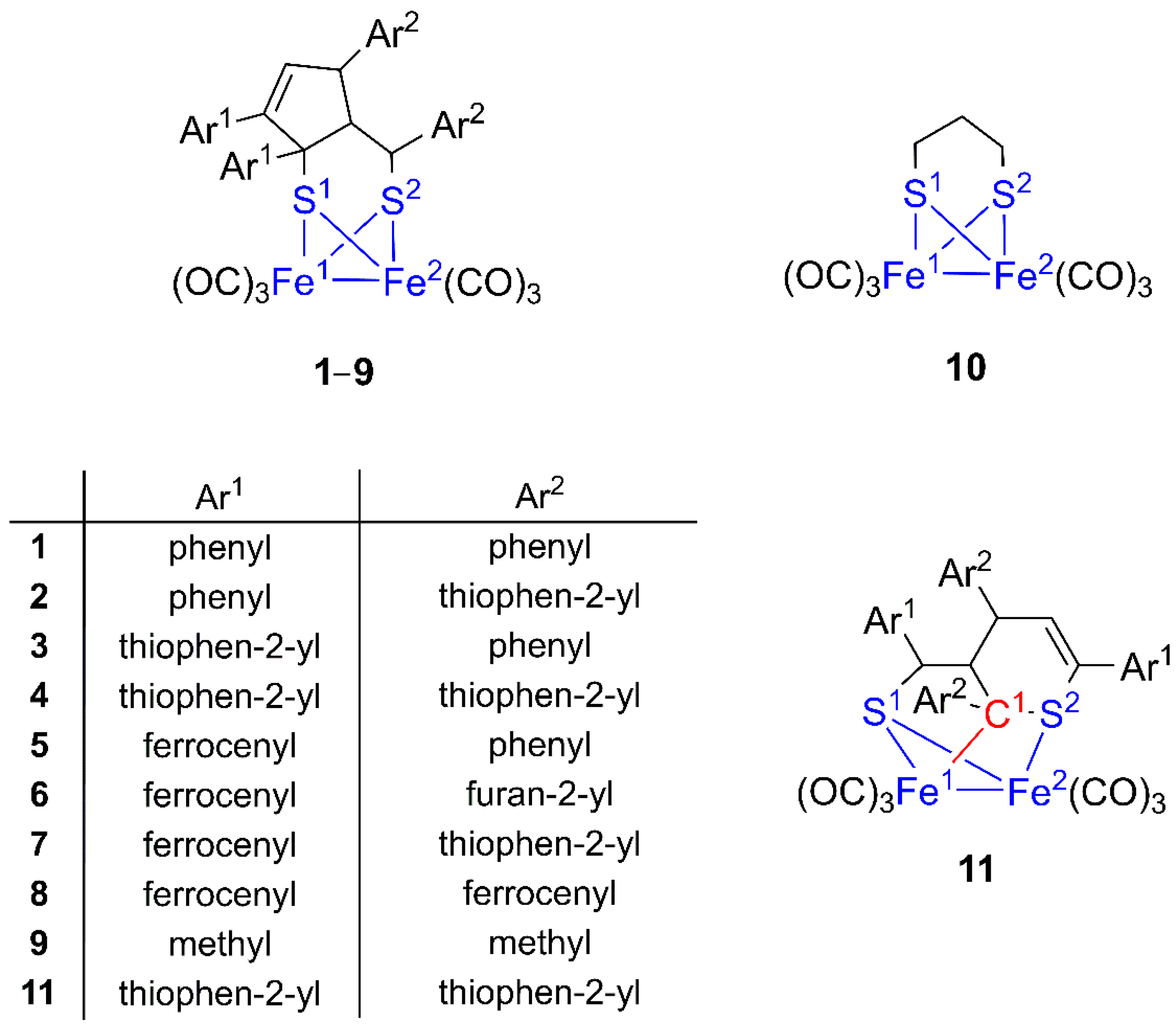
3.1. Molecular Geometries
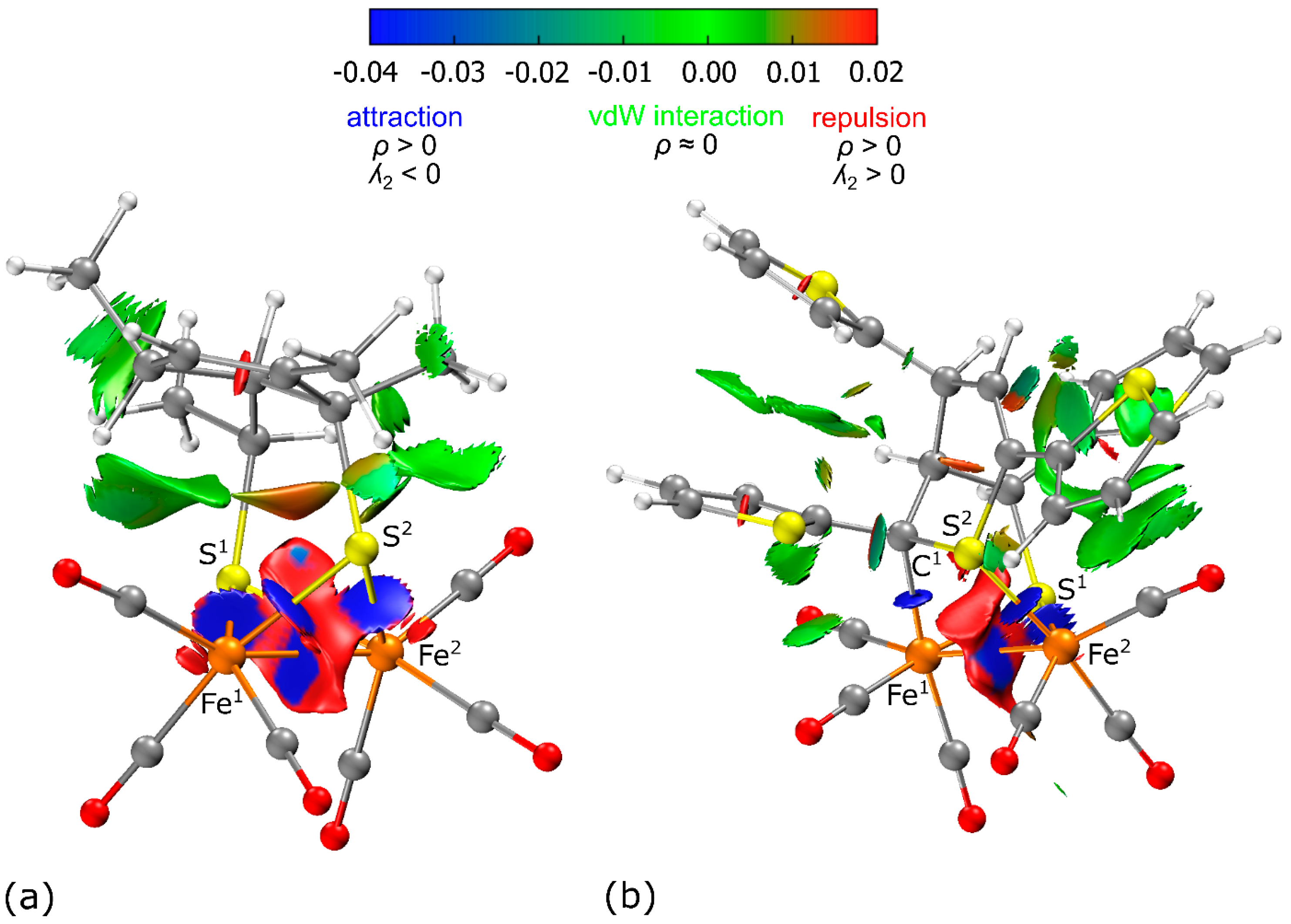
3.2. IRI Analysis
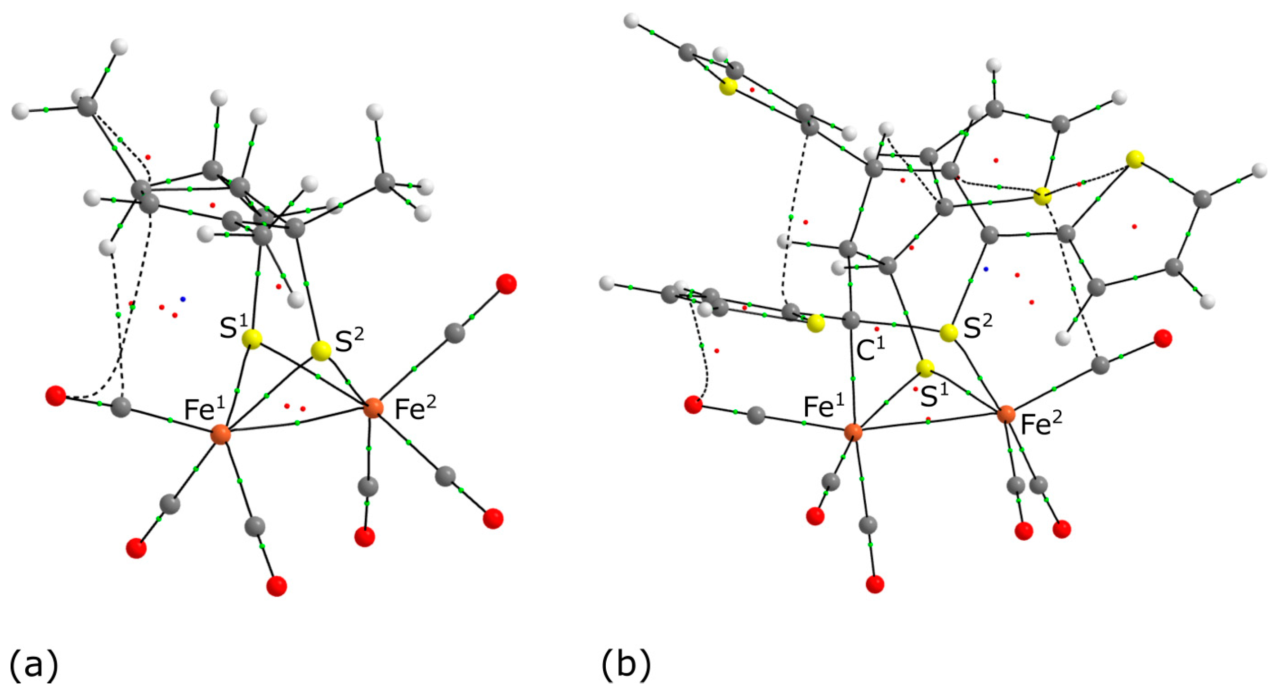
3.3. QTAIM Analysis
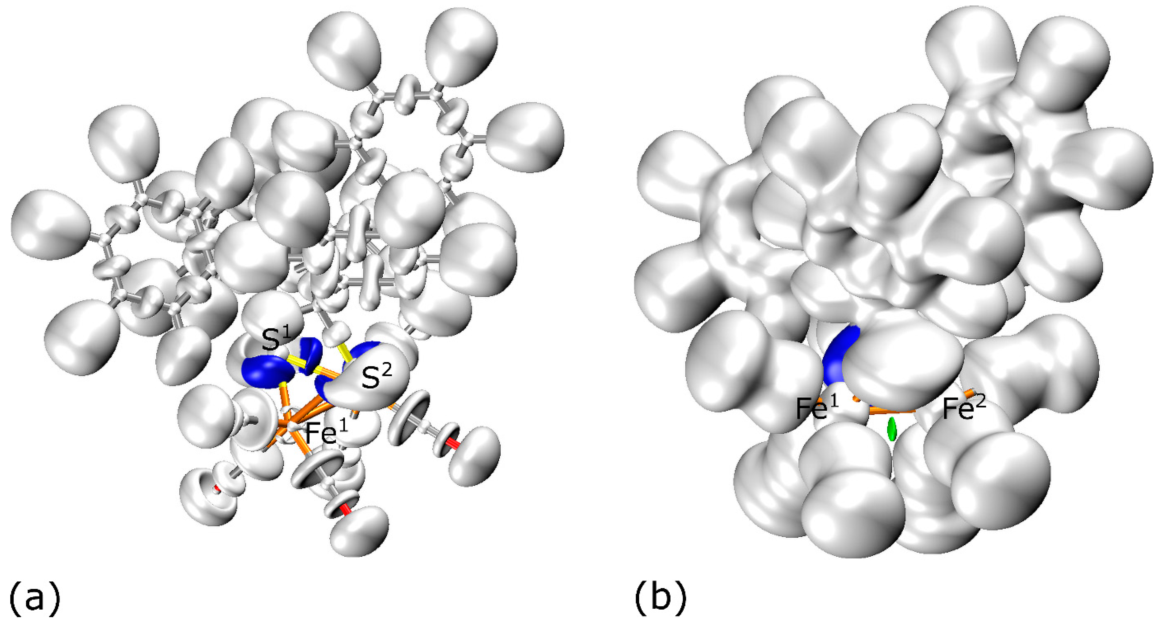
3.4. SF Analysis
3.5. ELF Analysis
3.6. IQA and IQF Analyses
4. Conclusions
Supplementary Materials
Funding
Data Availability Statement
Acknowledgments
Conflicts of Interest
References
- Evans, D.J.; Pickett, C.J. Chemistry and the Hydrogenases. Chem. Soc. Rev. 2003, 32, 268–275. [Google Scholar] [CrossRef] [PubMed]
- Liu, X.; Ibrahim, S.K.; Tard, C.; Pickett, C.J. Iron-Only Hydrogenase: Synthetic, Structural and Reactivity Studies of Model Compounds. Coord. Chem. Rev. 2005, 249, 1641–1652. [Google Scholar] [CrossRef]
- Vignais, P.M.; Billoud, B. Occurrence, Classification, and Biological Function of Hydrogenases: An Overview. Chem. Rev. 2007, 107, 4206–4272. [Google Scholar] [CrossRef]
- Schilter, D.; Camara, J.M.; Huynh, M.T.; Hammes-Schiffer, S.; Rauchfuss, T.B. Hydrogenase Enzymes and Their Synthetic Models: The Role of Metal Hydrides. Chem. Rev. 2016, 116, 8693–8749. [Google Scholar] [CrossRef] [PubMed]
- Wittkamp, F.; Senger, M.; Stripp, S.T.; Apfel, U.-P. [FeFe]-Hydrogenases: Recent Developments and Future Perspectives. Chem. Commun. 2018, 54, 5934–5942. [Google Scholar] [CrossRef]
- Gao, S.; Liu, Y.; Shao, Y.; Jiang, D.; Duan, Q. Iron Carbonyl Compounds with Aromatic Dithiolate Bridges as Organometallic Mimics of [FeFe] Hydrogenases. Coord. Chem. Rev. 2020, 402, 213081. [Google Scholar] [CrossRef]
- Hogarth, G. An Unexpected Leading Role for [Fe2(CO)6(μ-Pdt)] in Our Understanding of [FeFe]-H2ases and the Search for Clean Hydrogen Production. Coord. Chem. Rev. 2023, 490, 215174. [Google Scholar] [CrossRef]
- Ji, H.; Wan, L.; Gao, Y.; Du, P.; Li, W.; Luo, H.; Ning, J.; Zhao, Y.; Wang, H.; Zhang, L.; et al. Hydrogenase as the Basis for Green Hydrogen Production and Utilization. J. Energy Chem. 2023, 85, 348–362. [Google Scholar] [CrossRef]
- Grinberg, I.; Ben-Zvi, O.; Adler-Abramovich, L.; Yacoby, I. Peptide Self-assembly as a Strategy for Facile Immobilization of Redox Enzymes on Carbon Electrodes. Carbon Energy 2023, 5, e411. [Google Scholar] [CrossRef]
- Mulder, D.W.; Guo, Y.; Ratzloff, M.W.; King, P.W. Identification of a Catalytic Iron-Hydride at the H-cluster of [FeFe]-Hydrogenase. J. Am. Chem. Soc. 2017, 139, 83–86. [Google Scholar] [CrossRef]
- Li, Y.; Rauchfuss, T.B. Synthesis of Diiron(I) Dithiolato Carbonyl Complexes. Chem. Rev. 2016, 116, 7043–7077. [Google Scholar] [CrossRef] [PubMed]
- Buday, P.; Seeber, P.; Zens, C.; Abul-Futouh, H.; Görls, H.; Gräfe, S.; Matczak, P.; Kupfer, S.; Weigand, W.; Mlostoń, G. Iron(0)-Mediated Stereoselective (3+2)-Cycloaddition of Thiochalcones via a Diradical Intermediate. Chem. Eur. J. 2020, 26, 11412–11416. [Google Scholar] [CrossRef] [PubMed]
- Lansing, J.C.; Camara, J.M.; Gray, D.E.; Rauchfuss, T.B. Hydrogen Production Catalyzed by Bidirectional, Biomimetic Models of the [FeFe]-Hydrogenase Active Site. Organometallics 2014, 33, 5897–5906. [Google Scholar] [CrossRef]
- Kositzki, R.; Mebs, S.; Schuth, N.; Leidel, N.; Schwartz, L.; Karnahl, M.; Wittkamp, F.; Daunke, D.; Grohmann, A.; Apfel, U.-P.; et al. Electronic and Molecular Structure Relations in Diiron Compounds Mimicking the [FeFe]-Hydrogenase Active Site Studied by X-Ray Spectroscopy and Quantum Chemistry. Dalton Trans. 2017, 46, 12544–12557. [Google Scholar] [CrossRef]
- Matczak, P.; Domagała, M.; Domagała, S. Conformers of Diheteroaryl Ketones and Thioketones: A Quantum Chemical Study of Their Properties and Fundamental Intramolecular Energetic Effects. Struct. Chem. 2016, 27, 855–869. [Google Scholar] [CrossRef]
- Gröber, S.; Matczak, P.; Domagała, S.; Weisheit, T.; Görls, H.; Düver, A.; Mlostoń, G.; Weigand, W. Diferrocenyl Thioketone: Reactions with (Bisphosphane)Pt(0) Complexes—Electrochemical and Computational Studies. Materials 2019, 12, 2832. [Google Scholar] [CrossRef] [PubMed]
- Matczak, P.; Kupfer, S.; Mlostoń, G.; Buday, P.; Görls, H.; Weigand, W. Metal–Ligand Bonding in Tricarbonyliron(0) Complexes Bearing Thiochalcone Ligands. New J. Chem. 2022, 46, 12924–12933. [Google Scholar] [CrossRef]
- Matczak, P.; Domagała, S.; Weigand, W.; Mlostoń, G. A Comparative Analysis of UV–Vis Transitions in Hetaryl and Ferrocenyl Thioketones. Chem. Phys. 2023, 570, 111901. [Google Scholar] [CrossRef]
- Matczak, P.; Buday, P.; Kupfer, S.; Görls, H.; Mlostoń, G.; Weigand, W. Probing the Performance of DFT in the Structural Characterization of [FeFe] Hydrogenase Models. J. Comput. Chem. 2025, 46, e27515. [Google Scholar] [CrossRef]
- Popelier, P.L.A. On Quantum Chemical Topology. In Applications of Topological Methods in Molecular Chemistry; Chauvin, R., Lepetit, C., Silvi, B., Alikhani, E., Eds.; Challenges and Advances in Computational Chemistry and Physics; Springer International Publishing: Cham, Switzerland, 2016. [Google Scholar]
- Bader, R.F.W. Atoms in Molecules: A Quantum Theory; Clarendon: Oxford, UK, 1990. [Google Scholar]
- Silvi, B.; Savin, A. Classification of Chemical Bonds Based on Topological Analysis of Electron Localization Functions. Nature 1994, 371, 683–686. [Google Scholar] [CrossRef]
- Johnson, E.R.; Keinan, S.; Mori-Sánchez, P.; Contreras-García, J.; Cohen, A.J.; Yang, W. Revealing Noncovalent Interactions. J. Am. Chem. Soc. 2010, 132, 6498–6506. [Google Scholar] [CrossRef] [PubMed]
- Contreras-García, J.; Johnson, E.R.; Keinan, S.; Chaudret, R.; Piquemal, J.-P.; Beratan, D.N.; Yang, W. NCIPLOT: A Program for Plotting Noncovalent Interaction Regions. J. Chem. Theory Comput. 2011, 7, 625–632. [Google Scholar] [CrossRef]
- Lu, T.; Chen, Q. Interaction Region Indicator: A Simple Real Space Function Clearly Revealing Both Chemical Bonds and Weak Interactions. Chem. Methods 2021, 1, 231–239. [Google Scholar] [CrossRef]
- Blanco, M.A.; Martín Pendás, A.; Francisco, E. Interacting Quantum Atoms: A Correlated Energy Decomposition Scheme Based on the Quantum Theory of Atoms in Molecules. J. Chem. Theory Comput. 2005, 1, 1096–1109. [Google Scholar] [CrossRef] [PubMed]
- Guevara-Vela, J.M.; Francisco, E.; Rocha-Rinza, T.; Pendás, Á.M. Interacting Quantum Atoms—A Review. Molecules 2020, 25, 4028. [Google Scholar] [CrossRef] [PubMed]
- Macchi, P.; Sironi, A. Chemical Bonding in Transition Metal Carbonyl Clusters: Complementary Analysis of Theoretical and Experimental Electron Densities. Coord. Chem. Rev. 2003, 238–239, 383–412. [Google Scholar] [CrossRef]
- Frenking, G.; Fernández, I.; Holzmann, N.; Pan, S.; Krossing, I.; Zhou, M. Metal−CO Bonding in Mononuclear Transition Metal Carbonyl Complexes. JACS Au 2021, 1, 623–645. [Google Scholar] [CrossRef]
- Bertini, L.; Greco, C.; De Gioia, L.; Fantucci, P. DFT/TDDFT Exploration of the Potential Energy Surfaces of the Ground State and Excited States of Fe2(S2C3H6)(CO)6: A Simple Functional Model of the [FeFe] Hydrogenase Active Site. J. Phys. Chem. A 2009, 113, 5657–5670. [Google Scholar] [CrossRef]
- Bertini, L.; Greco, C.; Bruschi, M.; Fantucci, P.; De Gioia, L. CO Affinity and Bonding Properties of [FeFe] Hydrogenase Active Site Models. A DFT Study. Organometallics 2010, 29, 2013–2025. [Google Scholar] [CrossRef]
- Giles, L.J.; Grigoropoulos, A.; Szilagyi, R.K. Electron and Spin Density Topology of the H-Cluster and Its Biomimetic Complexes. Eur. J. Inorg. Chem. 2011, 2011, 2677–2690. [Google Scholar] [CrossRef]
- Arrigoni, F.; Zampella, G.; De Gioia, L.; Greco, C.; Bertini, L. The Photochemistry of Fe2(S2C3H6)(CO)6(µ-CO) and Its Oxidized Form, Two Simple [FeFe]-Hydrogenase CO-Inhibited Models. A DFT and TDDFT Investigation. Inorganics 2021, 9, 16. [Google Scholar] [CrossRef]
- Lyon, E.J.; Georgakaki, I.P.; Reibenspies, J.H.; Darensbourg, M.Y. Carbon Monoxide and Cyanide Ligands in a Classical Organometallic Complex Model for Fe-Only Hydrogenase. Angew. Chem. Int. Ed. 1999, 38, 3178–3180. [Google Scholar] [CrossRef]
- Staroverov, V.N.; Scuseria, G.E.; Tao, J.; Perdew, J.P. Comparative Assessment of a New Nonempirical Density Functional: Molecules and Hydrogen-Bonded Complexes. J. Chem. Phys. 2003, 119, 12129–12137. [Google Scholar] [CrossRef]
- Weigend, F.; Ahlrichs, R. Balanced Basis Sets of Split Valence, Triple Zeta Valence and Quadruple Zeta Valence Quality for H to Rn: Design and Assessment of Accuracy. Phys. Chem. Chem. Phys. 2005, 7, 3297–3305. [Google Scholar] [CrossRef]
- Becke, A.D. Density-Functional Thermochemistry. III. The Role of Exact Exchange. J. Chem. Phys. 1993, 98, 5648–5652. [Google Scholar] [CrossRef]
- Hertwig, R.H.; Koch, W. On the Parameterization of the Local Correlation Functional. What Is Becke-3-LYP? Chem. Phys. Lett. 1997, 268, 345–351. [Google Scholar] [CrossRef]
- Gatti, C.; Cargnoni, F.; Bertini, L. Chemical Information from the Source Function. J. Comput. Chem. 2003, 24, 422–436. [Google Scholar] [CrossRef] [PubMed]
- Martín Pendás, A.; Blanco, M.A.; Francisco, E. The Nature of the Hydrogen Bond: A Synthesis from the Interacting Quantum Atoms Picture. J. Chem. Phys. 2006, 125, 184112. [Google Scholar] [CrossRef] [PubMed]
- Ahlrichs, R.; Armbruster, M.K.; Bachorz, R.A.; Bahmann, H.; Baldes, A.; Bär, M.; Baron, H.; Bauernschmitt, R.; Bischof, F.A.; Böcker, S.; et al. TURBOMOLE 7.7; A Development of University of Karlsruhe and Forschungszentrum Karlsruhe GmbH, 1989–2007; TURBOMOLE GmbH: Karlsruhe, Germany, 2022. [Google Scholar]
- Frisch, M.J.; Trucks, G.W.; Schlegel, H.B.; Scuseria, G.E.; Robb, M.A.; Cheeseman, J.R.; Scalmani, G.; Barone, V.; Petersson, G.A.; Nakatsuji, H.; et al. Gaussian 16, Rev. C.01; Gaussian, Inc.: Wallingford, CT, USA, 2016. [Google Scholar]
- Lu, T.; Chen, F. Multiwfn: A Multifunctional Wavefunction Analyzer. J. Comput. Chem. 2012, 33, 580–592. [Google Scholar] [CrossRef]
- Keith, T.A. AIMAll 19.10.12; TK Gristmill Software: Overland Park, KS, USA, 2019. [Google Scholar]
- Humphrey, W.; Dalke, A.; Schulten, K. VMD—Visual Molecular Dynamics. J. Mol. Graph. 1996, 14, 33–38. [Google Scholar] [CrossRef] [PubMed]
- Zhao, C.; Wu, R.; Zhang, S.; Hong, X. Benchmark Study of Density Functional Theory Methods in Geometry Optimization of Transition Metal−Dinitrogen Complexes. J. Phys. Chem. A 2023, 127, 6791–6803. [Google Scholar] [CrossRef] [PubMed]
- Hargittai, M.; Hargittai, I. Gas-Solid Molecular Structure Differences. Phys. Chem. Minerals 1987, 14, 413–425. [Google Scholar] [CrossRef]
- Pyykkö, P.; Atsumi, M. Molecular Single-Bond Covalent Radii for Elements 1–118. Chem. Eur. J. 2009, 15, 186–197. [Google Scholar] [CrossRef] [PubMed]
- Bader, R.F.W. A Bond Path: A Universal Indicator of Bonded Interactions. J. Phys. Chem. A 1998, 102, 7314–7323. [Google Scholar] [CrossRef]
- Farrugia, L.J.; Macchi, P. Bond Orders in Metal–Metal Interactions through Electron Density Analysis. Struct. Bond. 2012, 146, 127–158. [Google Scholar]
- Malcek, M.; Vénosová, B.; Puškárová, I.; Kožíšek, J.; Gall, M.; Bucinský, L. Coordination Bonding in Dicopper and Dichromium Tetrakis (μ-Acetato)-Diaqua Complexes: Nature, Strength, Length, and Topology. J. Comput. Chem. 2020, 41, 698–714. [Google Scholar] [CrossRef] [PubMed]
- Farrugia, L.J.; Evans, C.; Senn, H.M.; Hänninen, M.M.; Sillanpäa, R. QTAIM View of Metal−Metal Bonding in Di- and Trinuclear Disulfido Carbonyl Clusters. Organometallics 2012, 31, 2559–2570. [Google Scholar] [CrossRef]
- Cremer, D.; Kraka, E. A Description of the Chemical Bond in Terms of Local Properties of Electron Density and Energy. Croat. Chem. Acta 1984, 57, 1259–1281. [Google Scholar]
- Bianchi, R.; Gervasio, G.; Marabello, D. Experimental Electron Density Analysis of Mn2(CO)10: Metal-Metal and Metal-Ligand Bond Characterization. Inorg. Chem. 2000, 39, 2360–2366. [Google Scholar] [CrossRef] [PubMed]
- Macchi, P.; Proserpio, D.M.; Sironi, A. Experimental Electron Density in a Transition Metal Dimer: Metal-Metal and Metal-Ligand Bonds. J. Am. Chem. Soc. 1998, 120, 13429–13435. [Google Scholar] [CrossRef]
- Fradera, X.; Austen, M.A.; Bader, R.F.W. The Lewis Model and Beyond. J. Phys. Chem. A 1999, 103, 304–314. [Google Scholar] [CrossRef]
- Rose, K.; Shadle, S.E.; Glaser, T.; de Vries, S.; Cherepanov, A.; Canters, G.W.; Hedman, B.; Hodgson, K.O.; Solomon, E.I. Investigation of the Electronic Structure of 2Fe-2S Model Complexes and the Rieske Protein Using Ligand K-Edge X-Ray Absorption Spectroscopy. J. Am. Chem. Soc. 1999, 121, 2353–2363. [Google Scholar] [CrossRef]
- Harris, T.V.; Szilagyi, R.K. Iron–Sulfur Bond Covalency from Electronic Structure Calculations for Classical Iron–Sulfur Clusters. J. Comput. Chem. 2014, 35, 540–552. [Google Scholar] [CrossRef] [PubMed]
- Lee, C.-R.; Hsu, I.-J.; Chen, H.-T.; Lee, G.-H.; Wang, Y. Charge Density Studies on [(NO)Fe(S2C6H4)2][PPN] and [(NO)3Fe(S2C6H4)3] Complexes. C. R. Chim. 2012, 15, 237–249. [Google Scholar] [CrossRef]
- Lebon, A.; Orain, P.-Y.; Memboeuf, A. Understanding the CO Dissociation in [Fe(CN)2(CO)2(Dithiolate)]2− Complexes with Quantum Chemical Topology Tools. J. Phys. Chem. A 2017, 121, 7031–7041. [Google Scholar] [CrossRef]
- Espinosa, E.; Alkorta, I.; Elguero, J.; Molins, E. From Weak to Strong Interactions: A Comprehensive Analysis of the Topological and Energetic Properties of the Electron Density Distribution Involving X–H···F–Y Systems. J. Chem. Phys. 2002, 117, 5529–5542. [Google Scholar] [CrossRef]
- Reinhold, J.; Kluge, O.; Mealli, C. Integration of Electron Density and Molecular Orbital Techniques to Reveal Questionable Bonds: The Test Case of the Direct Fe−Fe Bond in Fe2(CO)9. Inorg. Chem. 2007, 46, 7142–7147. [Google Scholar] [CrossRef] [PubMed]
- Gatti, C.; Lasi, D. Source Function Description of Metal–Metal Bonding in d-Block Organometallic Compounds. Faraday Discuss. 2007, 135, 55–78. [Google Scholar] [CrossRef]
- Berski, S.; Gutsev, G.L.; Mochena, M.D.; Andres, J. Toward Understanding the Electron Density Distribution in Magnetic Clusters: Insight from the ELF and AIM Analyses of Ground-State Fe4. J. Phys. Chem. A 2004, 108, 6025–6031. [Google Scholar] [CrossRef]
- Viciano, I.; Berski, S.; Marti, S.; Andres, J. New Insight into the Electronic Structure of Iron(IV)-Oxo Porphyrin Compound I. A Quantum Chemical Topological Analysis. J. Comput. Chem. 2013, 34, 780–789. [Google Scholar] [CrossRef] [PubMed]
- Tiana, D.; Francisco, E.; Macchi, P.; Sironi, A.; Pendás, A.M. An Interacting Quantum Atoms Analysis of the Metal−Metal Bond in [M2(CO)8]n Systems. J. Phys. Chem. A 2015, 119, 2153–2160. [Google Scholar] [CrossRef] [PubMed]
- Martín Pendás, A.; Francisco, E.; Blanco, M.A.; Gatti, C. Bond Paths as Privileged Exchange Channels. Chem. Eur. J. 2007, 13, 9362–9371. [Google Scholar] [CrossRef]
- Schwab, D.E.; Tard, C.; Brecht, E.; Peters, J.W.; Pickett, C.J.; Szilagyi, R.K. On the Electronic Structure of the Hydrogenase H-Cluster. Chem. Commun. 2006, 3696–3698. [Google Scholar] [CrossRef]
- Chang, C.H. Computational Chemical Analysis of [FeFe] Hydrogenase H-Cluster Analogues to Discern Catalytically Relevant Features of the Natural Diatomic Ligand Configuration. J. Phys. Chem. A 2011, 115, 8691–8704. [Google Scholar] [CrossRef] [PubMed]
- Benediktsson, B.; Bjornsson, R. Analysis of the Geometric and Electronic Structure of Spin-Coupled Iron−sulfur Dimers with Broken-Symmetry DFT: Implications for FeMoco. J. Chem. Theory Comput. 2022, 18, 1437–1457. [Google Scholar] [CrossRef]
- Eichkorn, K.; Treutler, O.; Öhm, H.; Häser, M.; Ahlrichs, R. Auxiliary Basis Sets to Approximate Coulomb Potentials. Chem. Phys. Lett. 1995, 240, 283–290. [Google Scholar] [CrossRef]
- Eichkorn, K.; Weigend, F.; Treutler, O.; Ahlrichs, R. Auxiliary Basis Sets for Main Row Atoms and Transition Metals and Their Use to Approximate Coulomb Potentials. Theor. Chem. Acc. 1997, 97, 119–124. [Google Scholar] [CrossRef]
- Weigend, F. Accurate Coulomb-Fitting Basis Sets for H to Rn. Phys. Chem. Chem. Phys. 2006, 8, 1057–1065. [Google Scholar] [CrossRef] [PubMed]
- Furness, J.W.; Kaplan, A.D.; Ning, J.; Perdew, J.P.; Sun, J. Accurate and Numerically Efficient r2SCAN Meta-Generalized Gradient Approximation. J. Phys. Chem. Lett. 2020, 11, 8208–8215. [Google Scholar] [CrossRef]
- Kleinhaus, J.T.; Wittkamp, F.; Yadav, S.; Siegmund, D.; Apfel, U.-P. [FeFe]-Hydrogenases: Maturation and Reactivity of Enzymatic Systems and Overview of Biomimetic Models. Chem. Soc. Rev. 2021, 50, 1668–1784. [Google Scholar] [CrossRef] [PubMed]

| Complex | Fe1–Fe2 | Fe1–S1 | Fe1–S2 | Fe2–S1 | Fe2–S2 | Average Fe–S |
|---|---|---|---|---|---|---|
| 1 | 247.3 (249.9) | 227.9 (230.4) | 231.2 (234.0) | 231.0 (233.7) | 228.4 (230.6) | 229.6 (232.2) |
| 2 | 247.6 (249.9) | 227.7 (230.3) | 230.7 (233.9) | 230.6 (233.5) | 228.1 (230.7) | 229.3 (232.1) |
| 3 | 247.6 (250.2) [251.5] | 227.5 (230.1) [224.1] | 230.7 (233.5) [227.9] | 229.8 (232.6) [226.2] | 228.4 (230.7) [225.1] | 229.1 (231.7) |
| 4 | 247.8 (250.0) | 227.5 (230.2) | 230.5 (233.8) | 229.5 (232.9) | 228.3 (230.8) | 229.0 (231.9) |
| 5 | 248.9 (251.3) [250.8] | 227.0 (229.3) [224.1] | 229.2 (232.1) [227.3] | 227.4 (230.1) [225.3] | 228.2 (230.6) [224.9] | 228.0 (230.5) |
| 6 | 248.5 (251.0) | 228.2 (230.8) | 228.4 (230.8) | 227.2 (229.5) | 229.5 (232.4) | 228.3 (230.9) |
| 7 | 248.7 (251.3) [251.5] | 227.9 (230.3) [223.2] | 228.3 (230.7) [224.8] | 226.9 (229.2) [225.2] | 229.6 (232.2) [225.0] | 228.2 (230.6) |
| 8 | 248.6 (251.1) | 228.0 (230.5) | 228.2 (230.8) | 226.7 (229.2) | 229.7 (232.3) | 228.2 (230.7) |
| 9 | 248.2 (250.8) | 227.2 (229.7) | 229.8 (232.4) | 228.3 (230.9) | 228.6 (230.9) | 228.5 (231.0) |
| 10 | 248.4 (250.9) [251.0] | 228.2 (230.8) [224.9] | 228.2 (230.8) [225.4] | 228.9 (231.7) [224.9] | 228.9 (231.7) [225.4] | 228.6 (231.3) |
| 11 | 260.3 (264.3) [263.7] | 223.8 (225.5) [221.4] | 286.7 (291.5) [286.5] | 227.5 (230.4) [224.3] | 229.7 (233.1) [226.4] | 241.9 (245.1) |
| Complex | ρBCP | ∇2ρBCP | |VBCP|/GBCP | GBCP/ρBCP | HBCP | δ |
|---|---|---|---|---|---|---|
| 1 | 0.0527 (0.0528) | 0.0444 (0.0686) | 1.604 (1.443) | 0.5312 (0.5833) | −0.0169 (−0.0136) | 0.470 (0.477) |
| 2 | 0.0526 (0.0527) | 0.0439 (0.0685) | 1.606 (1.442) | 0.5297 (0.5826) | −0.0169 (−0.0136) | 0.470 (0.477) |
| 3 | 0.0525 (0.0526) | 0.0442 (0.0691) | 1.604 (1.439) | 0.5313 (0.5849) | −0.0169 (−0.0135) | 0.471 (0.477) |
| 4 | 0.0524 (0.0525) | 0.0440 (0.0693) | 1.606 (1.437) | 0.5313 (0.5858) | −0.0169 (−0.0134) | 0.470 (0.476) |
| 5 | 0.0517 (0.0518) | 0.0430 (0.0694) | 1.608 (1.429) | 0.5298 (0.5862) | −0.0167 (−0.0130) | 0.467 (0.474) |
| 6 | 0.0519 (0.0520) | 0.0432 (0.0689) | 1.607 (1.434) | 0.5295 (0.5842) | −0.0167 (−0.0132) | 0.471 (0.478) |
| 7 | 0.0518 (0.0520) | 0.0429 (0.0689) | 1.608 (1.433) | 0.5289 (0.5841) | −0.0167 (−0.0131) | 0.470 (0.477) |
| 8 | 0.0518 (0.0520) | 0.0435 (0.0695) | 1.605 (1.430) | 0.5311 (0.5868) | −0.0167 (−0.0131) | 0.467 (0.474) |
| 9 | 0.0521 (0.0521) | 0.0441 (0.0700) | 1.603 (1.429) | 0.5331 (0.5888) | −0.0168 (−0.0132) | 0.469 (0.475) |
| 10 | 0.0518 (0.0517) | 0.0451 (0.0717) | 1.596 (1.418) | 0.5383 (0.5954) | −0.0166 (−0.0129) | 0.479 (0.484) |
| 11 | 0.0445 (n/a) | 0.0270 (n/a) | 1.683 (n/a) | 0.4777 (n/a) | −0.0145 (n/a) | 0.429 (0.433) |
| Complex | ρBCP | ∇2ρBCP | |VBCP|/GBCP | GBCP/ρBCP | HBCP | δ |
|---|---|---|---|---|---|---|
| 1 | 0.0744 (0.0790) | 0.2306 (0.1749) | 1.159 (1.369) | 0.9213 (0.8766) | −0.0109 (−0.0255) | 0.688 (0.721) |
| 2 | 0.0747 (0.0793) | 0.2313 (0.1753) | 1.160 (1.370) | 0.9218 (0.8768) | −0.0110 (−0.0257) | 0.688 (0.722) |
| 3 | 0.0749 (0.0796) | 0.2336 (0.1772) | 1.159 (1.368) | 0.9272 (0.8814) | −0.0111 (−0.0258) | 0.689 (0.723) |
| 4 | 0.0749 (0.0796) | 0.2338 (0.1774) | 1.159 (1.368) | 0.9279 (0.8821) | −0.0110 (−0.0258) | 0.687 (0.721) |
| 5 | 0.0765 (0.0811) | 0.2296 (0.1719) | 1.174 (1.385) | 0.9081 (0.8620) | −0.0121 (−0.0269) | 0.698 (0.731) |
| 6 | 0.0740 (0.0785) | 0.2276 (0.1723) | 1.163 (1.371) | 0.9183 (0.3972) | −0.0110 (−0.0254) | 0.678 (0.711) |
| 7 | 0.0745 (0.0790) | 0.2293 (0.1735) | 1.164 (1.372) | 0.9204 (0.8741) | −0.0112 (−0.0256) | 0.679 (0.713) |
| 8 | 0.0741 (0.0786) | 0.2281 (0.1725) | 1.162 (1.371) | 0.9184 (0.8727) | −0.0110 (−0.0255) | 0.680 (0.713) |
| 9 | 0.0757 (0.0803) | 0.2324 (0.1755) | 1.165 (1.375) | 0.9191 (0.8739) | −0.0115 (−0.0263) | 0.697 (0.731) |
| 10 | 0.0747 (0.0792) | 0.2323 (0.1756) | 1.159 (1.368) | 0.9245 (0.8774) | −0.0110 (−0.0256) | 0.687 (0.723) |
| 11 | 0.0818 (0.0866) | 0.2514 (0.1870) | 1.180 (1.391) | 0.9374 (0.8871) | −0.0138 (−0.0300) | 0.713 (0.754) |
| Complex | ELFmax | λ | |||
|---|---|---|---|---|---|
| 1 | 0.469 (0.430) | 0.498 (0.457) | 0.882 (0.889) | 0.241 (0.225) | 0.248 (0.230) |
| 2 | 0.472 (0.433) | 0.500 (0.459) | 0.881 (0.889) | 0.242 (0.225) | 0.248 (0.230) |
| 3 | 0.476 (0.437) | 0.505 (0.462) | 0.880 (0.888) | 0.244 (0.228) | 0.251 (0.231) |
| 4 | 0.476 (0.436) | 0.502 (0.457) | 0.881 (0.888) | 0.245 (0.227) | 0.247 (0.228) |
| 5 | 0.498 (0.456) | 0.518 (0.477) | 0.876 (0.884) | 0.255 (0.237) | 0.256 (0.236) |
| 6 | 0.499 (0.458) | 0.521 (0.482) | 0.875 (0.883) | 0.259 (0.240) | 0.256 (0.238) |
| 7 | 0.500 (0.458) | 0.519 (0.482) | 0.876 (0.883) | 0.256 (0.238) | 0.258 (0.240) |
| 8 | 0.496 (0.455) | 0.516 (0.478) | 0.876 (0.883) | 0.253 (0.237) | 0.257 (0.237) |
| 9 | 0.485 (0.445) | 0.509 (0.465) | 0.879 (0.887) | 0.247 (0.230) | 0.253 (0.232) |
| 10 | 0.510 (0.470) | 0.529 (0.489) | 0.873 (0.881) | 0.263 (0.237) | 0.260 (0.247) |
| 11 | 0.492 (0.451) | 0.517 (0.474) | 0.880 (0.887) | 0.224 (0.207) | 0.279 (0.257) |
| Complex | ELFmax | λ | |||
|---|---|---|---|---|---|
| 1 | 0.899 (0.898) | 1.615 (1.641) | 0.642 (0.640) | 0.196 (0.210) | 1.405 (1.415) |
| 2 | 0.900 (0.898) | 1.622 (1.646) | 0.641 (0.639) | 0.197 (0.211) | 1.411 (1.420) |
| 3 | 0.900 (0.898) | 1.618 (1.645) | 0.642 (0.639) | 0.196 (0.210) | 1.408 (1.419) |
| 4 | 0.899 (0.897) | 1.593 (1.629) | 0.646 (0.642) | 0.195 (0.210) | 1.384 (1.404) |
| 5 | 0.896 (0.895) | 1.632 (1.650) | 0.641 (0.640) | 0.204 (0.217) | 1.419 (1.423) |
| 6 | 0.899 (0.898) | 1.656 (1.645) | 0.634 (0.633) | 0.192 (0.201) | 1.458 (1.441) |
| 7 | 0.895 (0.898) | 1.632 (1.647) | 0.642 (0.634) | 0.205 (0.203) | 1.419 (1.428) |
| 8 | 0.895 (0.897) | 1.628 (1.650) | 0.642 (0.635) | 0.203 (0.205) | 1.418 (1.438) |
| 9 | 0.898 (0.896) | 1.626 (1.651) | 0.642 (0.639) | 0.198 (0.213) | 1.415 (1.423) |
| 10 | 0.897 (0.896) | 1.540 (1.601) | 0.650 (0.644) | 0.193 (0.206) | 1.339 (1.384) |
| 11 | 0.891 (0.889) | 1.542 (1.587) | 0.655 (0.650) | 0.206 (0.221) | 1.327 (1.357) |
| Complex | Fe1–Fe2 | Fe1–S1 | All Four Fe–S Bonds | ||||||
|---|---|---|---|---|---|---|---|---|---|
| Eint | Vcl | Vxc | Eint | Vcl | Vxc | Eint | Vcl | Vxc | |
| 1 | 0.0304 | 0.1096 | −0.0791 | −0.1974 | −0.0588 | −0.1386 | −0.7615 | −0.2273 | −0.5341 |
| 2 | 0.0306 | 0.1096 | −0.0790 | −0.1973 | −0.0585 | −0.1389 | −0.7617 | −0.2254 | −0.5363 |
| 3 | 0.0304 | 0.1093 | −0.0788 | −0.1946 | −0.0556 | −0.1390 | −0.7597 | −0.2228 | −0.5370 |
| 4 | 0.0306 | 0.1094 | −0.0788 | −0.1945 | −0.0556 | −0.1389 | −0.7596 | −0.2210 | −0.5385 |
| 5 | 0.0288 | 0.1073 | −0.0785 | −0.1987 | −0.0571 | −0.1416 | −0.7726 | −0.2213 | −0.5513 |
| 6 | 0.0285 | 0.1078 | −0.0793 | −0.1947 | −0.0579 | −0.1369 | −0.7689 | −0.2220 | −0.5469 |
| 7 | 0.0287 | 0.1077 | −0.0790 | −0.1949 | −0.0577 | −0.1372 | −0.7703 | −0.2221 | −0.5482 |
| 8 | 0.0293 | 0.1079 | −0.0786 | −0.1949 | −0.0580 | −0.1369 | −0.7743 | −0.2250 | −0.5493 |
| 9 | 0.0296 | 0.1083 | −0.0787 | −0.1990 | −0.0584 | −0.1405 | −0.7740 | −0.2276 | −0.5463 |
| 10 | 0.0260 | 0.1063 | −0.0803 | −0.1897 | −0.0516 | −0.1381 | −0.7550 | −0.2080 | −0.5470 |
| 11 | 0.0326 | 0.1014 | −0.0688 | −0.2028 | −0.0545 | −0.1483 | −0.5403 | −0.1073 | −0.4330 |
| Complex | Eint | Vcl | Vxc |
|---|---|---|---|
| 1 | −0.7397 | −0.1836 | −0.5561 |
| 2 | −0.7429 | −0.1849 | −0.5580 |
| 3 | −0.7449 | −0.1868 | −0.5581 |
| 4 | −0.7468 | −0.1874 | −0.5594 |
| 5 | −0.7481 | −0.1776 | −0.5705 |
| 6 | −0.7463 | −0.1805 | −0.5658 |
| 7 | −0.7469 | −0.1795 | −0.5674 |
| 8 | −0.7440 | −0.1754 | −0.5687 |
| 9 | −0.7437 | −0.1792 | −0.5644 |
| 10 | −0.7374 | −0.1739 | −0.5635 |
| 11 | −0.7815 | −0.1858 | −0.5957 |
Disclaimer/Publisher’s Note: The statements, opinions and data contained in all publications are solely those of the individual author(s) and contributor(s) and not of MDPI and/or the editor(s). MDPI and/or the editor(s) disclaim responsibility for any injury to people or property resulting from any ideas, methods, instructions or products referred to in the content. |
© 2025 by the author. Licensee MDPI, Basel, Switzerland. This article is an open access article distributed under the terms and conditions of the Creative Commons Attribution (CC BY) license (https://creativecommons.org/licenses/by/4.0/).
Share and Cite
Matczak, P. Quantum Chemical Topological Analysis of [2Fe2S] Core in Novel [FeFe]-Hydrogenase Mimics. Crystals 2025, 15, 52. https://doi.org/10.3390/cryst15010052
Matczak P. Quantum Chemical Topological Analysis of [2Fe2S] Core in Novel [FeFe]-Hydrogenase Mimics. Crystals. 2025; 15(1):52. https://doi.org/10.3390/cryst15010052
Chicago/Turabian StyleMatczak, Piotr. 2025. "Quantum Chemical Topological Analysis of [2Fe2S] Core in Novel [FeFe]-Hydrogenase Mimics" Crystals 15, no. 1: 52. https://doi.org/10.3390/cryst15010052
APA StyleMatczak, P. (2025). Quantum Chemical Topological Analysis of [2Fe2S] Core in Novel [FeFe]-Hydrogenase Mimics. Crystals, 15(1), 52. https://doi.org/10.3390/cryst15010052