Predicting Mechanical Properties of Boron Nitride Nanosheets Obtained from Molecular Dynamics Simulation: A Machine Learning Method

Abstract

Obtaining the mechanical properties of boron nitride nanosheets (BNNSs) requires extensive computational atomistic simulations, so it is necessary to predict to reduce time costs. In this work, we obtained the ultimate tensile strength and Young’s modulus of the BNNS material through molecular dynamics (MDs) simulations by taking into account factors, such as the BNNSs’ chirality, layer number, ambient temperature, and strain rate. Subsequently, employing comprehensive training and optimization of the MDs data, we developed multiple ML models to estimate the ultimate tensile strength and Young’s modulus. Among these models, the random forest model was chosen for its accurate prediction of the mechanical properties of the BNNSs, offering significant benefits for performance analysis and the engineering design of two-dimensional nanomaterials resembling BNNSs. Finally, based on the predicted results of the ML models, we propose a predictive model for the mechanical properties of the BNNSs, which serves as a valuable reference for future research endeavors.

1. Introduction

Boron nitride (BN) exhibits multiple crystal phases, with hexagonal (h-BN) being the most prevalent, encompassing BN nanosheets (BNNSs) and cubic (c-BN) thin films [1]. BNNSs possess a hexagonal crystal structure akin to graphene and share numerous analogous characteristics [2]. In addition, the BNNSs demonstrate exceptional attributes such as optical transparency [3], electrical insulation [4], mechanical strength [5], tunable luminescence [6], thermal conductivity [7,8], and chemical stability [9], rendering them as promising two-dimensional materials [10]. Due to their outstanding features, BNNSs exhibit suitability for applications in elevated temperatures and diverse chemical environments, thereby holding substantial potential in composite materials and microelectronics [11]. Recent advancements, employing methods such as chemical vapor deposition [12], have enabled the successful fabrication of BNNS films comprising two to five atomic layers, facilitating the investigation of their properties [13]. Consequently, for a comprehensive understanding of the reinforcement effect offered by BNNSs in composite films, further examination of the mechanical properties of multilayer BNNSs becomes imperative.

Experimental methods are indispensable for comprehending the mechanical properties of BNNSs. Fracture strength measurements of bilayer BNNSs grown via chemical vapor deposition (CVD) were conducted by Song et al. [14] through nanoindentation experiments. Kim et al. [15] employed an atomic force microscope (AFM) tip to determine the Young’s modulus of 15nm thick BNNSs grown via CVD. As the detachment of BNNSs presents challenges, theoretical investigations have been undertaken to explore the behavior of BNNSs. Ohba et al. [16] reported the elastic constants and bulk modulus using first-principles calculations. Peng et al. [17] employed ab initio density functional theory to calculate the Young’s modulus of single-layer BNNSs. Mirnezhad et al. [18] predicted Young’s modulus and Poisson’s ratio of the BNNSs through a first-principles analysis, while Natsuki et al. [19] utilized a molecular mechanics model for the same purpose.

The accurate prediction of mechanical properties is a fundamental requirement for the practical utilization of novel nanocomposites. However, when it comes to BNNSs, there exists a distinct disparity between theoretical predictions and experimental outcomes [20]. Presently, the existing theoretical models either overly idealize the system and lack precision, or they fail to consider the comprehensive influence of various factors. Molecular dynamics (MDs) methods offer the flexibility to manipulate different factors, including material and ambient parameters, thereby furnishing valuable insights for theoretical investigations. For instance, Mortazavi et al. [21] determined the elastic modulus of single-layer BNNSs through tensile simulations. Salavati et al. [22] explored the mechanical properties and failure mechanisms of defective BNNSs, noting a decrease in tensile strength with increasing defect content and temperature. Ding et al. [23] studied the impact of grain boundaries on the mechanical properties and failure behaviors of BNNSs. Nonetheless, the processing of extensive MDs simulation data involving multiple factors is time-consuming, impeding the discovery of intrinsic patterns within the data and accurate performance prediction.

With the rapid advancement of artificial intelligence (AI), the field of machine learning (ML) has gained significant momentum in extracting patterns from vast volumes of data. ML has demonstrated considerable success in predicting the mechanical characteristics of materials by leveraging extensive simulation or experimental data. In the case of intricate materials such as glass, alloys, and diverse microstructures, several studies have employed ML techniques to explore the intricate associations between influential factors and material properties [24,25]. For instance, Moghadam et al. [26] employed artificial neural network (ANN) models trained on data from molecular dynamics (MDs) simulations to uncover the pressure-induced crystallinity loss in metal–organic frameworks with specific topological structures. Amani et al. [27] combined ML approaches, experimental data, and the shear deformation beam hypothesis to analyze Young’s modulus of graphene oxide nanocomposites dispersed in a highly thermal buckling environment. In a recent study, Liu et al. [28] predicted the graphene/aluminum nanocomposites’ mechanical properties by MDs simulations and ML methods, enhancing the Halpin–Tsai model. Despite these valuable investigations, to date, there have been no reports on ML applications in BNNSs.

In this work, we investigated the uniaxial tensile behavior of BNNSs and developed an effective predictive model by leveraging the combined advantages of MDs and ML techniques, while considering various influencing factors. Initially, we examined the impact of factors such as the BNNSs’ chirality, layer number, ambient temperature, and tensile velocity on the ultimate tensile strength and Young’s modulus of BNNSs through MDs simulations. Subsequently, the MDs data were partitioned into training and testing sets, and we employed artificial neural network (ANN), support vector machine (SVM), Boost regression, and random forest algorithms to facilitate the learning process and identify the optimal ML model. Finally, based on the comprehensive analysis of MDs and ML outcomes, we proposed a mechanical performance prediction model for BNNSs.

2. Methods

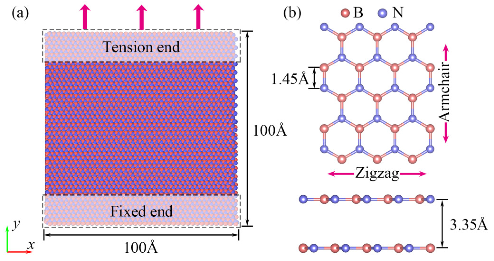
2.1. MDs Simulations

The mechanical properties of boron nitride nanosheets (BNNSs) were investigated through the simulation of over 300 sets of tensile cases using LAMMPS software [29]. The influence of various factors including the layer number, chirality, temperature, and tensile velocity on the mechanical behavior of BNNSs was examined. Figure 1 presents the uniaxial tensile simulation model and the structure of the BNNSs. The model possessed dimensions of 100 Å in length and width, with one end being fixed while the other end experienced tensile loading under a constant force. The BNNSs exhibited a hexagonal lattice structure characterized by lattice constants of 2.51 Å, 2.51 Å, and 6.69 Å. Two distinct chiralities were considered, namely, the zigzag and the armchair configurations. The B-N bond length was set to be 1.45 Å, while the interlayer spacing of the BNNSs in their initial state was 3.35 Å.

During the tensile molecular dynamics (MDs) simulation, an initial step involved the conjugate gradient energy minimization procedure. This step was carried out under specific conditions where the force and energy values were set at ${10}^{-17}$ kcal/(mol·Å) and ${10}^{-17}$ kcal/mol, respectively. Following the energy minimization, the BNNSs specimen underwent relaxation for a duration of 10 ps within the NPT ensemble. Then, additional relaxation occurred within the NVT ensemble, employing a 1 fs timestep, until the system achieved stability. Once the stable state was achieved, a uniaxial tensile load was applied along the y-axis to one end of the tensile model. This load was imposed at different but constant tensile velocities, while the other end of the model remained fixed. After the tensile deformation, a relaxation period of 5 ps was performed to attain a new equilibrium state for the composite specimen. Non-periodic boundary conditions were enforced for all the dimensions of the BNNS specimen, and the NVT ensemble was utilized for the tensile deformation simulation. To describe the interactions among the B-N, B-B, and N-N components within the BNNSs, the extended Tersoff (ExTeP) potential [30] was employed in the MDs simulation. Recently, a large number of MDs simulations using ExTeP potential have been used to research BN performance [31,32,33]. It is worth noting that the MDs simulation using BN ExTeP potential may not be as accurate as the results calculated ab initio. The parameters used for the BNNSs’ tensile simulation are summarized in

Table 1. Computational parameters used in the MDs simulations.

MDs Parameters	Value
Specimen material	BNNSs
Specimen dimensions (Å)	100 × 100
Chirality	Armchair, zigzag
Layer numbers	2, 3, 4, 5, 6
Ambient temperature (K)	1, 100, 200, 300, 500, 800
Tensile velocity (m/s)	10, 40, 70, 100, 200
Potential function	ExTeP
Timestep (fs)	1

.

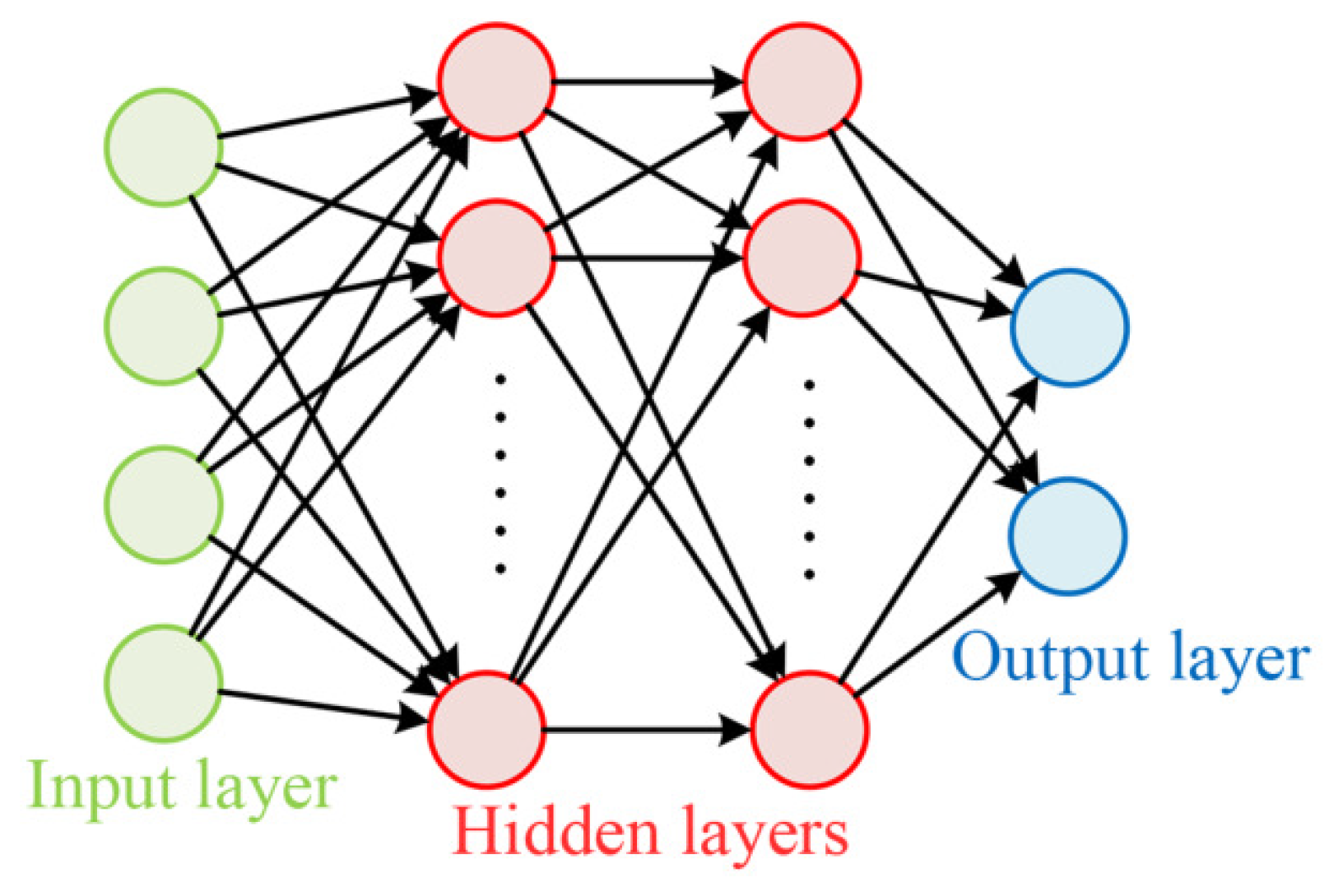
2.2. ML Prediction Models

The results of the MDs simulation were employed to train a variety of machine learning (ML) models, encompassing artificial neural networks (ANNs), support vector machines (SVMs), Boost regression, and random forest regression [34]. These models were constructed and optimized using the PyCharm software [35]. The ANN, a powerful ML technique, excels in addressing intricate nonlinear problems by predicting target variables based on input information [36]. For nonlinearly separable data, ANN models with two or more hidden layers exhibit enhanced regression performance. The architecture of the ANN consists of an input layer, one or two hidden layers, and an output layer, as shown in Figure 2. In this work, a feedforward neural network was employed for regression problem solving, where cyclic connections between neurons are absent. The input layer consists of four parameters: the number of layers, chirality, ambient temperature, and tensile velocity (v) of the BNNSs. The hidden layer comprises either one or two layers, each with 20, 30, or 40 neurons. The output layer is responsible for predicting the mechanical properties of the BNNSs, including the ultimate tensile strength and Young’s modulus. Information is transmitted through interconnected neurons from the input layer to the output layer, with the neurons in the hidden layers playing a pivotal role in mapping the input to the output [37]. This mapping can be represented as follows:

$$y\left(x\right)=f({\sum }_{\mathrm{i}=1}^{\mathrm{n}}{w}_{\mathrm{i}}{x}_{\mathrm{i}}+b)$$

(1)

where one of the neurons is assigned a bias value b and corresponding weights $w_{\mathrm{i}}$ for multiple inputs. The transfer function is denoted as f. Initially, the weights and biases are assigned random values. The training process involves continuously adjusting these weights and biases using a training set in order to minimize the mean square error (MSE). The hidden layer employs the sigmoid function as its transfer function, whereas the output layer utilizes a linear function. As a preventive measure against overfitting, the variation in the MSE during training is monitored, and the training process is stopped once this parameter ceases to decrease. Upon the completion of training, the accuracy of the ANN prediction is evaluated using the test set.

The SVM regression algorithm has proven to be a highly effective machine learning method for predicting the mechanical properties of materials [38]. Notably, the SVM has demonstrated superior performance in terms of both accuracy and computational efficiency when compared to other ML models [39]. This superiority can be attributed to the SVM’s ability to summarize norms using fewer feature data, as well as its avoidance of the iterative process involved in optimizing weights and biases in ANNs. The primary objective of the SVM is to identify a function that not only maximizes the margin but also ensures the data points lie as flatly as possible. Through iterative optimization, the SVM determines the optimal function, denoted as $y\left(x\right)$, for the training dataset. The predicted solution for an input vector $x_i$ is then obtained using the following equation [40]:

$$y\left(x\right)={\sum }_{\mathrm{i}=1}^{\mathrm{n}}{w}_{\mathrm{i}}K(x,x_{\mathrm{i}})+w_0$$

(2)

where $K(x,x_{\mathrm{i}})$ represents the kernel function, while $w_{\mathrm{i}}$ denotes the corresponding weighting parameter.

In this work, the SVM employed both linear and Gaussian kernel functions. The linear kernel, denoted as L-SVM, conducted regression by linearly transforming the input into a higher-dimensional feature space. In contrast, the Gaussian kernel, represented as G-SVM, achieved regression by nonlinearly mapping the input to the same feature space of high dimensionality. The Gaussian kernel function is given as follows:

$$K(x,\mathrm{i})=e^{-\frac{{∥x-x_{\mathrm{i}}∥}^2}{{\sigma }^2}}$$

(3)

where ${\sigma }^2$ represents the bandwidth of the Gaussian kernel.

The Boost algorithm, as proposed by Schapire in 2003 [41], is an ensemble technique that combines the predictions of multiple weak classifiers to construct a robust classifier. Through an iterative process, the algorithm utilizes new training data to enhance the performance achieved in the previous iteration, effectively avoiding overfitting. AdaBoost, short for Adaptive Boosting, is a specific variant of the Boost algorithm. This process entails boosting the weights of misclassified samples while reducing the weights of correctly classified samples. Following this, the modified weighted samples are used to train the next classifier, and this process continues until the error rate falls below a predefined threshold or reaches the maximum allowable number of iterations. AdaBoost’s adaptability is evident in its capacity to establish an upper bound without explicit specification, resulting in an exponential reduction in the loss function. In this work, the ultimate classifier in the AdaBoost algorithm can be expressed as [42]:

$$y\left(x\right)={\sum }_{\mathrm{m}=1}^{\mathrm{M}}{\alpha }_{\mathrm{m}}{G}_{\mathrm{m}}\left(x\right)$$

(4)

where $G_{\mathrm{m}}\left(x\right)$ represents the weak classifier obtained in the m iteration, and ${\alpha }_{\mathrm{m}}$ represents the weight of $G_{\mathrm{m}}\left(x\right)$ in the final classifier.

The eXtreme Gradient Boost (XGBoost) algorithm is a sophisticated distributed gradient boosting library meticulously engineered to possess qualities of efficiency, flexibility, and portability. It serves as a powerful framework for constructing large-scale parallel boosting trees, surpassing the speed of conventional toolkits by a factor of over ten. In our study, we employ the regression tree algorithm as the weak classifier within the XGBoost model. The predictive outcome of sample i following the mth iteration is mathematically denoted as [43]:

$${\widehat{y}}_{\mathrm{i}}^{\left(\mathrm{m}\right)}={\sum }_{\mathrm{k}=1}^{\mathrm{m}}{f}_{\mathrm{k}}\left(x_{\mathrm{i}}\right)={\widehat{y}}_{\mathrm{i}}^{(\mathrm{m}-1)}+f_{\mathrm{m}}\left(x_{\mathrm{i}}\right)$$

(5)

where ${\widehat{y}}_{\mathrm{i}}^{\left(\mathrm{m}\right)}$ denotes the prediction result obtained from the previous m-1 trees. $f_{\mathrm{m}}\left(x_{\mathrm{i}}\right)$ represents the function of the m-th tree, which is derived by solving the loss function through second-order Taylor expansion. This approach not only enhances prediction accuracy but also facilitates the customization of the loss function.

Random forest is a well-established ensemble learning technique that employs numerous decision trees for training, classifying, and predicting samples, primarily in regression and classification scenarios [44]. Its individual base learners function independently and can be executed concurrently. The algorithm is fundamentally based on decision trees. To begin, m samples are randomly selected with a replacement from the original dataset, creating m training sets. Subsequently, each training set is employed to train a decision tree, yielding m decision trees. The optimal feature for a single decision tree model is selected for partitioning. Ultimately, the generated decision trees are amalgamated to form a random forest. Given that this study addresses a regression problem, the final prediction outcome is determined by the mean of the predicted values derived from multiple trees.

2.3. Data Prediction

Using MDs simulations, we identified four key factors influencing the material’s ultimate tensile strength and Young’s modulus. We employed machine learning techniques to establish the significance-based ranking of these factors. Given the challenges in crafting expressions to depict the impact of the BNNSs’ chirality on the ultimate tensile strength and Young’s modulus, our discussions were centered on two specific chiralities. Notably, the fitting formula maintained a consistent structure, regardless of chirality. The fitting process and subsequent results’ evaluation were carried out using PyCharm software. The predictive models for the ultimate tensile strength and Young’s modulus of the BNNSs are presented below:

$$U=(a_{1}n+a_{2}v+a_3){\mathrm{e}}^{a_{4}T}$$

(6)

$$E=(b_{1}n+b_2){\mathrm{e}}^{b_{3}T}ln(v+b_4)$$

(7)

where n represents the total number of layers, v denotes the velocity of the tensile loading, T signifies the ambient temperature, $a_{\mathrm{i}}$ and $b_{\mathrm{i}}$ (where i = 1, 2, 3, 4) correspond to the coefficients, U indicates the predicted values of the ultimate tensile strength, and E represents the predicted values of Young’s modulus.

3. Results and Discussions

The U and E of the multilayer BNNSs were determined through MDs simulations. E is obtained by calculating the slope of the front 1% of the stress–strain curve using the least square method, where U is the stress corresponding to the highest peak of the stress–strain curve. Each of the 300 groups’ E and U were obtained by averaging five different random initial atomic velocity systems. Our findings demonstrate that the stress–strain relationship exhibits linearity at low strains, employing Hooke’s law, consistent with the observations made by Guo et al. [45] during their uniaxial tensile test. The MDs simulation results serve as input for the ML models to predict various outcomes. For the same input conditions, the difference in the MDs simulation results does not exceed 2%, and the difference in the ML prediction results does not exceed 5%.

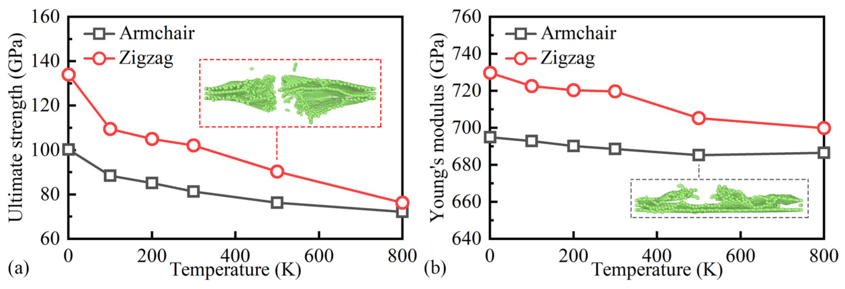
3.1. Influence of Temperature

Figure 3 shows the stress–strain curves with three layers of BNNSs at various temperatures under a tensile velocity of 10 m/s. The stress–strain relationship exhibits nearly linear behavior during the elastic regime, irrespective of the temperature. Upon reaching the ultimate tensile position, the curve exhibits a sharp decline attributed to the rupture of the chemical bonds between the B and N atoms within a single layer, signifying the onset of plastic deformation in the BNNSs. Subsequently, the remaining two layers undergo rapid separation.

Figure 4 illustrates the behavior of the BNNSs with three layers under v = 10 m/s at different temperatures, focusing on the U and E. As depicted in Figure 4a, when the temperature increases from 1 K to 800 K, the U of the armchair and zigzag configurations decreases by 28% and 41%, respectively. Moreover, the U in the zigzag direction is 133% (at 1 K) and 105% (at 800 K) of that in the armchair direction. In Figure 4b, while the change in E with the temperature is less than 4% for the armchair orientation, both chiralities exhibit a decrease in E with an increasing temperature. These findings from Figure 4 support the softening effect of heating on the BNNSs, consistent with previous research [46,47,48]. Additionally, irrespective of the temperature, the U and E are higher in the zigzag direction compared to the armchair direction, indicating the presence of mechanical anisotropy in the BNNSs.

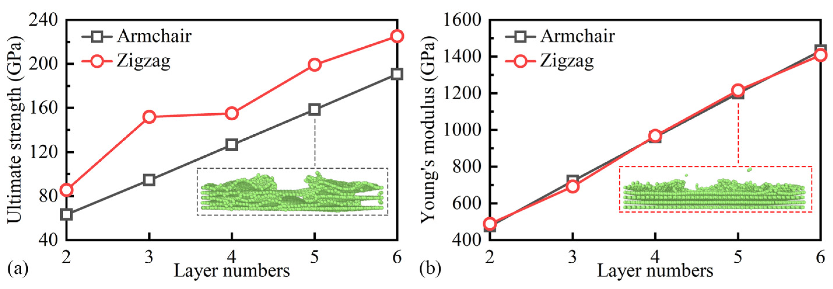
3.2. Effect of Layer Numbers

The stress–strain curves for the armchair and zigzag orientations at 300 K and v = 10 m/s, corresponding to different layer numbers, are depicted in Figure 5. Figure 5a,b demonstrate that the slope of the stress–strain curve increases incrementally with each additional layer, exhibiting a similar trend. Irrespective of the layer count, the U remains consistent in both directions. Notably, the U is found to be the lowest at five layers, potentially due to fortuitous factors. Furthermore, when the layer count is held constant, the E of the BNNSs is marginally higher in the zigzag direction compared to the armchair direction. For instance, the E for six-layer BNNSs in the zigzag and armchair directions is 592 GPa and 538 GPa, respectively, indicating a discrepancy of approximately 10%. The E of two layers of BNNSs in the zigzag and armchair direction is 195 GPa and 185 GPa, with a difference of about 5%.

Figure 6 illustrates the variations in U and E of the BNNSs across different layer configurations, ranging from two to six layers, at a temperature of 300 K and v of 10 m/s. As depicted in Figure 6a, it is evident that the value of U exhibits an upward trend as the temperature increases. Furthermore, it can be observed that the U in the zigzag direction surpasses that in the armchair direction for all the layer configurations. Specifically, the U values for the three-layer BNNSs amount to 155.1 GPa (zigzag) and 126.2 GPa (armchair), signifying a 23% difference. Moving on to Figure 6b, a linear relationship between E and the number of layers is clearly evident. The E values in the zigzag and armchair directions are nearly identical, aligning with the findings obtained from the calculations presented in Figure 5. Hence, these outcomes indicate the anisotropic nature of the BNNSs in terms of U and their weak nature with respect to E.

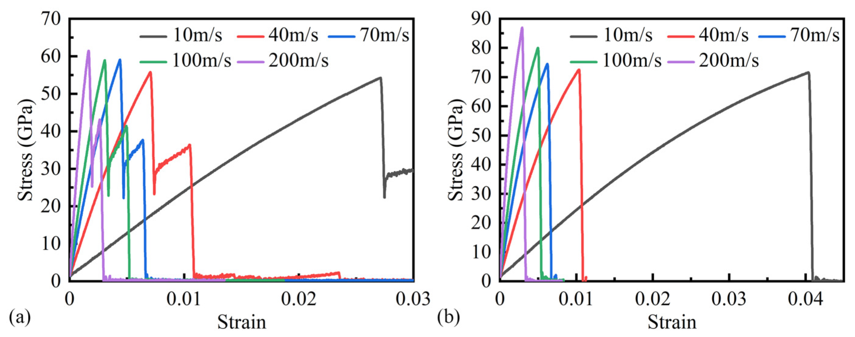
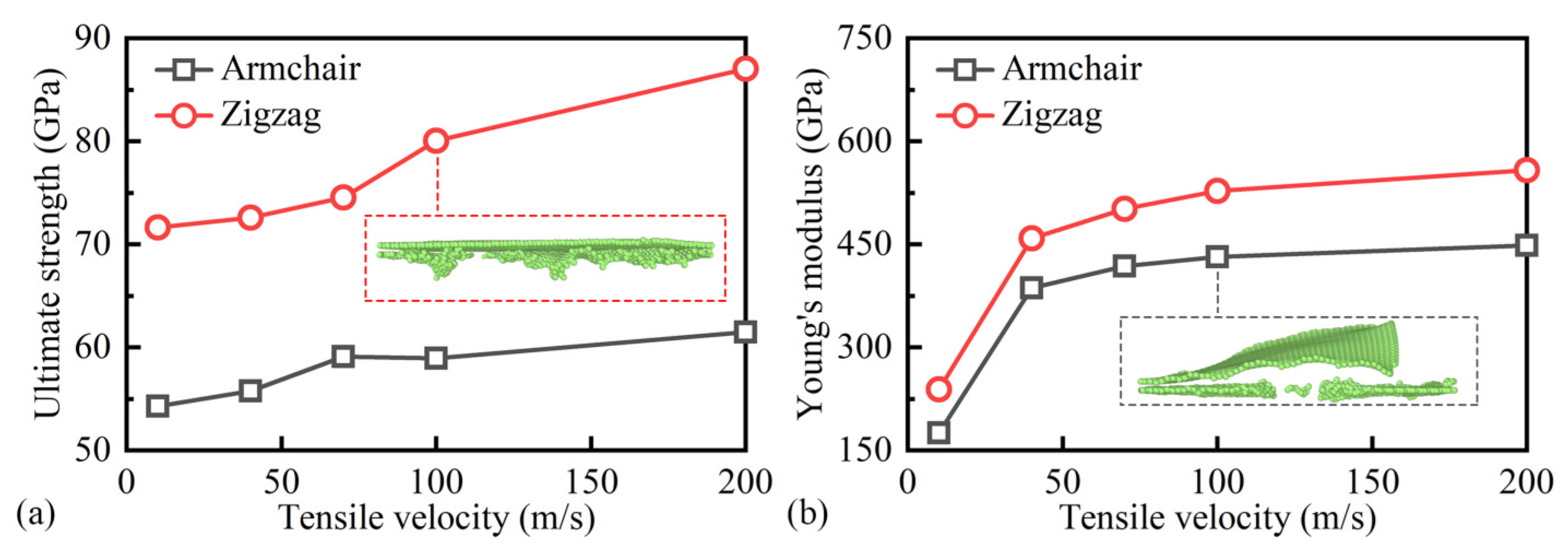
3.3. Effect of Tensile Velocity

Figure 7 illustrates the stress–strain behaviors of the two-layer BNNSs in the armchair and zigzag directions at a temperature of 300 K, under varying tensile velocities. By comparing the stress–strain curves depicted in Figure 7a,b, it is observed that the successive fracture of the two layers of BNNSs occurs in the case of the armchair structure, whereas the two layers with the zigzag structure experience simultaneous destruction. These findings indicate that the U decreases while the E increases as the tensile velocity increases, irrespective of the directions being armchair or zigzag. It is similar to the results reported by Han et al. [49] through MDs simulation.

Figure 8 illustrates the variations in the magnitudes of U and E for the two-layer BNNSs at a temperature of 300 K with different tensile velocities from 10 m/s to 200 m/s. As depicted in Figure 8a, there is an increase in U as the tensile velocity rises. Notably, the U values for v = 70 m/s and v = 100 m/s along the armchair direction are nearly equal, amounting to 58.9 GPa. However, as the tensile velocity surpasses 70 m/s, the discrepancy between the U values in the two directions increases, transitioning from 15 GPa (v = 10 m/s) to 26 GPa (v = 10 m/s). In Figure 8b, E exhibits a similar increasing trend with the tensile velocity, albeit with a diminishing growth rate. At a velocity of v = 40 m/s, E in the zigzag direction exceeds that in the armchair direction by 58 GPa. Nonetheless, when the tensile velocity reaches 200 m/s, the disparity in E between the two orientations is merely 20 GPa.

From Figure 4, Figure 6, and Figure 8, it can be observed that the BNNSs demonstrate superior mechanical characteristics in the zigzag orientation compared to the armchair orientation. In general, the tensile strength of the zigzag BNNSs is higher, aligning with other studies on chirality [46,50,51].

3.4. Modeling with ML

The previous research indicates that the values of E and U in multilayer BNNSs are primarily influenced by factors, such as the temperature, layer numbers, tensile velocity, and chirality. Prior to performing the ML modeling, a comprehensive dataset comprising more than 300 data points was generated through the MDs simulations. In these simulations, the temperature, layer number, tensile velocity, and chirality were considered as the input parameters, while U and E served as the output parameters. To facilitate the training of the ANN, AdaBoost, XGBoost, SVM, and random forest models, the dataset was randomly divided into two subsets: the training set, which encompassed 80% of the data, and the testing set, which comprised the remaining 20% of the data.

There are six different ANNs, with each hidden layer consisting of twenty, thirty, and forty neurons. The ANNs of three single-hidden layers are represented by ANN-20, ANN-30, and ANN-40. Correspondingly, the ANNs of the three double-layer hidden layers are represented by ANN-20-20, ANN-30-30, and ANN-40-40. The neurons in the input layer correspond to four influence factors, while the output layer contains two neurons dedicated to prediction. For the effective prediction of the U and E values in the BNNSs, it is crucial to incorporate an adequate number of neurons in the hidden layer to optimize the mapping process and attain superior output. However, an excessively large number of neurons in the hidden layer may result in overfitting and prolonged training times, leading to significant deviations in the projected outcomes. To mitigate the overall model loss, the Levenberg–Marquardt algorithm is employed as the solver. The logistic sigmoid function acts as the activation function for the hidden layer nodes, with a maximum iteration limit set at 10,000. Following the training of the ANN model, input test data are utilized for prediction purposes. Figure 9 and Figure 10 visually illustrate the correlation between the predicted values and test values for the single-layer and double-layer ANN models separately. The solid black line signifies the ideal prediction outcome, while the variance between the data points and the solid black line reflects the level of inaccuracy in the corresponding test value predictions.

Two Boost models, namely AdaBoost and XGBoost, were employed in this work. The learning rate and the number of weak evaluators in the AdaBoost model were adjusted to minimize the mean square error. Similarly, fine-tuning was performed on the learning rate, the number of weak evaluators, and the penalty coefficient gamma in the XGBoost model, optimizing the process based on the minimum mean squared error. Additionally, two SVM models, denoted as G-SVM and L-SVM, utilizing Gaussian and linear kernels, were chosen. The hyperparameters were adjusted using the grid algorithm to minimize the mean squared error. For L-SVM, the hyperparameters included the penalty parameter C and the radius of the insensitive region $ϵ$. The G-SVM model, in addition to these parameters, incorporated the kernel coefficient $\gamma$. Concerning the random forest model, the parameter optimized was the number of weak estimators, achieved by minimizing the minimum mean squared error. During the training phase, 80% of the available data was randomly utilized, with the remaining 20% was reserved for testing. Regression plots illustrating the predicted values of U and E by the Boost, SVM, and random forest models are presented in Figure 11, Figure 12, and Figure 13, respectively.

When employing ML techniques to address regression problems, the evaluation of the model performance entails the utilization of metrics, such as the mean squared error (MSE) and the coefficient of determination ($R^2$). The MSE is recognized as a pivotal criterion for assessing performance, wherein smaller values indicate a higher degree of accuracy exhibited by the model. Conversely, $R^2$, widely adopted as a parameter for gauging ML model effectiveness, signifies the correlation between the predicted and actual values of the model. Ranging from 0 to 1, values approaching 1 signify the heightened accuracy of the model. The computation of the MSE and $R^2$ is accomplished through Equations (8) and (9), respectively.

$$MSE=\frac{1}{n}{\sum }_{i=1}^n{(y_i-{\widehat{y}}_i)}^2$$

(8)

$$R^2=1-\frac{{\sum }_{i=1}^n{(y_i-{\widehat{y}}_i)}^2}{{\sum }_{i=1}^n{(y_i-\overline{y})}^2}$$

(9)

where $y_i$ denotes the actual value, ${\widehat{y}}_i$ denotes the estimated value, $\overline{y}$ signifies the average of the estimated values, and n represents the total sample count.

Table 2. The MSE and $R^2$ of different models for U.

ML Models	MSE	${\mathit{R}}^2$
ANN-20	39.094	0.9792
ANN-30	37.481	0.9808
ANN-40	35.059	0.9867
ANN-20-20	36.151	0.9852
ANN-30-30	32.659	0.9887
ANN-40-40	34.907	0.9873
AdaBoost	214.98	0.9287
XGBoost	75.559	0.9746
G-SVM	456.86	0.8467
L-SVM	275.45	0.9077
Random Forest	32.644	0.9889

and

Table 3. The MSE and $R^2$ of different models for E.

ML Models	MSE	${\mathit{R}}^2$
ANN-20	14502	0.8857
ANN-30	14463	0.8860
ANN-40	16190	0.8682
ANN-20-20	12663	0.9089
ANN-30-30	12326	0.9164
ANN-40-40	13501	0.8971
AdaBoost	26867	0.7883
XGBoost	18786	0.8520
G-SVM	20818	0.8360
L-SVM	29469	0.7678
Random Forest	11095	0.9215

exhibit the MSE and $R^2$ values achieved by the various models following the training to forecast the values of U and E. Figure 14 displays the $R^2$ values pertaining to the prediction of U and E. Table 2 and Figure 14a demonstrate that the double-layer artificial neural network (ANN) model exhibits a slightly superior performance compared to the single-layer ANN model in the prediction of U. For instance, the MSE and $R^2$ values for the ANN-40 model are recorded as 35.059 and 0.9867, respectively, while for the ANN-40-40 model, they are reported as 34.907 and 0.9873. However, the observed enhancement remains marginal in nature.

Moreover, the performance differences between the three single-layer ANN models and the three double-layer ANN models were insignificant. The MSE and $R^2$ of AdaBoost were found to be higher compared to those of XGBoost, suggesting that XGBoost outperforms AdaBoost in terms of accuracy and consistency. Likewise, in the SVM models, L-SVM demonstrated superior performance to G-SVM in the metric of U. However, both the Boost and SVM models exhibited inferior performance compared to the other six ANN models. Among these models, the random forest model demonstrated the smallest MSE and its $R^2$ value was close to 1, indicating its superior predictive performance for the variable U.

From Table 3 and Figure 14b, it is observed that augmenting the quantity of neurons in the concealed layer might not significantly enhance the performance of the model. It is evident that in the case of a single-layer ANN model, amplifying the number of neurons in the hidden layer actually results in a decline in the model’s performance, with ANN-40 exhibiting poor performance. Among all the ANN models, the performance of ANN-30-30 is the most favorable. In the two Boost models, XGBoost surpasses AdaBoost in predicting U as well. Nevertheless, in the SVM, G-SVM outperforms L-SVM in predicting E. Among these models, random forest also demonstrates the superior performance in predicting E.

The aforementioned analysis indicates that the random forest model is the optimal choice for predicting the dataset. This model possesses a parameter known as feature importance (FI), which provides quantitative contributions of four parameters toward U and E.

Table 4. The FI of parameters to U and E.

Parameters	U	E
Chirality	0.112	0.026
Number of layers	0.728	0.797
Ambient temperature	0.141	0.099
Tensile velocity	0.019	0.077

exhibits the FI values associated with the chirality, layer count, temperature, and tensile velocity concerning U and E correspondingly. It is evident that the layer count emerges as the most influential factor affecting both U and E. Conversely, the impact of the tensile velocity on U is negligible, while the chirality of the BNNSs has a minor influence on E.

3.5. Prediction Models

A numerical fitting approach was employed to establish a prediction model for the variables U and E. The equations representing the formulas for U in the case of the armchair and zigzag chiralities are denoted as Equation (10) correspondingly.

$$\left\{\begin{array}{c}{U}_{\mathrm{A}}=(32.380n+3.6753v-0.82602){\mathrm{e}}^{-0.00035942T}\\ U_{\mathrm{Z}}=(40.075n+8.5374v+3.5182){\mathrm{e}}^{-0.00046614T}\end{array}\right.$$

(10)

The E formulas for the armchair and zigzag chiralities are as follows:

$$\left\{\begin{array}{c}{E}_{\mathrm{A}}=(96.354n-2.8069){\mathrm{e}}^{-0.00015554T}ln(v+11.136)\\ E_{\mathrm{Z}}=(36.808n+10.903){\mathrm{e}}^{-0.0000070361T}ln(v+351.50)\end{array}\right.$$

(11)

Table 5. The MSE and $R^2$ for U and E prediction.

Prediction Models	MSE	${\mathit{R}}^2$
$U_{\mathrm{A}}$ equation	25.458	0.9863
$U_{\mathrm{Z}}$ equation	82.627	0.9715
$E_{\mathrm{A}}$ equation	12714	0.8924
$E_{\mathrm{Z}}$ equation	14030	0.8745

presents the MSE and $R^2$ of the prediction model applied to the variables U and E. In addition, the mean absolute errors (MAEs) of $U_{\mathrm{A}}$ and $U_{\mathrm{Z}}$ are 3.3917 GPa and 7.0802 GPa, respectively. The MAEs of $E_{\mathrm{A}}$ and $E_{\mathrm{Z}}$ are 66.599 GPa and 79.452 GPa, respectively. The results indicate that the performance of the prediction model is comparable to that of the majority of the ML models, albeit less precise than the random forest model. Nonetheless, this prediction model can serve as a valuable point of reference for future investigations.

4. Conclusions

A practical approach for estimating the E and U of the BNNSs using MDs simulations and ML models has been introduced. This study investigates the effects of the chirality, layer number, ambient temperature, and tensile velocity on the mechanical behavior of BNNSs. Multiple ML models are trained based on over 300 sets of MDs simulation data, and the random forest model is selected as the optimal choice for accurately predicting the mechanical properties of the BNNSs. By employing this model, the time-consuming MDs simulations for the BNNSs can be significantly reduced. The findings of this research demonstrate the following:

(1)

The integration of MDs simulations and ML techniques offers a precise and reliable approach for predicting the mechanical properties of BNNSs. This proposed methodology can be readily extended to forecast other properties of BNNSs as well as those of other two-dimensional nanomaterials.

(2)

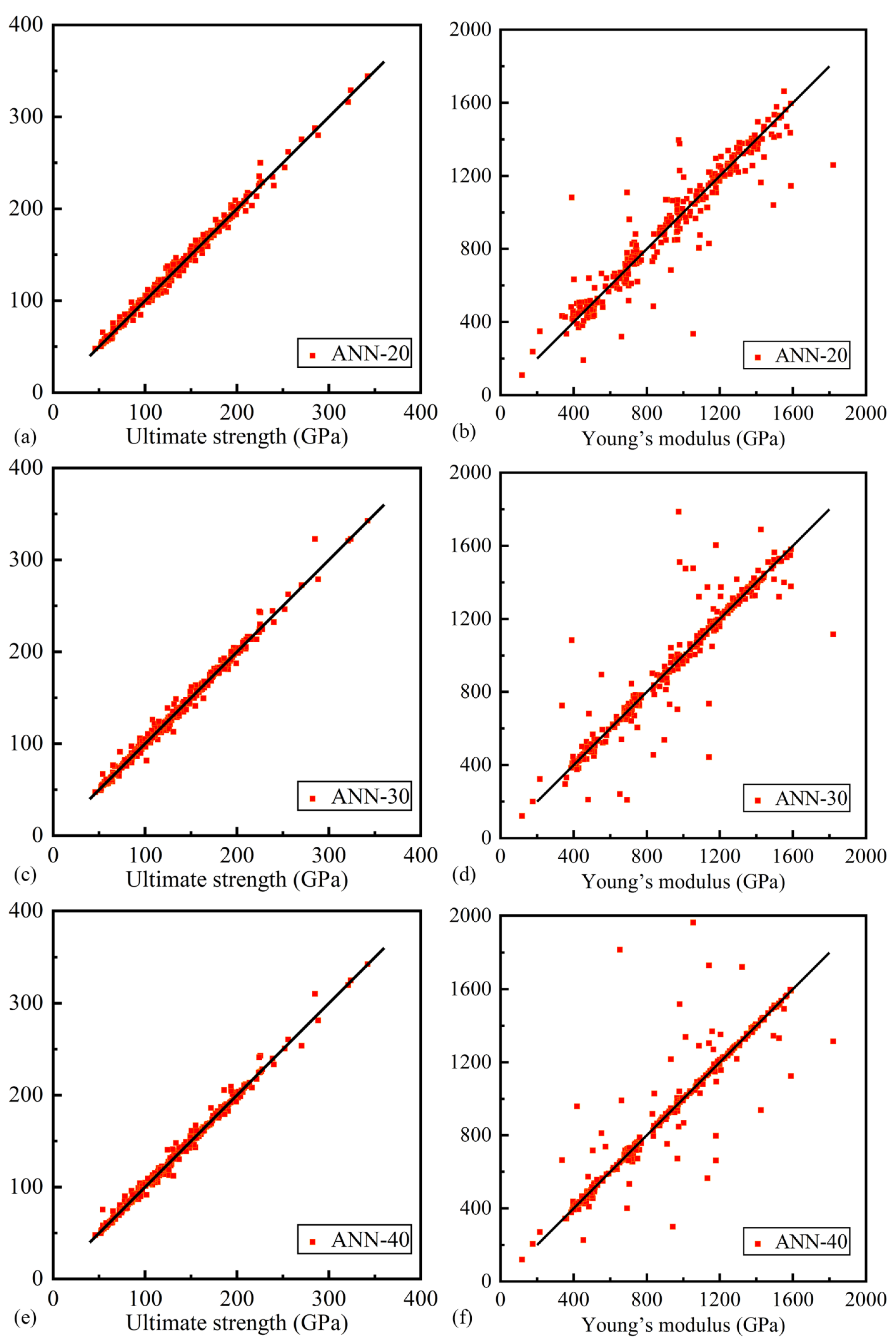
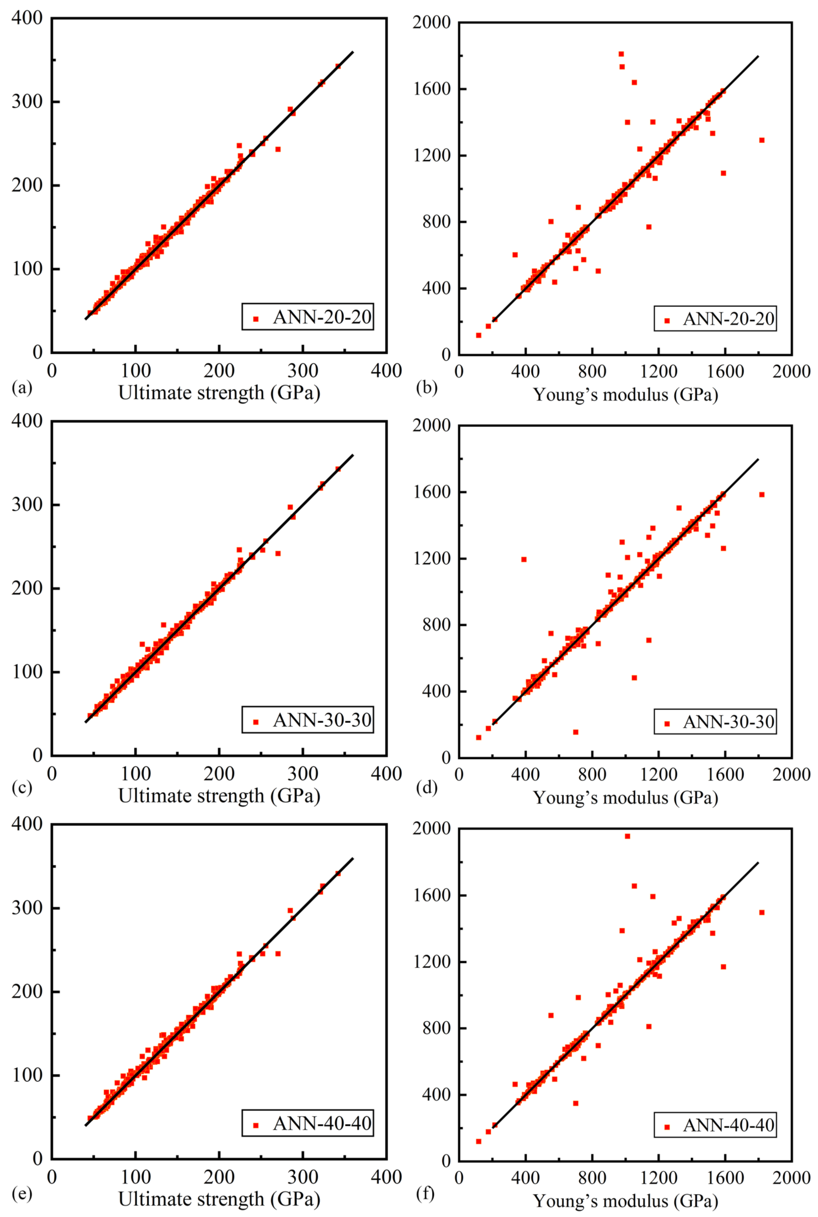
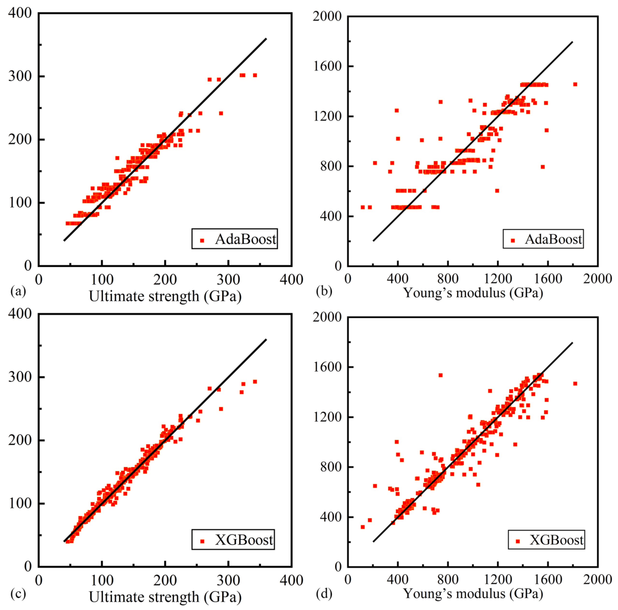
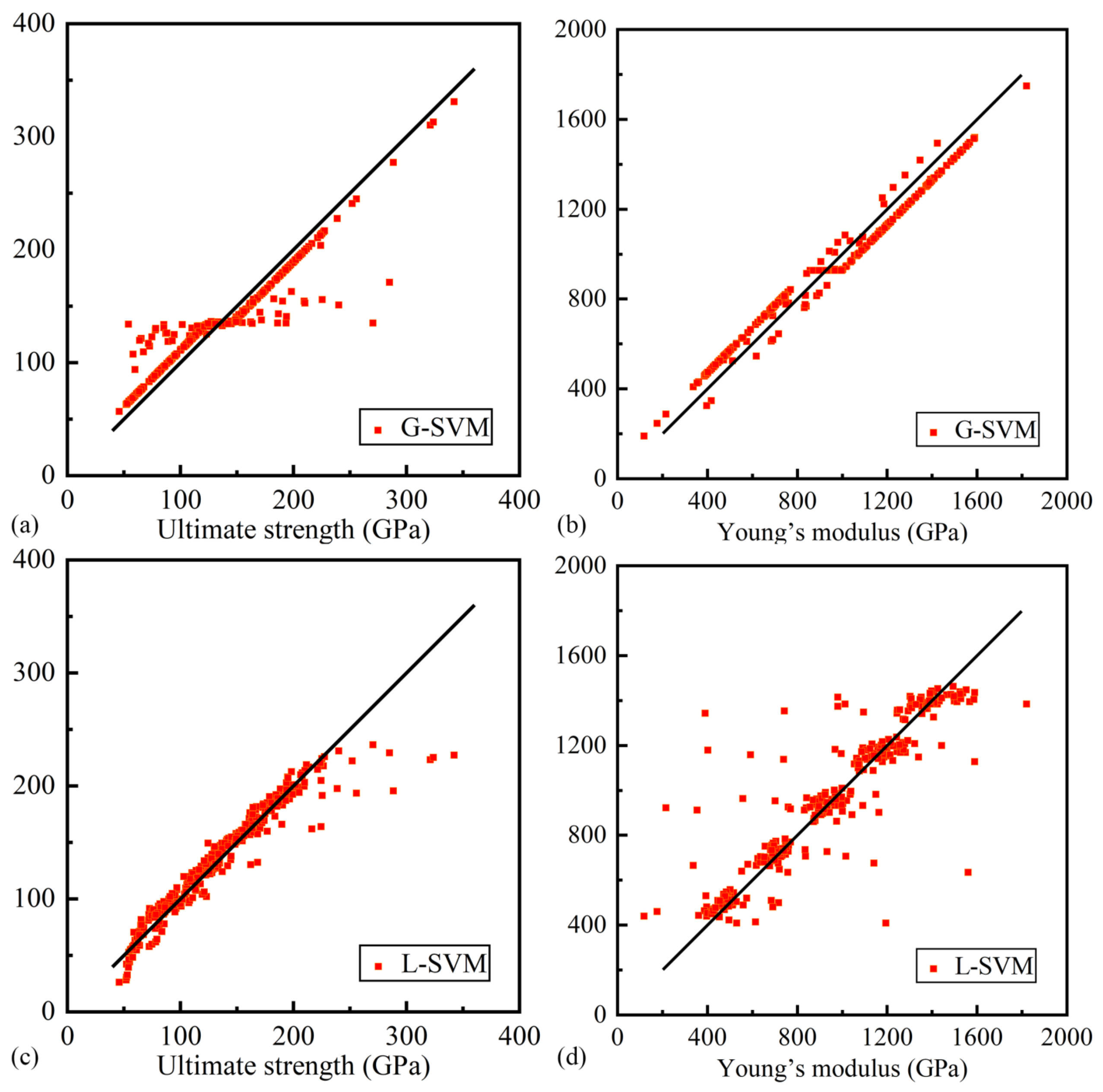
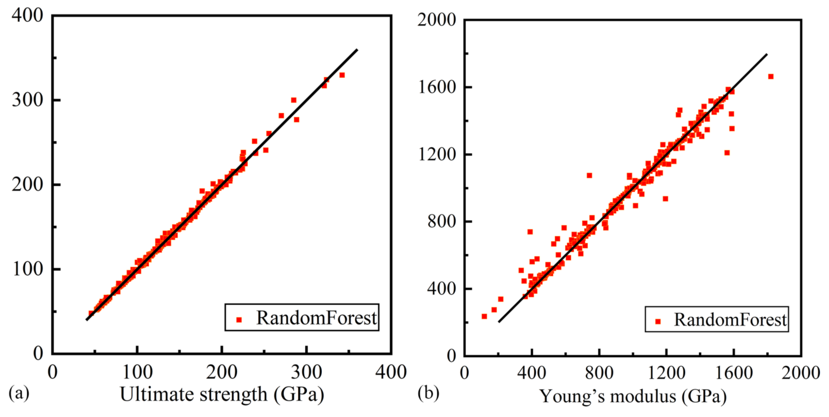
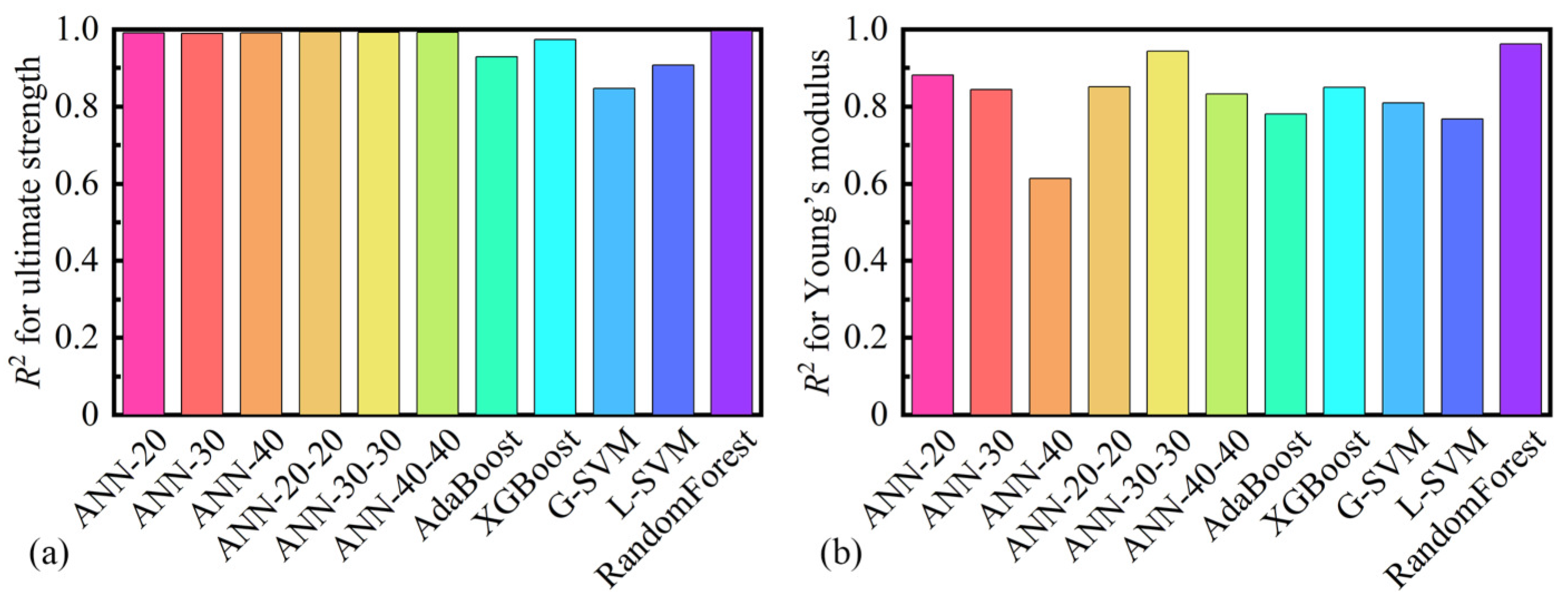
Several ML models are trained and evaluated, revealing that the random forest model performs exceptionally well in predicting the mechanical properties of BNNSs. The ANN model accurately predicts the U, but its performance in predicting the E varies among the different ANN models, resulting in challenges in achieving accurate predictions. The XGBoost model yields more accurate predictions for U but shows poor performance in predicting E. On the other hand, the AdaBoost, G-SVM, and L-SVM models exhibit limited accuracy in predicting the mechanical properties.

(3)

The feature importance analysis of the random forest model indicates that the layer number has the most significant influence on both the U and E of the BNNSs. In contrast, the chirality of the BNNSs has a negligible impact on U, while the tensile velocity has a minor effect on E.

(4)

Based on the combined findings from the MDs simulations and ML models, a predictive model for estimating the U and E of the BNNSs is proposed. The two different chiralities are numerically fitted, and the MSE and $R^2$ values of the prediction models are calculated. The results indicate that the prediction accuracy of this model is comparable to that of the ANN models, thereby offering valuable insights for future research endeavors.

References

1. Gupta, A.; Sakthivel, T.; Seal, S. Recent development in 2D materials beyond graphene. Prog. Mater. Sci. 2015, 73, 44–126. [Google Scholar] [CrossRef]
2. Bao, J.; Jeppson, K.; Edwards, M.; Fu, Y.; Ye, L.; Lu, X.; Liu, J. Synthesis and applications of two-dimensional hexagonal boron nitride in electronics manufacturing. Electron. Mater. Lett. 2016, 12, 1–16. [Google Scholar] [CrossRef]
3. Watanabe, K.; Taniguchi, T.; Kanda, H. Direct-bandgap properties and evidence for ultraviolet lasing of hexagonal boron nitride single crystal. Nat. Mater. 2004, 3, 404–409. [Google Scholar] [CrossRef] [PubMed]
4. Zhang, D.L.; Zha, J.W.; Li, C.Q.; Li, W.K.; Wang, S.J.; Wen, Y.; Dang, Z.M. High thermal conductivity and excellent electrical insulation performance in double-percolated three-phase polymer nanocomposites. Compos. Sci. Technol. 2017, 144, 36–42. [Google Scholar] [CrossRef]
5. Zhi, C.; Bando, Y.; Tang, C.; Kuwahara, H.; Golberg, D. Large-scale fabrication of boron nitride nanosheets and their utilization in polymeric composites with improved thermal and mechanical properties. Adv. Mater. 2009, 21, 2889–2893. [Google Scholar] [CrossRef]
6. Li, J.; Gui, G.; Zhong, J. Tunable bandgap structures of two-dimensional boron nitride. J. Appl. Phys. 2008, 104, 094311. [Google Scholar] [CrossRef]
7. Ishida, H.; Rimdusit, S. Very high thermal conductivity obtained by boron nitride-filled polybenzoxazine. Thermochim. Acta 1998, 320, 177–186. [Google Scholar] [CrossRef]
8. Guerra, V.; Wan, C.; McNally, T. Thermal conductivity of 2D nano-structured boron nitride (BN) and its composites with polymers. Prog. Mater. Sci. 2019, 100, 170–186. [Google Scholar] [CrossRef]
9. Kostoglou, N.; Polychronopoulou, K.; Rebholz, C. Thermal and chemical stability of hexagonal boron nitride (h-BN) nanoplatelets. Vacuum 2015, 112, 42–45. [Google Scholar] [CrossRef]
10. Golberg, D.; Bando, Y.; Huang, Y.; Terao, T.; Mitome, M.; Tang, C.; Zhi, C. Boron nitride nanotubes and nanosheets. ACS Nano 2010, 4, 2979–2993. [Google Scholar] [CrossRef]
11. Chen, J.; Huang, X.; Sun, B.; Jiang, P. Highly thermally conductive yet electrically insulating polymer/boron nitride nanosheets nanocomposite films for improved thermal management capability. ACS Nano 2018, 13, 337–345. [Google Scholar] [CrossRef] [PubMed]
12. Ismach, A.; Chou, H.; Ferrer, D.A.; Wu, Y.; McDonnell, S.; Floresca, H.C.; Covacevich, A.; Pope, C.; Piner, R.; Kim, M.J.; et al. Toward the controlled synthesis of hexagonal boron nitride films. ACS Nano 2012, 6, 6378–6385. [Google Scholar] [CrossRef] [PubMed]
13. Shi, Y.; Hamsen, C.; Jia, X.; Kim, K.K.; Reina, A.; Hofmann, M.; Hsu, A.L.; Zhang, K.; Li, H.; Juang, Z.Y.; et al. Synthesis of few-layer hexagonal boron nitride thin film by chemical vapor deposition. Nano Lett. 2010, 10, 4134–4139. [Google Scholar] [CrossRef] [PubMed]
14. Song, L.; Ci, L.; Lu, H.; Sorokin, P.B.; Jin, C.; Ni, J.; Kvashnin, A.G.; Kvashnin, D.G.; Lou, J.; Yakobson, B.I.; et al. Large scale growth and characterization of atomic hexagonal boron nitride layers. Nano Lett. 2010, 10, 3209–3215. [Google Scholar] [CrossRef] [PubMed]
15. Kim, S.M.; Hsu, A.; Park, M.H.; Chae, S.H.; Yun, S.J.; Lee, J.S.; Cho, D.H.; Fang, W.; Lee, C.; Palacios, T.; et al. Synthesis of large-area multilayer hexagonal boron nitride for high material performance. Nat. Commun. 2015, 6, 8662. [Google Scholar] [CrossRef] [PubMed]
16. Ohba, N.; Miwa, K.; Nagasako, N.; Fukumoto, A. First-principles study on structural, dielectric, and dynamical properties for three BN polytypes. Phys. Rev. B 2001, 63, 115207. [Google Scholar] [CrossRef]
17. Peng, Q.; Ji, W.; De, S. Mechanical properties of the hexagonal boron nitride monolayer: Ab initio study. Comput. Mater. Sci. 2012, 56, 11–17. [Google Scholar] [CrossRef]
18. Mirnezhad, M.; Ansari, R.; Rouhi, H. Mechanical properties of multilayer boron nitride with different stacking orders. Superlattices Microstruct. 2013, 53, 223–231. [Google Scholar] [CrossRef]
19. Natsuki, T.; Natsuki, J. Prediction of mechanical properties for hexagonal boron nitride nanosheets using molecular mechanics model. Appl. Phys. A 2017, 123, 283. [Google Scholar] [CrossRef]
20. Han, G.; Zhang, D.; Kong, C.; Zhou, B.; Shi, Y.; Feng, Y.; Liu, C.; Wang, D.Y. Flexible, thermostable and flame-resistant epoxy-based thermally conductive layered films with aligned ionic liquid-wrapped boron nitride nanosheets via cyclic layer-by-layer blade-casting. Chem. Eng. J. 2022, 437, 135482. [Google Scholar] [CrossRef]
21. Mortazavi, B.; Rémond, Y. Investigation of tensile response and thermal conductivity of boron-nitride nanosheets using molecular dynamics simulations. Phys.-Low-Dimens. Syst. Nanostruct. 2012, 44, 1846–1852. [Google Scholar] [CrossRef]
22. Salavati, M.; Mojahedin, A.; Shirazi, A.H.N. Mechanical responses of pristine and defective hexagonal boron-nitride nanosheets: A molecular dynamics investigation. Front. Struct. Civ. Eng. 2020, 14, 623–631. [Google Scholar] [CrossRef]
23. Ding, Q.; Ding, N.; Liu, L.; Li, N.; Wu, C.M.L. Investigation on mechanical performances of grain boundaries in hexagonal boron nitride sheets. Int. J. Mech. Sci. 2018, 149, 262–272. [Google Scholar] [CrossRef]
24. Jin, K.; Luo, H.; Wang, Z.; Wang, H.; Tao, J. Composition optimization of a high-performance epoxy resin based on molecular dynamics and machine learning. Mater. Des. 2020, 194, 108932. [Google Scholar] [CrossRef]
25. Pan, S.; Wang, Y.; Yu, J.; Yang, M.; Zhang, Y.; Wei, H.; Chen, Y.; Wu, J.; Han, J.; Wang, C.; et al. Accelerated discovery of high-performance Cu-Ni-Co-Si alloys through machine learning. Mater. Des. 2021, 209, 109929. [Google Scholar] [CrossRef]
26. Moghadam, P.Z.; Rogge, S.M.; Li, A.; Chow, C.M.; Wieme, J.; Moharrami, N.; Aragones-Anglada, M.; Conduit, G.; Gomez-Gualdron, D.A.; Van Speybroeck, V.; et al. Structure-mechanical stability relations of metal-organic frameworks via machine learning. Matter 2019, 1, 219–234. [Google Scholar] [CrossRef]
27. Amani, M.A.; Ebrahimi, F.; Dabbagh, A.; Rastgoo, A.; Nasiri, M.M. A machine learning-based model for the estimation of the temperature-dependent moduli of graphene oxide reinforced nanocomposites and its application in a thermally affected buckling analysis. Eng. Comput. 2021, 37, 2245–2255. [Google Scholar] [CrossRef]
28. Liu, J.; Zhang, Y.; Zhang, Y.; Kitipornchai, S.; Yang, J. Machine learning assisted prediction of mechanical properties of graphene/aluminium nanocomposite based on molecular dynamics simulation. Mater. Des. 2022, 213, 110334. [Google Scholar] [CrossRef]
29. Plimpton, S. Fast parallel algorithms for short-range molecular dynamics. J. Comput. Phys. 1995, 117, 1–19. [Google Scholar] [CrossRef]
30. Los, J.H.; Kroes, J.M.H.; Albe, K.; Gordillo, R.M.; Katsnelson, M.I.; Fasolino, A. Extended Tersoff potential for boron nitride: Energetics and elastic properties of pristine and defective h-BN. Phys. Rev. B 2017, 96, 184108. [Google Scholar] [CrossRef]
31. Thiemann, F.L.; Rowe, P.; Muller, E.A.; Michaelides, A. Machine learning potential for hexagonal boron nitride applied to thermally and mechanically induced rippling. J. Phys. Chem. C 2020, 124, 22278–22290. [Google Scholar] [CrossRef]
32. Zhou, M.; Liang, T.; Wu, B.; Liu, J.; Zhang, P. Phonon transport in antisite-substituted hexagonal boron nitride nanosheets: A molecular dynamics study. J. Appl. Phys. 2020, 128, 234304. [Google Scholar] [CrossRef]
33. Shepelev, I.; Chetverikov, A.; Dmitriev, S.; Korznikova, E. Shock waves in graphene and boron nitride. Comput. Mater. Sci. 2020, 177, 109549. [Google Scholar] [CrossRef]
34. Mitchell, T.M. Machine Learning; McGraw-Hill: New York, NY, USA, 2007; Volume 1. [Google Scholar]
35. Zhou, X.; Zhao, J.; Chen, M.; Zhao, G.; Wu, S. Influence of catalyst and solvent on the hydrothermal liquefaction of woody biomass. Bioresour. Technol. 2022, 346, 126354. [Google Scholar] [CrossRef] [PubMed]
36. Kalogirou, S.A. Artificial neural networks in renewable energy systems applications: A review. Renew. Sustain. Energy Rev. 2001, 5, 373–401. [Google Scholar] [CrossRef]
37. Rojas, R. Neural Networks: A Systematic Introduction; Springer Science & Business Media: Berlin/Heidelberg, Germany, 2013. [Google Scholar]
38. Cortes, C.; Vapnik, V. Support-vector networks. Mach. Learn. 1995, 20, 273–297. [Google Scholar] [CrossRef]
39. Otchere, D.A.; Ganat, T.O.A.; Gholami, R.; Ridha, S. Application of supervised machine learning paradigms in the prediction of petroleum reservoir properties: Comparative analysis of ANN and SVM models. J. Pet. Sci. Eng. 2021, 200, 108182. [Google Scholar] [CrossRef]
40. Sobhani, J.; Khanzadi, M.; Movahedian, A. Support vector machine for prediction of the compressive strength of no-slump concrete. Comput. Concr. 2013, 11, 337–350. [Google Scholar] [CrossRef]
41. Schapire, R.E. The boosting approach to machine learning: An overview. In Nonlinear Estimation and Classification; Springer: Berlin/Heidelberg, Germany, 2003; pp. 149–171. [Google Scholar]
42. Friedman, J.H. Greedy function approximation: A gradient boosting machine. Ann. Stat. 2001, 29, 1189–1232. [Google Scholar] [CrossRef]
43. Chen, T.; Guestrin, C. Xgboost: A scalable tree boosting system. In Proceedings of the 22nd ACM SIGKDD International Conference on Knowledge Discovery and Data Mining, San Francisco, CA, USA, 13–17 August 2016; pp. 785–794. [Google Scholar]
44. Breiman, L. Random forests. Mach. Learn. 2001, 45, 5–32. [Google Scholar] [CrossRef]
45. Guo, H.; Zhao, Z.; Nan, D.; Cai, Y.; Yan, J. Predicting tensile properties of monolayer white graphene involving edge effect. J. Braz. Soc. Mech. Sci. Eng. 2020, 42, 473. [Google Scholar] [CrossRef]
46. Wu, J.; Wang, B.; Wei, Y.; Yang, R.; Dresselhaus, M. Mechanics and mechanically tunable band gap in single-layer hexagonal boron-nitride. Mater. Res. Lett. 2013, 1, 200–206. [Google Scholar] [CrossRef]
47. Qin, H.; Liang, Y.; Huang, J. Size and temperature effect of Young’s modulus of boron nitride nanosheet. J. Phys. Condens. Matter 2019, 32, 035302. [Google Scholar] [CrossRef] [PubMed]
48. Paul, R.; Tasnim, T.; Dhar, R.; Mojumder, S.; Saha, S.; Motalab, M.A. Study of uniaxial tensile properties of hexagonal boron nitride nanoribbons. In Proceedings of the Tencon 2017–2017 IEEE Region 10 Conference, Penang, Malaysia, 5–8 November 2017; pp. 2783–2788. [Google Scholar]
49. Han, T.; Luo, Y.; Wang, C. Effects of temperature and strain rate on the mechanical properties of hexagonal boron nitride nanosheets. J. Phys. D Appl. Phys. 2013, 47, 025303. [Google Scholar] [CrossRef]
50. Le, M.Q. Size effects in mechanical properties of boron nitride nanoribbons. J. Mech. Sci. Technol. 2014, 28, 4173–4178. [Google Scholar] [CrossRef]
51. Vijayaraghavan, V.; Zhang, L. Effective mechanical properties and thickness determination of boron nitride nanosheets using molecular dynamics simulation. Nanomaterials 2018, 8, 546. [Google Scholar] [CrossRef]
Figure 1. MDs models of BNNSs’ (a) tension simulation model, (b) crystal structure.
Crystals 14 00052 g001
Figure 2. An artificial neural network employing the feedforward architecture.
Crystals 14 00052 g002
Figure 3. Stress–strain curves of (a) armchair and (b) zigzag BNNSs (3 layers, v = 10 m/s) at different temperatures.
Crystals 14 00052 g003
Figure 4. (a) U and (b) E of BNNSs (3 layers, v = 10m/s) at different temperatures in armchair and zigzag directions.
Crystals 14 00052 g004
Figure 5. Stress–strain curves of (a) armchair and (b) zigzag configuration BNNSs (300 K, v = 10 m/s) at different layer numbers.
Crystals 14 00052 g005
Figure 6. The U (a) and E (b) of the BNNSs (300 K, v = 10 m/s) at different layer numbers in armchair and zigzag directions.
Crystals 14 00052 g006
Figure 7. Stress–strain curves of (a) armchair and (b) zigzag BNNSs (300 K, 2 layers) at different tensile velocities.
Crystals 14 00052 g007
Figure 8. The (a) U and (b) E of the BNNSs (300 K, 2 layer) at different tensile velocities in armchair and zigzag directions.
Crystals 14 00052 g008
Figure 9. The U and E predicted regression plots of 3 single-layer ANN models. (a) U of ANN-20, (b) E of ANN-20, (c) U of ANN-30, (d) E of ANN-30, (e) U of ANN-40, (f) E of ANN-40.
Crystals 14 00052 g009
Figure 10. The U and E predicted regression plots of 3 double-layer ANN models. (a) U of ANN-20-20, (b) E of ANN-20-20, (c) U of ANN-30-30, (d) E of ANN-30-30, (e) U of ANN-40-40, (f) E of ANN-40-40.
Crystals 14 00052 g010
Figure 11. The U and E predicted regression plots of AdaBoost and XGBoost models. (a) U of AdaBoost, (b) E of AdaBoost, (c) U of XGBoost, (d) E of XGBoost.
Crystals 14 00052 g011
Figure 12. The U and E predicted regression plots of G-SVM and L-SVM models. (a) U of G-SVM, (b) E of G-SVM, (c) U of L-SVM, (d) E of L-SVM.
Crystals 14 00052 g012
Figure 13. The U and E predicted regression plots of random forest model. (a) U of RandomForest, (b) E of RandomForest.
Crystals 14 00052 g013
Figure 14. The  R 2  of ML prediction models for (a) U and (b) E.
Crystals 14 00052 g014