Abstract
To study the hot deformation behavior of and obtain the optimal hot processing parameters for 2219 aluminum alloy, a new, precise constitutive model based on the partial derivative of flow data was constructed and hot processing maps were constructed based on the new model. First, isothermal compression experiments were conducted at strain rates of 0.01–10 s−1 and temperatures of 573–773 K, and the high-order differences of the logarithmic stress with respect to the temperature and logarithmic strain rate were calculated. Second, a new, precise constitutive model based on the high-order differences was constructed, and the predictive accuracies of the new model and the Arrhenius model were compared. Finally, the hot processing maps of 2219 aluminum alloy were constructed using the new model, and its optimal hot processing parameters were validated with metallographic experiments. The results showed that a first-order approximation between logarithmic stress and temperature and a third-order approximation between logarithmic stress and the logarithmic strain rate need to be considered to construct a high-precision constitutive model without significantly increasing material parameters. The new model exhibited a significantly higher prediction accuracy than the Arrhenius model at a high strain rate and low temperature levels. With an increase in temperature, the energy dissipation increased at a constant strain rate, and with an increase in the strain rate, the energy dissipation first increased and then decreased at constant temperature. The best region for hot processing was located in the temperature range of 673–773 K and the strain rate range of 0.1–1 s−1. The results of microstructure analysis were in good agreement with the prediction results of hot processing maps. Hot processing maps can be used to guide the hot working process formulation of 2219 aluminum alloy.
1. Introduction
Due to its high specific strength, low density, easy machinability, and excellent corrosion resistance, 2219 aluminum alloy, a typical Al–Cu–Mn aluminum alloy, is widely used in aerospace, automobile, ship, and other industries [1,2]. To manufacture various components, the hot forming process, including forging, extrusion, and stamping, is usually applied for forming 2219 aluminum alloy [3]. Therefore, studying the hot deformation behavior of this alloy is essential for optimizing the forming process and developing numerical models for forming simulation [4]. Constructing a constitutive model of this material is at the core of studying its deformation behavior and is also the basic work of numerical simulation. Phenomenological models, such as the Arrhenius(AH) model [5], the Johnson–Cook(JC) model [6], and the Zerilli–Armstrong(ZA) model [7], are widely used to describe the constitutive relationship of metals due to their characteristics with fewer constants and experiments [8]. Currently, the AH-type model is widely used to describe the relationship between flow stress and flow strain in aluminum alloys. For example, Liu et al. [9] modified the conventional Arrhenius-type constitutive model to investigate the flow behavior of 2219 Al alloy during warm deformation. The modified flow stresses were found to be in close agreement with the experimental values. Jia et al. [10] established an Arrhenius constitutive model and an exponential constitutive model, considering the influence of the temperature and strain rate, respectively. The predicted results of the two constitutive models were in good agreement with the test results. Wang et al. [11] proposed a newly modified constitutive model of 2219-O Al alloy with a simpler function structure to accurately predict the evolution behavior of flow stress with the strain effect included. The newly founded constitutive model of 2219-O Al alloy shows its advantages in applications because of its structural simplicity. He et al. [12] established a constitutive equation to describe the steady flow stress of an alloy based on the Arrhenius model. The predicted result of the constitutive model was in good agreement with the experimental data. Li et al. [13] compared the predicting accuracy of stress in an aluminum alloy using a traditional AH model and a BP-ANN model. It was found that the Arrhenius-type equation loses accuracy in cases of high stress. Additionally, the BP-ANN model was superior in regressing and predicting than the Arrhenius-type constitutive equation. The JC-type model and the ZA-type model have not been used to describe the constitutive relationship of 2219 aluminum alloy but have been widely used in other aluminum alloys. For instance, Shayanpoor et al. [14] developed proper constitutive equations based on phenomenological and physical models to predict the hot flow behavior of the Al–Cu composite. The results indicated that the accuracy of the modified JC constitutive equation is higher than that of other models. Jiang et al. [15] developed a modified JC model fitted with a polynomial and power-exponential function to describe the flow stress of AA2055 Al alloy. The modified Johnson–Cook constitutive model could predict the flow stress well, especially in the high-temperature zone (around 500 °C) and the low-temperature zone (around 320 °C). Xiao et al. [16] proposed a constitutive model inspired by the JC material model and the generalized incremental stress-state-dependent damage fracture model. The model captured the ductile and fracture behavior for 7003 aluminum alloy with different stress states and strain rates, thus improving the finite element (FE) simulation accuracy.
However, in the past decades, research on the phenomenological constitutive models of aluminum alloys has focused on improving or modifying these models [17,18], without achieving significant improvements in prediction accuracy [19]. In response, this study conducted isothermal compression experiments and microstructure analyses at different strain rates and temperatures to propose a new constitutive model. This new model, which is based on the partial derivatives of experimental flow stress data, was developed without significantly increasing the material parameters. Compared to the classic Arrhenius model, the new model achieved significantly higher predictive accuracy. The new model was used to construct hot processing maps for 2219 aluminum alloy, and the optimal hot processing parameters were validated with metallographic experiments.
2. Materials and Methods
2.1. Material
The study specifically focused on 2219 aluminum alloy, which is primarily composed of Cu, Mn, Zr, and Zn as the main alloy elements, as shown in Table 1. It is noteworthy that this material offers several advantages, such as high specific strength, low density, easy machinability, and superior corrosion resistance.

Table 1.
The chemical composition of 2219 Al alloy (wt%).
The originally homogenized microstructure of 2219 aluminum alloy is shown in Figure 1. The initial microstructure of the material consists of an matrix phase, an phase dissolved in the matrix, and an elongated phase. One of the purposes of the process design is to eliminate the elongated phase, which can cause stress concentration by splitting the α matrix phase and ultimately degrade the material’s mechanical properties.
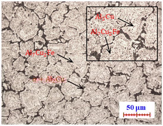
Figure 1.
The microstructure of 2219 Al alloy.
2.2. Experiment
Usually, the solidus temperature of 2219 aluminum alloy is 816 K, and the service temperature is usually below 573 K. The actual forming strain rate of 2219 aluminum alloy ranges from 0.01 s−1 to 10 s−1. It was been determined that the temperature range for the compression experiments would be between 573 K and 773 K. Additionally, the strain rate for these experiments was determined to be between 0.01 s−1 and 10 s−1. The homogenized metal was used to machine hot compression specimens with a diameter of 10 mm and a height of 15 mm. As shown in Table 2, 25 samples were heated to temperatures of 573 K, 623 K, 673 K, and 773 K at a rate of 5 K/s and were subsequently subjected to isothermal compression at deformation rates of 0.01 s−1, 0.1 s−1, 1 s−1, and 10 s−1, with deformation amounts of 60% each. After compression, the specimens were quenched immediately in a water medium to preserve their high-temperature deformation microstructure. A tantalum foil with a thickness of 0.1 mm was placed between the specimen and the tool to minimize friction during hot deformation. The flow stress–strain curves were automatically recorded from load-stroke data during the isothermal compression experiments with Gleeble 3500 (Gleeble, Poestenkill, NY, USA).
Table 2.
Isothermal compression test parameters.
Figure 2 shows the true stress–strain curves obtained under different deformation conditions. During the initial compression deformation, work hardening dominates, leading to a rapid increase in flow stress. The presence of generating dislocations in a material impedes the movement of other dislocations, increasing the material’s resistance to deformation. Generating dislocations arise when the lattice planes of the material are distorted due to plastic deformation, creating a type of imperfection in the crystal structure. These dislocations act as obstacles to the movement of other dislocations, slowing down the deformation process. As the strain increases, dynamic softening starts to play a more significant role. Dynamic softening occurs due to a variety of mechanisms, including dynamic recovery, recrystallization, and grain refinement, among others. These mechanisms can partially or completely reverse the work hardening that has occurred in the material, leading to a reduction in flow stress. The point at which work hardening and dynamic softening balance out is referred to as peak stress. It can be observed from the figure that the flow stress increased as the temperature decreased and the strain rate increased. This is because a lower temperature and a higher strain rate increase the amount of work hardening and generating dislocations, respectively, which in turn increases the material’s resistance to deformation. Conversely, a higher temperature and a lower strain rate promote dynamic softening, leading to a reduction in flow stress.
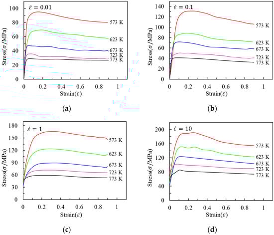
Figure 2.
Flow stress–strain curves of 2219 Al alloy during hot compression at strain rates of (a) 0.01 s−1, (b) 0.1 s−1, (c) 1 s−1, and (d) 10 s−1.
The observed phenomenon can be attributed to several factors. First, the temperature increase weakens the bond between metal atoms, which in turn reduces the thermal activation energy required for dislocations and boundaries to move. This results in the material becoming more susceptible to plastic deformation [20]. Second, an increase in the strain rate leads to a more rapid deformation process, resulting in a higher density of dislocations within the material. This increased density of dislocations is responsible for the observed increase in flow stress. Finally, the shorter time available for accumulating activation energy results in reduced recovery behavior, which contributes to the consumption of dislocations. These factors collectively lead to an increase in flow stress under the specified deformation conditions.
To facilitate the determination of material parameters for the constitutive model, the flow stress curves were discretized into 10 equidistant intervals. This was done to ensure that sufficient data were available for accurately fitting the constitutive model. The intervals spanned from a strain of 0.04 to 0.8 to capture the complete range of plastic deformation experienced by the material during the isothermal compression experiments. The stress values presented in Table 3 were derived via linear interpolation, grounded in the flow curves depicted in Figure 2.
Table 3.
Stress data obtained at different strain levels (the units of the strain rate, temperature, and stress are s−1, K, and MPa, respectively).
3. Constitutive Model
3.1. Arrhenius Model
3.1.1. Basic Expression
The Arrhenius (AH) constitutive model is widely used to predict flow stress, due to its simple form, few parameters, and good generalized ability. The AH model was first proposed by Sellars and McTegart [21]. The formula for the model is shown in Equation (1), which relates the flow stress (σ) to the temperature (T), strain rate (), and material parameters (A, α, n, and β).
where A, α, n, and β are material parameters, Q is the activation energy (J·mol−1), R is the universal gas constant (8.314 J·K−1·mol−1), T is the absolute temperature (K), is the strain rate (s−1), and σ is the flow stress (MPa). To simplify the calculation of material parameters for the Arrhenius model, Equation (1) can be transformed into Equation (2) by taking logarithms on both sides of the equation.
3.1.2. Parameter Solution
The material parameters of ln, , , and at each strain level can be obtained with multivariate nonlinear regression of Equation (2) using flow stress data (Table 3). Next, the curves of -, -, - and - can be obtained using these regression data. The polynomial fitting of -, -, - and - is conducted to obtain the constitutive equation with strain compensation by using flow data listed in Table 3.
As shown in Figure 3, a fifth-degree polynomial was used to fit these data, and expressions for each parameter were obtained. The degree of polynomial can be determined according to the regression accuracy, but using too high a degree can lead to overfitting. The Arrhenius constitutive equation for 2219 Al alloy can be obtained by introducing the value from Table 4 into Equation (1).
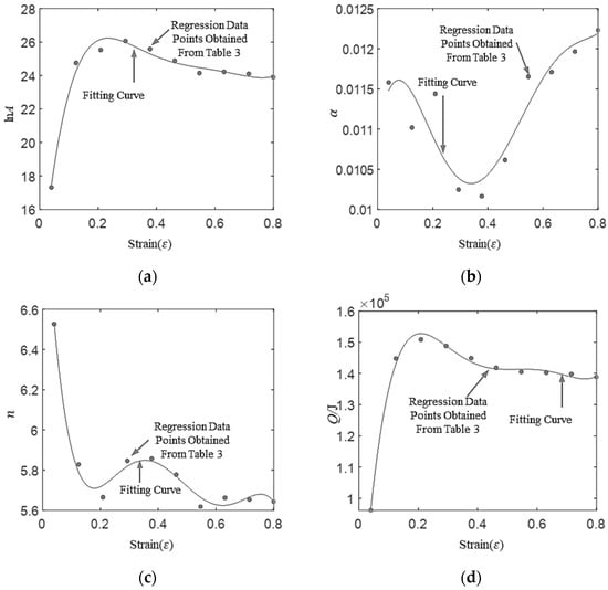
Figure 3.
Regression values of material parameters at different strain levels and their polynomial fitting curves: (a) lnA-ε, (b) α-ε, (c) n-ε, and (d) Q-ε.
Table 4.
Polynomial regression coefficients of material parameters for the Arrhenius constitutive model.
3.2. New Constitutive Model
3.2.1. Higher-Order Derivatives
It is well known that when the strain is constant, the key to building a constitutive model of 2219 Al alloy is to establish a functional relationship between stress, the strain rate, and temperature. The Arrhenius model is an implicit function that is complicated in practical application. For easy application, the relationship between stress, the strain rate, and temperature can be defined as an explicit function, which can be expressed as . According to the Taylor series, the function of can be approximated with a polynomial. To study the relationship between logarithmic stress, the logarithmic strain rate, and temperature, the partial derivatives of logarithmic stress with respect to temperature and logarithmic strain rate can be calculated with numerical calculations. The discrete formulas of derivatives include the forward difference, backward difference, and central difference. To maintain the number of rows and columns of the stress data (shown in Table 3), forward and backward differences are used at the start and end boundaries, respectively, and the central difference is used in the middle region. Next, the high-order partial derivatives of logarithmic stress with respect to the temperature and logarithmic strain rate for the stress data can be calculated using Equations (3)–(5).
where is the order of the partial derivative and and are indices of the strain rate and temperature, respectively. For instance, when = 1 and = 1, represents the logarithmic stress with a strain rate of 0.01 s−1 and a temperature of 573 K. The maximum values of and are the numbers of strain rates and temperatures, respectively. When = 1 or = 1, Equation (3) should be replaced by Equation (4), which is a backward difference.
When = 5 or = 5, Equation (3) should be replaced by Equation (5), which is a forward difference.
The logarithmic stress–temperature and logarithmic stress–logarithmic strain rate curves are shown in Figure 4.
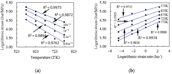
Figure 4.
Curves at a strain of 0.209: (a) logarithmic stress and temperature and (b) logarithmic stress and logarithmic strain rate.
As can be seen from Figure 4a,b, the minimum value of the square of the correction between logarithmic stress and temperature was 0.9762, which is significantly larger than 0.8, and the minimum value of the square of the correction between logarithmic stress and logarithmic strain rate was 0.9715, which is also significantly larger than 0.8. Therefore, there is a strong linear relationship between logarithmic stress and temperature, as well as between logarithmic stress and the logarithmic strain rate.
To further analyze the higher-order relationship between logarithmic stress and temperature, the higher-order partial derivatives of logarithmic stress with respect to temperature were calculated using Equations (3)–(5). As can been seen from Figure 5a,b, the maximum absolute value of the first-order derivative at a strain of 0.209 was close to 0.008 for all strain rate and temperature levels. Meantime, as shown in Figure 5c,d, the maximum absolute value of the second-order derivative was significantly less than that of the first-order derivative and the maximum absolute value of the second-order derivative at a strain of 0.209 was close to 0 for all strain rate and temperature levels. If fact, these phenomena exist at other strain levels. Therefore, to build a high-precision constitution model, the first-order derivative must be considered for the constitutive model and the second-order derivative is assumed as 0. Therefore, a first-order approximation between logarithmic stress and temperature should be considered to construct a high-precision constitutive model without significantly increasing material parameters.
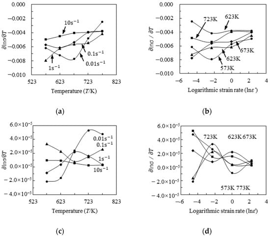
Figure 5.
At a strain of 0.209, the higher-order partial derivatives of logarithmic stress with respect to temperature at different temperatures (573 K, 623 K, 673 K, 723 K, and 773 K) and strain rates (0.01 s−1, 0.1 s−1, 1 s−1, and 10 s−1): (a) first-order derivative distributed on temperature, (b) first-order derivative distributed on the logarithmic strain rate, (c) second-order derivative distributed on temperature, and (d) second-order derivative distributed on the logarithmic strain rate.
Similarly, to further analyze the higher-order relationship between logarithmic stress and the logarithmic strain rate, the high-order partial derivatives of logarithmic stress with respect to the logarithmic strain rate were calculated using Equations (3)–(5).
As can be seen from Figure 6a,b, the maximum absolute value of the first-order partial derivatives of logarithmic stress with respect to the logarithmic strain rate at a strain of 0.209 were close to 0.2 for all strain rate and temperature levels. As can be seen from Figure 6c,d, the maximum absolute value of the second-order partial derivatives of logarithmic stress with respect to the logarithmic strain rate at a strain of 0.209 were close to 0.02 for all strain rate and temperature levels. As can be seen from Figure 6e,f, the maximum absolute value of the third-order partial derivatives of logarithmic stress with respect to the logarithmic strain rate at a strain of 0.209 were close to 0.005 for all strain rate and temperature levels. As can be seen from Figure 6g,h, the msaximum absolute value of the fourth-order partial derivatives of logarithmic stress with respect to the logarithmic strain rate at a strain of 0.209 were close to 0.0009 for all strain rate and temperature levels. Obviously, the third- and fourth-order partial derivatives were significantly less than the first-order derivatives. The difference between the maximum and minimum values of the third-order partial derivatives was equal to 0.0088. In fact, these phenomena exist at other strain levels. Next, to reduce the material parameters without significantly reducing the prediction accuracy of the new model, the third-order partial derivative was assumed as a constant at all strain rates and temperatures and the fourth-order partial derivative was assumed as 0 at all strain rates and temperatures. Therefore, a third-order approximation between logarithmic stress and the logarithmic strain rate should be considered to construct a high-precision constitutive model without significantly increasing material parameters.
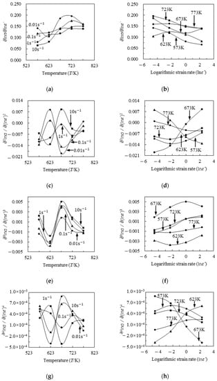
Figure 6.
At a strain of 0.209, the higher-order partial derivatives of logarithmic stress with respect to the logarithmic strain rate at different temperatures (573 K, 623 K, 673 K, 723 K, and 773 K) and strain rates (0.01 s−1, 0.1 s−1, 1 s−1, and 10 s−1): (a) first-order derivative distributed on temperature, (b) first-order derivative distributed on the logarithmic strain rate, (c) second-order derivative distributed on temperature, (d) second-order derivative distributed on the logarithmic strain rate, (e) third-order derivative distributed on temperature, (f) third-order derivative distributed on the logarithmic strain rate, (g) fourth-order derivative distributed on temperature, and (h) fourth-order derivative distributed on the logarithmic strain rate.
3.2.2. Expression for the New Model
The conclusion extracted from the previous section is that to construct a high-precision constitutive model without significantly increasing material parameters, a first-order approximation between logarithmic stress and temperature and a third-order approximation between logarithmic stress and the logarithmic strain rate should be considered. Therefore, the expression of the new constitutive model is assumed in Equation (6).
where , , , , and are material parameters. To easily obtain the material parameters, the general form of the new model is shown in Equation (7).
where ~ are material parameters, which can be obtained using multiple linear regression.
where n is the number of strain interpolations, which is equal to 10 in this study. and are temperatures and strain rates corresponding to the strain interpolation, respectively. is the parameter column vector, which is equal to , and is the error column vector with a size of 1 × n.
3.2.3. Parameter Solution
The material parameters can be obtained easily using multilinear regression (Equation (8)) based on the interpolation data provided in Table 3. The fifth-degree polynomial was used to fit these material parameters, and the expression of each parameter was obtained. The degree of polynomial can be determined according to the regression accuracy, but too high a degree leads to overfitting. The new constitutive equation of 2219 Al alloy can be obtained by introducing Table 5 into Equation (6).
Table 5.
Polynomial regression coefficients of material parameters for the new constitutive model.
The formulas for the material parameters are listed in Table 5, and the corresponding curves are shown in Figure 7. Although the number of material parameters was more than that of the Arrhenius model, the solution for these material parameters was simpler. The new model only used multiple linear regression to solve the parameters, while the Arrhenius model requires multiple nonlinear regression. It is often difficult to find global optimal parameters for multiple nonlinear regression, but it is easy for multiple linear regression. Therefore, the new model is better than the Arrhenius model for solving material parameters.
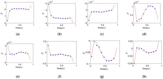
Figure 7.
Regression values of material parameters at different strain levels and their polynomial fitting curves: (a) -ε, (b) -ε, (c) -ε, (d) -ε, (e) -ε, (f) -ε, (g) -ε, (h) -ε.
3.3. Prediction Accuracy Comparison
To analyze prediction accuracy, the predicted data of both the Arrhenius model and the new model are shown in Figure 8. The solid lines in Figure 8 represent experimental flow stress curves, the red circles represent prediction values of the Arrhenius model, and the blue • symbols represent prediction values of the new model.
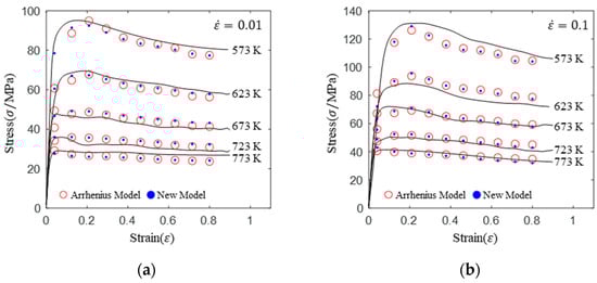
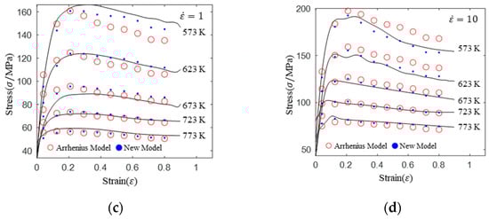
Figure 8.
Comparison of prediction flow stress and experimental flow stress for the Arrhenius and new models: (a) 0.01 s−1, (b) 0.1 s−1, (c) 1 s−1, and (d) 10 s−1.
As can be seen from Figure 8a,b, at a low strain rate (0.01 s−1 and 0.1 s−1,) the prediction accuracy of the new model was slightly higher than that of the Arrhenius model. The comparison of correlation coefficients in Figure 9a,b can prove this phenomenon. However, as shown in Figure 8c,d, the prediction accuracy of the new model was significantly higher than that of the Arrhenius model at high strain rate (1 s−1 and 10 s−1) and low temperature (573 K and 623 K) levels. In addition, with increasing deformation temperature, the prediction accuracy of the Arrhenius model also increased at a constant strain rate. The new model had a similar prediction accuracy at each deformation temperature and deformation strain rate, and the prediction accuracy was higher than that of the Arrhenius model.
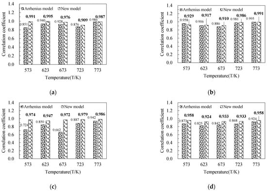
Figure 9.
Comparison of the correlation coefficients between predicted stress and experimental stress at different strain rates for the Arrhenius and new models: (a) 0.01 s−1, (b) 0.1 s−1, (c) 1 s−1, and (d) 10 s−1.
To further analyze the prediction accuracy, correlation coefficients were calculated at different strain rates and temperatures and are shown in Figure 9. It is well known that a larger value of the correlation coefficient indicates a higher prediction accuracy. As can be seen from Figure 9a,b, all the other correlation coefficients of the new model were slightly higher than those of the Arrhenius model, with one particular exception (0.1 s−1 and 573 K). In addition, the correlation coefficient of the Arrhenius model was slightly higher than that of the new model in this particular exception. As can be seen from Figure 9c,d, all the correlation coefficients of the new model were significantly higher than those of the Arrhenius model.
4. Hot Processing Maps and Microstructure
4.1. Hot Processing Maps
Based on the analysis conducted in the previous section, it was found that the new constitutive model exhibits a significant level of precision in predicting flow stress. Therefore, the establishment of hot processing maps for 2219 aluminum alloy was carried out using the new constitutive model. According to Prasad’s theory [22], the hot deformation of a material is a process of power dissipation, and the total energy applied on the workpiece is divided into two parts, namely (1) power dissipated for plastic deformation (G) and (2) power dissipated for microstructural transformation (J). So, the total power (P) can be expressed as:
The ratio between G and J was determined using the strain rate sensitivity and can be calculated as:
In nonlinear energy dissipation, the energy dissipation rate () can be introduced to characterize the proportion of energy consumed by organizational evolution. The greater the energy dissipation rate, the greater the energy consumption of organizational evolution, and the greater the change in organizational morphology.
According to Narayan’s study [22], when the rate of entropy generation in the system does not match the rate of applied entropy, the system experiences flow instability. Its criterion is as follows:
where is the instability factor. The analytical formula of the strain rate sensitivity can be derived using the new constitutive model (Equation (7)):
Next, the analytical formulas of the energy dissipation rate and the instability factor can be obtained by putting Formula (13) into Formulas (11) and (12). Hot processing maps at low (0.2), medium (0.6), and high (0.9) strain levels were drawn, as shown in Figure 10.
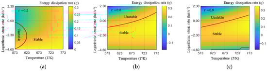
Figure 10.
Hot processing maps at various strain levels: (a) 0.2, (b) 0.6, and (c) 0.9.
In Figure 10, the depth of color on the surface represents the magnitude of the energy dissipation rate and the red solid line represents the boundary between the stable and unstable regions. As can be seen from Figure 10a–c, with an increase in temperature, the energy dissipation increased at a constant strain rate. With an increase in the strain rate, the energy dissipation first increased and then decreased at constant temperature. The stable region was located within a medium strain rate range. Considering that the deformation of metals is a continuous process, the best region for hot processing is in the temperature range of 673–773 K and the strain rate range of 0.1–1 s−1. When the strain rate is 0.01 s−1, the energy dissipation rate is low and the energy consumed by microstructural evolution is relatively small, which may result in coarse grains.
4.2. Microstructure
To further study the hot processing maps, the microstructures of each compression specimen are listed in Table 6. At the same temperature, the microstructure sizes (Table 6b,c,f,g,i,j,m,n,q,r) at strain rates of 0.1 s−1 and 1 s−1 were smaller than those under other strain rate conditions. This is consistent with the conclusion of the heat treatment diagram, that is, when the strain rate is 0.1 s−1 or 1 s−1, the energy dissipation rate is the highest. It can be seen from the hot processing diagram (Figure 10c) that when the temperature was 573 K and the strain rate was 10 s−1, the energy dissipation rate was lower and the degree of recrystallization was smaller. Therefore, under these conditions, the microstructure of the material is the coarsest, which was proved by the microstructure of the specimen (shown in Table 6d). When the strain rate was 0.01 s−1 (shown in Table 6a,e,h,l,p), the size of the microstructure was large, which is indicated by the hot processing maps (Figure 10c). In addition, when the temperature was constant (e.g., Table 6a–d), the grain size first decreased and then increased with an increase in the strain rate, which verifies the correctness of the hot processing maps. In summary, the results of microstructure analysis are in good agreement with the prediction results of the hot working diagram. Hot processing maps can be used to guide the hot working process formulation of 2219 aluminum alloy.
Table 6.
Microstructures under different experimental conditions.
5. Discussion
This article discussed the results of isothermal compression experiments and microstructure analysis experiments performed at different temperatures and strain rates. A new constitutive model was proposed, which is based on the partial derivatives of the experimental flow data, without requiring significant increases in material parameters. The study compared and analyzed the predictive accuracy of the new model and the classic Arrhenius model. The main conclusions are as follows:
- (1)
- The flow stress level increases significantly with increasing strain rate and decreasing deformation temperature. Since 2219 aluminum alloy is a strain-rate- and temperature-sensitive material, its constitutive relationship must take into account the influence of the temperature and strain rate. A first-order approximation between logarithmic stress and temperature and a third-order approximation between logarithmic stress and the logarithmic strain rate should be considered to construct a high-precision constitutive model without significantly increasing material parameters.
- (2)
- The prediction accuracy of the new model is slightly higher than that of the Arrhenius model at low strain rate levels (0.01 s−1 and 0.1 s−1). The new model displays a significantly higher prediction accuracy than the Arrhenius model at high strain rate (1 s−1 and 10 s−1) and low temperature (573 K and 623 K) levels. In addition, with increasing deformation temperature, the prediction accuracy of the Arrhenius model also increases at a constant strain rate. The new model has a similar prediction accuracy at each deformation temperature and deformation strain rate, and its prediction accuracy is higher than that of the Arrhenius model.
- (3)
- With an increase in temperature, the energy dissipation increases at a constant strain rate. With the increase of the strain rate, the energy dissipation first increases and then decreases at a constant temperature. The best region for hot processing is in the temperature range of 673~773 K and the strain rate range of 0.1~1 s−1. The results of microstructure analysis are in good agreement with the prediction results of hot processing maps. Hot processing maps can be used to guide the hot working process formulation of 2219 aluminum alloy.
In addition, the prediction accuracy of the new model established in this article is extremely high within the experimental temperature, strain rate, and strain range. However, the prediction accuracy cannot be guaranteed in areas outside the experimental range. Therefore, when using this model in numerical simulation, it is necessary to verify whether the simulation parameter range is within the experimental range. The method of constructing a new model in this article is a universal method, so it can be further studied on other materials.
Author Contributions
J.W. put forward the relevant algorithms and ideas, wrote the article, and carried out the experiments. G.X. developed the calculation programs. J.Z. guided the writing process. All authors have read and agreed to the published version of the manuscript.
Funding
This research was funded by the National Natural Science Fund (grant no. Joint Fund U2030120) and the Chongqing Board of Education, China (scientific research project grant no. KJQN202000813).
Data Availability Statement
All data generated or analyzed during this study are included in this published article.
Acknowledgments
Thanks to all the authors for their contributions to this article.
Conflicts of Interest
The authors declare no conflict of interest.
References
- Prabhu, T.R. Effects of ageing time on the mechanical and conductivity properties for various round bar diameters of AA 2219 Al alloy. Eng. Sci. Technol. Int. J. 2017, 20, 133–142. [Google Scholar] [CrossRef]
- He, H.; Yi, Y.; Huang, S.; Zhang, Y. An improved process for grain refinement of large 2219 Al alloy rings and its influence on mechanical properties. J. Mater. Sci. Technol. 2019, 35, 55–63. [Google Scholar] [CrossRef]
- Zhang, L.; Li, X.; Li, R.; Jiang, R.; Zhang, L. Effects of high-intensity ultrasound on the microstructures and mechanical properties of ultra-large 2219 Al alloy ingot. Mater. Sci. Eng. A 2019, 763, 138154. [Google Scholar] [CrossRef]
- Kaibyshev, R.; Sitdikov, O.; Mazurina, I.; Lesuer, D.R. Deformation behavior of a 2219 Al alloy. Mater. Sci. Eng. A 2002, 334, 104–113. [Google Scholar] [CrossRef]
- Sellars, C.M.; McTegart, W.J. On the mechanism of hot deformation. Acta Metall. 1966, 14, 1136–1138. [Google Scholar] [CrossRef]
- Johnson, G.R.; Cook, W.H. A constitutive model and data for metals subjected to large strains, high strain rates and high temperatures. Eng. Fract. Mech. 1983, 21, 541–548. [Google Scholar]
- Senthilkumar, V.; Balaji, A.; Arulkirubakaran, D. Application of constitutive and neural network models for prediction of high temperature flow behavior of Al/Mg based nanocomposite. Trans. Nonferrous Met. Soc. China 2013, 23, 1737–1750. [Google Scholar] [CrossRef]
- Lin, Y.C.; Chen, X.M. A critical review of experimental results and constitutive descriptions for metals and alloys in hot working. Mater. Des. 2011, 32, 1733–1759. [Google Scholar] [CrossRef]
- Liu, L.; Wu, Y.; Gong, H.; Wang, K. Modification of constitutive model and evolution of activation energy on 2219 aluminum alloy during warm deformation process. Trans. Nonferrous Met. Soc. China 2019, 29, 448–459. [Google Scholar] [CrossRef]
- Jia, X.; Wang, Y.; Zhou, Y.; Cao, M. The study on forming property at high temperature and processing map of 2219 Aluminum alloy. Metals 2021, 11, 77. [Google Scholar] [CrossRef]
- Wang, H.; Qin, G.; Li, C. A modified Arrhenius constitutive model of 2219-O aluminum alloy based on hot compression with simulation verification. J. Mater. Res. Technol. 2022, 19, 3302–3320. [Google Scholar] [CrossRef]
- He, H.; Yi, Y.; Cui, J.; Huang, S. Hot deformation characteristics and processing parameter optimization of 2219 Al alloy using constitutive equation and processing map. Vacuum 2019, 160, 293–323. [Google Scholar] [CrossRef]
- LI, S.; Chen, W.; Krishna, S.B.; Dong, W.J.; Chen, X. Flow Behavior of AA5005 Alloy at High Temperature and Low Strain Rate Based on Arrhenius-Type Equation and Back Propagation Artificial Neural Network (BP-ANN) Model. Materials 2022, 15, 3788. [Google Scholar] [CrossRef] [PubMed]
- Shayanpoor, A.A.; Rezaei Ashtiani, H.R. The phenomenological and physical constitutive analysis of hot fow behavior of Al/Cu bimetal composite. Appl. Phys. A 2022, 128, 636. [Google Scholar] [CrossRef]
- Jiang, D.; Zhang, J.; Liu, T.; Li, W.; Wan, Z.; Han, T.; Che, C.; Cheng, L. A modified Johnson–Cook model and microstructure evolution of as-extruded AA 2055 alloy during isothermal compression. Metals 2022, 12, 1787. [Google Scholar] [CrossRef]
- Xiao, Y.; He, Z. A Continuum Constitutive Model for a 7003-Aluminum Alloy Considering the Stress State and Strain Rate Effects. Iran. J. Sci. Technol. Trans. Mech. Eng. 2022, 128, 1–11. [Google Scholar] [CrossRef]
- Zhang, P.; Chen, M. Progress in characterization methods for thermoplastic deforming constitutive models of Al–Li alloys: A review. J. Mater. Sci. 2020, 55, 9828–9847. [Google Scholar] [CrossRef]
- Shin, H.; Ju, Y.; Choi, M.K.; Ha, D.H. Flow Stress Description Characteristics of Some Constitutive Models at Wide Strain Rates and Temperatures. Technologies 2022, 10, 52. [Google Scholar] [CrossRef]
- Guo, Y.; Zhang, J.; Zhao, H. Microstructure evolution and mechanical responses of Al–Zn–Mg–Cu alloys during hot deformation process. J. Mater. Sci. 2021, 56, 13429–13478. [Google Scholar] [CrossRef]
- Zhou, Y.; Lin, X.; Wang, Z.; Tan, H.; Huang, W. Hot deformation induced microstructural evolution in local-heterogeneous wire plus arc additive manufactured 2219 Al alloy. J. Alloys Compd. 2021, 865, 158949. [Google Scholar] [CrossRef]
- Richardson, G.J.; Sellars, C.M.; Tegart, W. Recrystallization during creep of nickel. Acta Metall. 1996, 14, 1225–1236. [Google Scholar] [CrossRef]
- Narayana Murty, S.V.S.; Nageswara Rao, B.; Kashyap, B.P. Identification of flow instabilities in the processing maps of AISI 304 stainless steel. J. Mater. Process. Technol. 2005, 166, 268–278. [Google Scholar] [CrossRef]


Disclaimer/Publisher’s Note: The statements, opinions and data contained in all publications are solely those of the individual author(s) and contributor(s) and not of MDPI and/or the editor(s). MDPI and/or the editor(s) disclaim responsibility for any injury to people or property resulting from any ideas, methods, instructions or products referred to in the content. |
© 2023 by the authors. Licensee MDPI, Basel, Switzerland. This article is an open access article distributed under the terms and conditions of the Creative Commons Attribution (CC BY) license (https://creativecommons.org/licenses/by/4.0/).