Article

Glycine Dissolution Behavior under Forced Convection

Chair of Process Systems Engineering, Technical University of Munich, 85354 Freising, Germany
*
Author to whom correspondence should be addressed.
Crystals 2023, 13(2), 315; https://doi.org/10.3390/cryst13020315
Submission received: 30 January 2023 / Revised: 9 February 2023 / Accepted: 10 February 2023 / Published: 14 February 2023

Abstract

:
The integration of a flow-through cell into a Mach–Zehnder interferometer offers the possibility to study the dissolution of crystals in detail. The influence of flow on the displacement velocity of a specific crystal facet and the distribution of the solute concentration around the crystal are measured simultaneously in a time-resolved manner. The disintegration from the crystal surface and the mass transfer into the solvent can be separated. We aim to establish an in vitro experiment that improves the quality of prediction for the bioavailability of active pharmaceutical ingredients. In the presented feasibility study, glycine was used as a model substance. It was successfully demonstrated that the set-up is suitable for observing disintegration and mass transfer separately. The description of the dissolution rate in terms of the Sherwood number as a function of Reynolds, Schmidt and Grashof numbers clearly shows that with increasing flow rate there is a transition from natural to forced convection as the dominant mass transfer mechanism. Temporal and spatial resolved concentration fields visualize the convective mass transfer and also show the influence of convection on the diffusive boundary layer. No limitation of the dissolution by surface disintegration could be found in the examined range of flow rates.

1. Introduction

Drug discovery and drug product development are cost-intensive processes that take up to 10 years, going through various testing phases [1]. Estimations of research and development costs for a new drug amount to USD 2.826 billion. Clinical tests account for approximately 50–58% of this sum [2]. For time and cost reasons, ineffective drug development should therefore be excluded at an early stage, at the latest before the start of the clinical phase. The bioavailability of active pharmaceutical ingredients (API) is a crucial factor. Particularly in the case of orally administered drugs, low solubility or the slow dissolution of the crystalline form of the API hinders absorption in the human body. Nevertheless, it is estimated that about 90% of the global market share of pharmaceutical formulations are orally administered drugs [3]. For several decades, research therefore aimed to increase solubility. Suggested approaches are, e.g., the synthesis of salt- or co-crystal forms or the addition of excipients [3,4]. An in vitro study of the solubility and especially the dissolution kinetics achieved with these methods is essential before entering the clinical phase.
The United States Pharmacopeia (USP) recommends seven different apparatuses for routine, in vitro dissolution tests [5]. Most of the studies published on dissolution kinetics used USP Apparatus 2, the paddle apparatus [6,7,8,9]. Some also used USP Apparatus 4, the flow-through cell apparatus [10,11,12]. The advantage of the latter is the well-defined flow and that the API does not accumulate in the solvent that comes into contact with the sample. Within all these methods, the dissolution kinetics are determined by the time-dependent concentration of the drug in the solvent. Uddin et al. [5] write that such in vitro dissolution studies provide the closest link to in vivo performance. We hypothesize that a resilient prediction of the dissolution in the human body requires that face-specific API disintegration rates and mass transfer mechanisms are studied separately. For example, for aspirin [13], paracetamol [14] or ibuprofen [14], dissolution is assumed to be diffusion-limited. The hydrodynamic conditions then have a great influence on the dissolution kinetics, since the diffusion limitation is overcome at higher flow rates [15,16]. Furthermore, the validation of methods for the in silico prediction of resolution rates of APIs as suggested by Elts et al. [17] or Dogan et al. [18] also requires experiments in which a distinction between surface disintegration and mass transfer is possible. A number of methods have already been presented for determining face-specific dissolution or growth rates in a flow-through cell. Offiler et al. [19] determined the face-specific growth rate of α -glycine crystals in an optical cell by automated image analysis that includes automatic indexing of the facets by Hough transform. Shekunov et al. [20] studied the growth and dissolution of selected facets of paracetamol in a Michelson interferometer. Moazami Goudarzi et al. [21] integrated the flow-through cell in an X-ray tomography setup to monitor the 3D structure during dissolution. Østergaard et al. [22] observed the dissolution of different APIs with UV imaging. In addition to the projection of the crystal, they obtained spatially and temporally resolved 2D concentration fields. The multi-microscope approach of Adobes Vidal et al. [23] combines atomic force microscopy, scanning ion conductance microscopy and optical microscopy and therefore allows the study of face-specific dissolution rates, surface quality and the surrounding concentration field.
Another promising approach to simultaneously measure facet-specific growth or dissolution rates and the surrounding concentration field is interferometric methods. In the reviews by Verma and Shlichta [24], Srivastava et al. [25] or Eder and Briesen [26], numerous studies are presented in which the concentration field in the vicinity of a crystal is measured using interferometric methods. Some authors furthermore determined the growth or dissolution rate from a sequence of interferograms [27,28,29,30]. Adawi et al. [31] and Hou et al. [32] visualized gravity-induced natural convection and described its influence on crystal growth. However, until now there have been few studies in which measurements are carried out under forced convection [33,34].
We propose a measurement method in which an optical flow-through cell is integrated into a Mach–Zehnder interferometer. We describe a procedure where both the 2D concentration field and the face-specific dissolution rate can be determined from the interferograms. α-glycine is investigated as a model substance. Depending on the flow velocity, we investigate the face-specific dissolution rate of the (110)-surface of the crystal and the width of the diffusive layer at the phase boundary. By visualizing the concentration field and considering dimensionless numbers, the dominating mechanism for mass transfer during dissolution can be identified.

2. Materials and Methods

2.1. Experimental Set-Up

In the next two sections, the main focus is on the description of the measurement procedure. Further detailed information, especially on the components used, can be found in Appendix A.

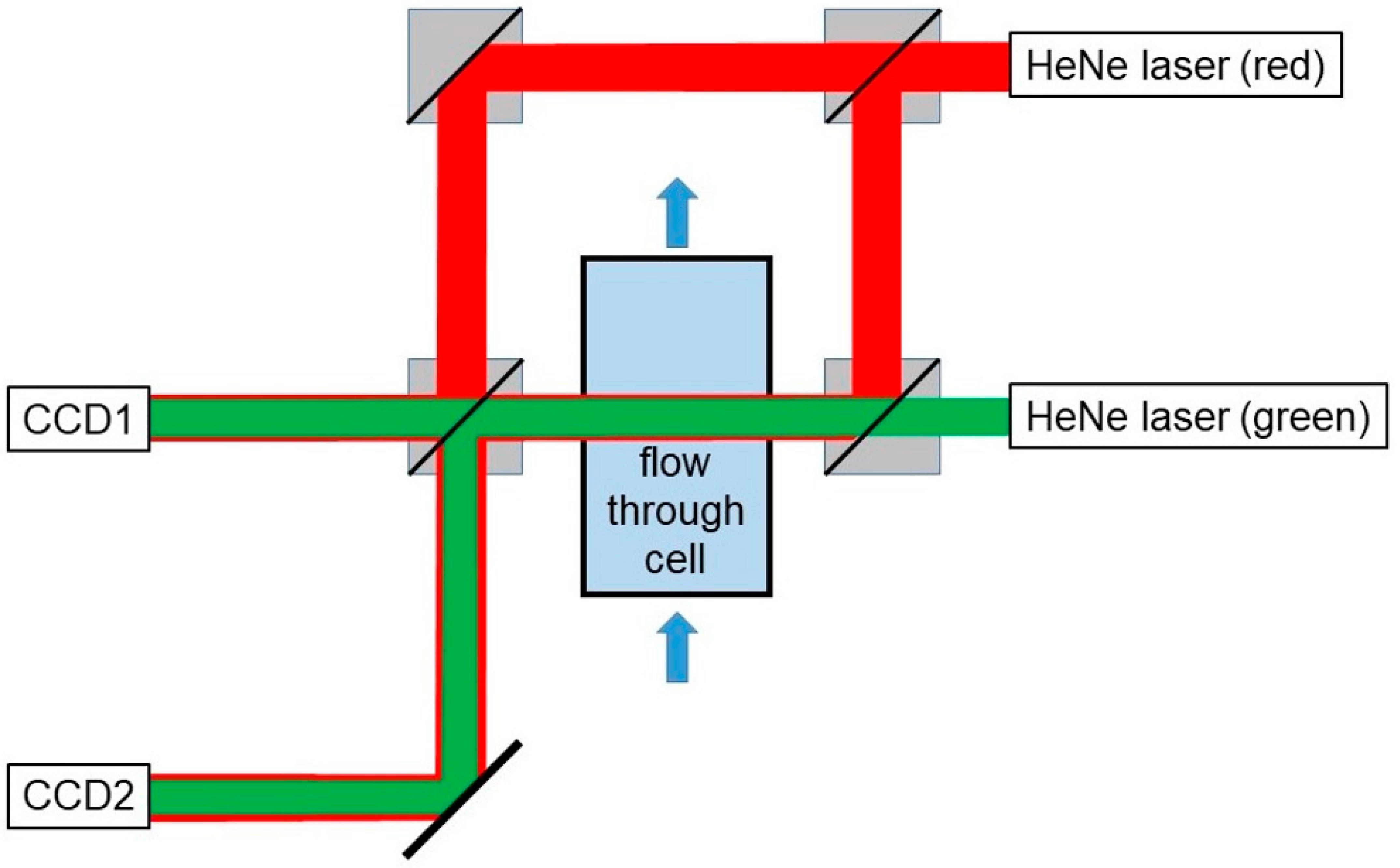
2.1.1. Optical Set-Up

We use an optical measurement technique to simultaneously observe the shape of a dissolving crystal and the concentration field in its environment. The concentration field in the vicinity of the crystal is observed with a Mach–Zehnder interferometer (see Figure 1). A red HeNe laser with expanded beam is used as light source. The test beam of the interferometer crosses the flow-through cell with the mounted crystal. When the test beam and the reference beam, which is not influenced by the sample, are superimposed, an interference pattern is created. Each interference fringe represents a constant phase shift between the test and reference beams. Since the concentration along the test beam affects the phase shift, the 2D concentration field can be determined from the interferogram. The pattern is observed with two color CCD cameras, CCD1 with a field of view of 12.1 × 7.6 mm2 and a resolution of 6.29 µm/px and CCD2 with a smaller field of view (4.5 × 3.7 mm2) but higher resolution (1.83 µm/px). By tilting the beamsplitters, the distance and the direction of the interference fringes can be adjusted. The fringes in the bulk solution should be perpendicular to the crystal surface, have a distance that allows sufficient local resolution, but be clearly separated.
According to the set-ups described by Van Dam and Mischgofsky [35] and Eder et al. [30], the expanded beam of a green HeNe-laser is aligned parallel to the test beam of the Mach–Zehnder interferometer. When the cameras are focused on the crystal, their green channels provide sharp images of the crystal without superimposed interference fringes, whereas the red channels show the interference pattern. During the experiments, images were recorded every 10 s with both cameras.

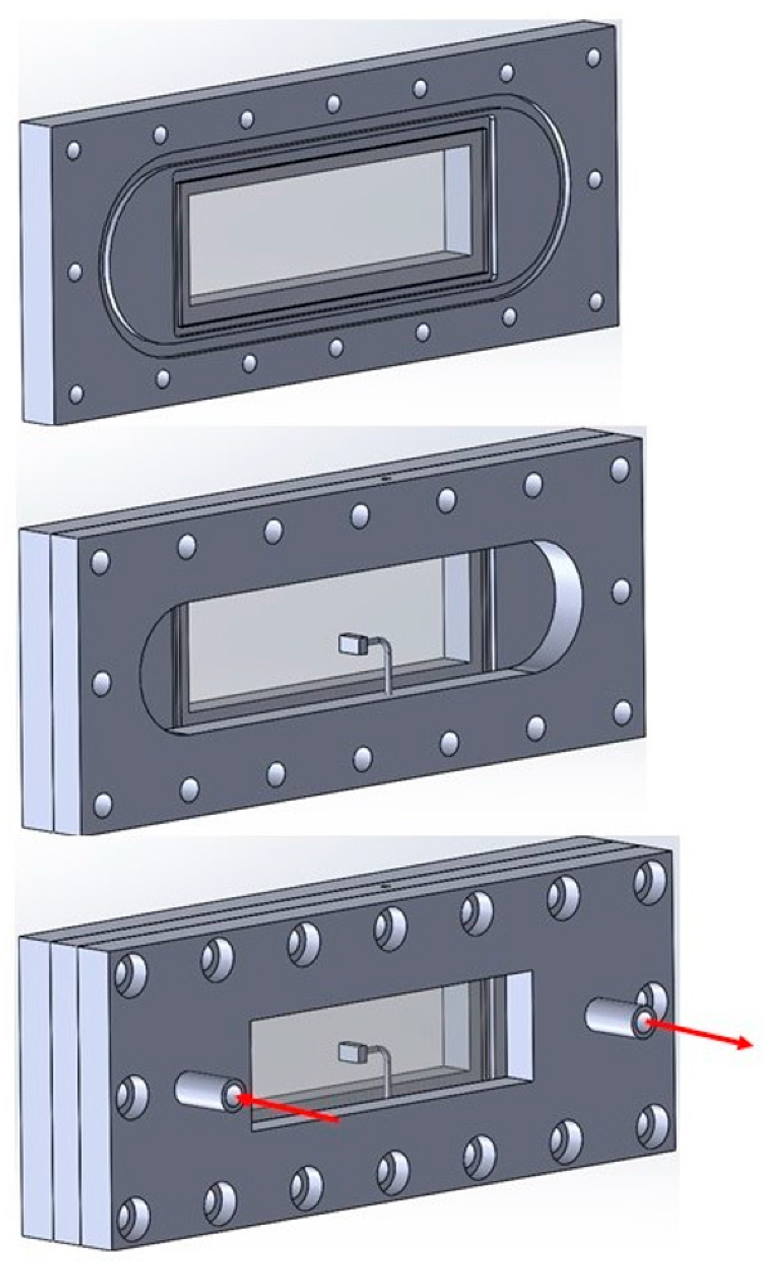
2.1.2. Fluidmechanical Set-Up

The flow-through cell (see Figure 2) consists of three aluminum plates sealed against each other by O-rings. Glass windows in the outer plates allow optical access for the interferometric measurement. The optically freely accessible area is 70 × 22 mm2. Tube connections are integrated in one of these plates as inlet and outlet connections for the flow (red arrows in Figure 2). The middle plate defines the channel geometry. The channel length was 110 mm. A height of 24 mm was chosen to be able to observe the convection around the crystal. The plate thickness and thus the channel width should be adapted to the crystal size in order to keep concentration gradients along the observation direction low. In the experiments presented here, a plate with 5 mm thickness was used.
We studied flow rates from stagnant solvent up to 800 mL/min. We used two different pumps to achieve different magnitudes of flow rates. For flow rates up to 17.5 mL/min, a Syrris Atlas syringe pump was used. Higher flow rates were achieved with the gear pump Verdergear VGS040. Using this setup, a mean flow velocity in the flow-through cell of up to 111 mm/s can be set. For the series of measurements described in Section 3.2 and Section 3.4, at least twelve different velocities were set for each of the three investigated solute concentrations.
In all experiments, we circulated 300 mL of solvent. In order to keep the temperature constant, the inlet to the flow-through cell was passed through a water bath with a temperature that was kept constant at 25 °C. To improve heat exchange, the solvent flows through an aluminum block acting as heat exchanger with contact areas of 40 cm2 to the solvent and 200 cm2 to the liquid in the water bath. Outside the heat exchanger and the flow-through cell, silicone tubing was used. The temperature at the outlet of the cell was kept in the range 25.0 ± 0.5 °C.

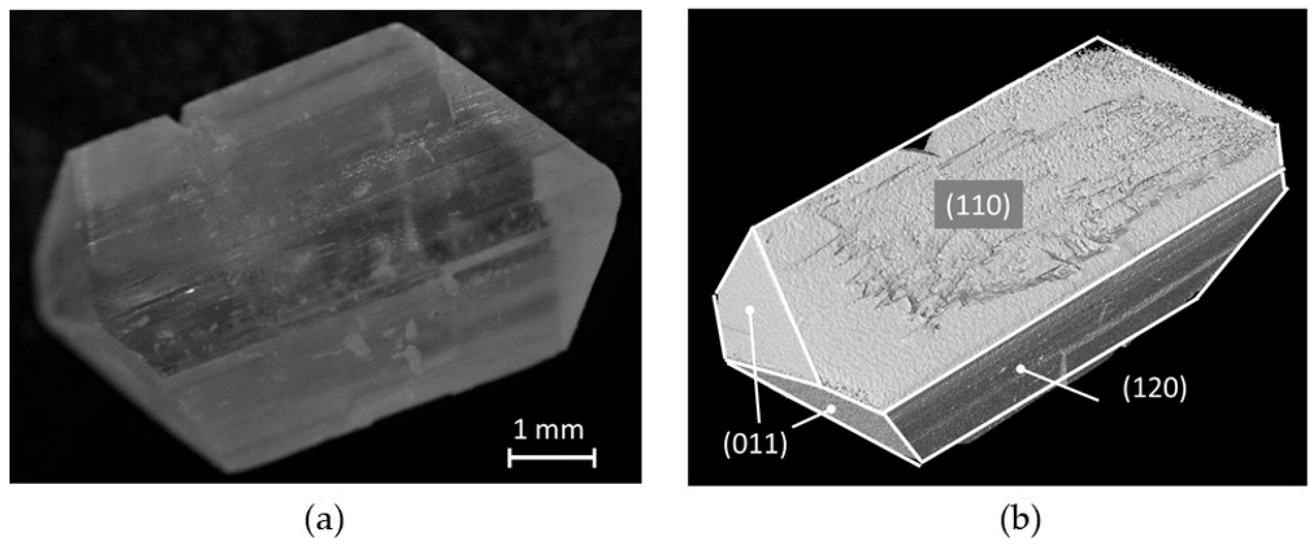
2.2. Crystals and Solvents

We used α-glycine crystals and aqueous glycine solutions as a model system because the required material data are available in the literature. Glycine crystals were grown at 25 °C in crystallization dishes sealed with parafilm. A saturated solution of 0.25 g of glycine (Apollo Scientific Ltd., Whitefield Rd, Bredbury, Stockport, Cheshire, SK6 2QR, UK. Catalogue No: BIG0709 CAS Number: 56-40-6 MDL Number: MFCD00008131 Purity: >99%) per 1 g of demineralized water was seeded with a few sub-mm crystals from a previous experiment. In the following, glycine concentrations will be reported as loads, i.e., g glycine/g water. The habit of the crystals is similar to the α-glycine crystals shown by Han et al. [36]. Based on the data provided by Marsh for the unit cell of α-glycine [37], we identified the crystal facets from three-dimensional computer tomography (µ-CT) data with the method developed by Kovacevic et al. [38]. As shown in Figure 3, the facet (110) is dominating. The crystals were harvested when the (110) face reached the desired size of about 3.5 mm in width.
The crystal is mounted with one (110) facet on a wire crystal carrier. The UV-initiated cyanoacrylate glue UHU Booster (UHU GmbH & Co. KG, Herrmannstr. 7, 77815 Bühl/Baden, Germany) was used for this purpose. The crystal is positioned in the center of the channel of the flow cell shown in Figure 2. It is aligned so that the opposite (110) facet will be perpendicular to the flow. Two intersecting (011) surfaces point upwards and downwards, respectively.
Aqueous glycine solutions of different concentrations (0.11, 0.16 and 0.21 g/g in experiments with forced convection) were used as solvents during the dissolution experiments. Due to the differing saturations of the solvents, the model system glycine-water can be used to check whether the method is suitable for different concentration differences between bulk and crystal surface. This is a property that is necessary for transferability to other substances. The increase in the glycine concentration during the experiments, which is caused by the recirculation of the solvent, amounts to a maximum of 0.0002 g/g when the crystal is completely dissolved and is neglected.

2.3. Image Analysis

The interferometer yields series of images that show the crystals during different states of their dissolution and the corresponding interference patterns. We use MATLAB 2022 routines with classical image-processing methods to extract the displacement of the crystal outline and the 2D concentration fields. In the following sections, we explain the basic procedure for the image processing. A detailed list of the MATLAB commands used and the parameters set can be found in Appendix B.

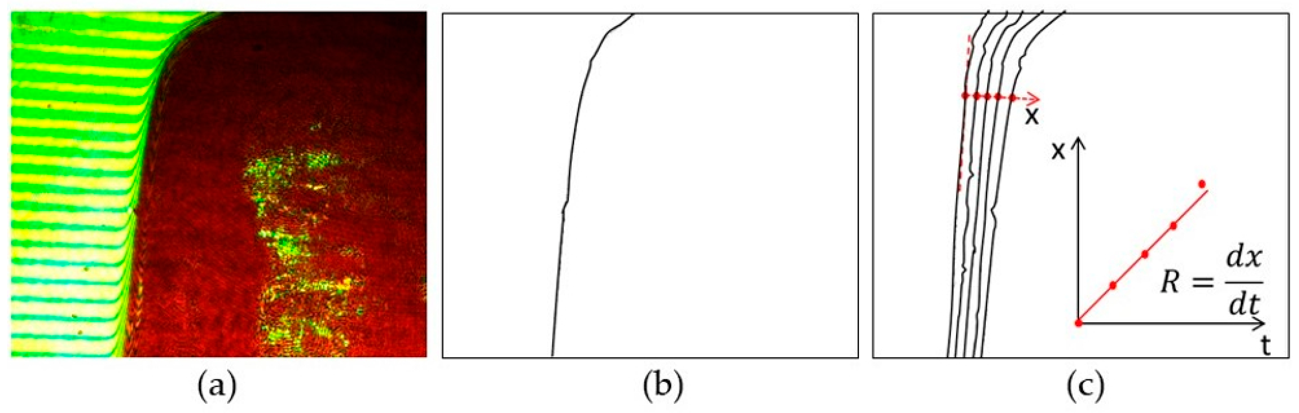
2.3.1. Extraction of Crystal Outline and Face Displacement Velocity

Figure 4 shows the determination of the face displacement velocity, starting with the original image (Figure 4a). The green channel of the images shows a sharp image of the crystal that is not influenced by interference fringes. Therefore, it is used to extract the crystal outline. After a slight smoothing, the image is binarized. Further image processing removes small dropouts and artifacts outside of the crystal and smoothes the silhouette of the crystal. Subsequently, the crystal outline is created (Figure 4b). Each image of the series yields one outline. Based on the outlines, face displacement velocities are extracted. A normal vector to the (110) facet in the first image (red arrow Figure 4c) is created. The position of the (110) facet along this vector is then determined for all following outlines and plotted against time. The increased rounding towards the end of the test leads to a deviation from linearity. The gradient from the linear initial phase was therefore used as the face displacement velocity R .

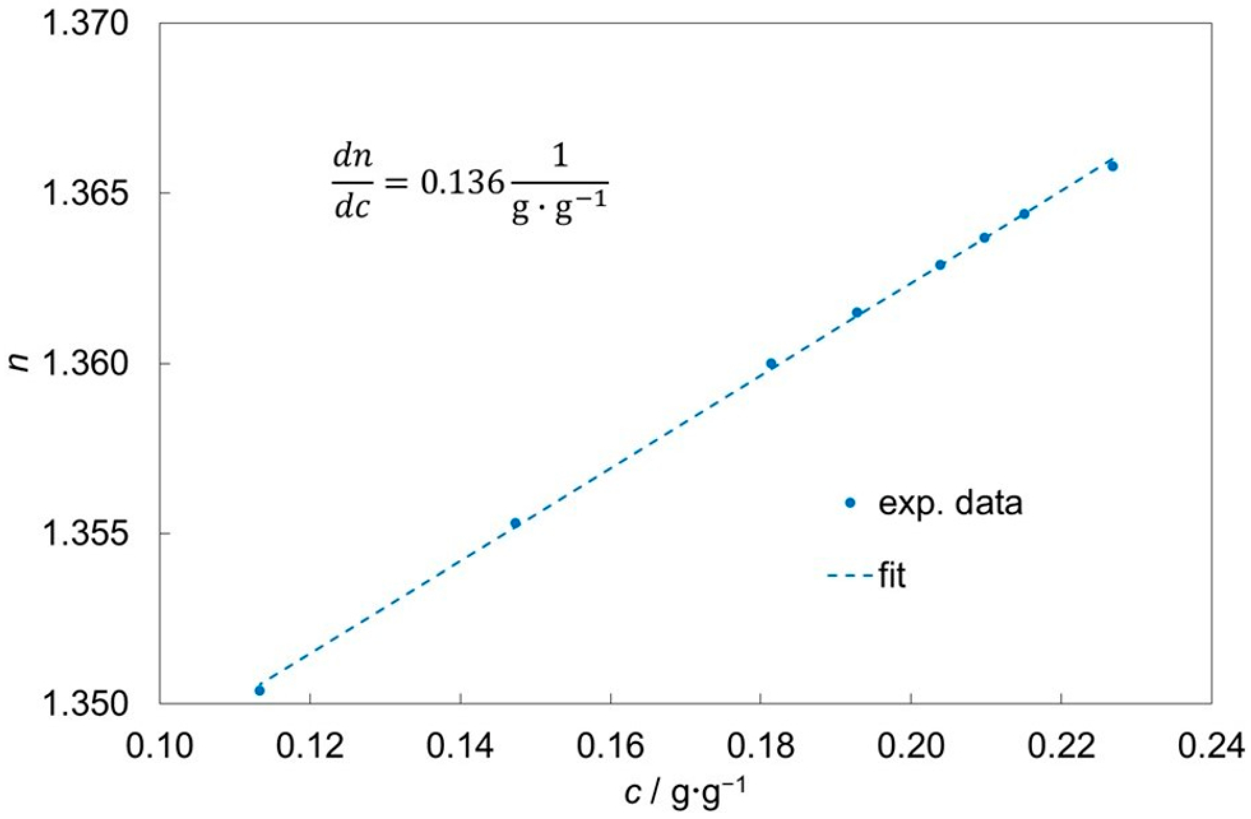
2.3.2. Extraction of the Concentration Field

The recorded series of interferograms not only show the shape of the crystal, but the glycine concentration in the liquid phase can be derived from the course of the interference fringes. These are only visible in the red channel. The procedure for the calculation of the concentration field and the thickness of the diffusive boundary layer is illustrated in Figure 5.
Starting with the original image (Figure 5a), the red channel is smoothed and binarized. For further image processing, the area of the crystal is masked. The remaining interference fringes are then shrinked to lines. At this stage of the evaluation, the thickness of the diffusive layer x D is measured. Generally, x D is defined by the Nernst–Brunner equation, [39] or [40] (p. 225)
1 A   ·   d m d t = D   ·   c c S x D
with solute mass m , diffusion coefficient D , crystal surface A , bulk concentration c and saturation concentration c S . The concentrations are given in kg/m3. Combining Equation (1) with Fick’s first law, it seems obvious to measure the extent of the diffusion zone by the intersection of the tangents to the fringes at the phase boundary and in the bulk. However, the tangent at the crystal surface cannot be determined with sufficient accuracy. Therefore we use the method proposed by Onuma et al. [41]. The distance between the crystal surface and the point where the interference fringes begin to bend is defined as the thickness of the diffusive layer x D (Figure 5b).
In the following, lines belonging to one interference fringe are connected. The interference fringes are sorted in ascending order and numbered. The assigned number indicates the local phase shift Φ x , y between reference and test beam as a multiple of 2 π . Interpolation leads to the phase shift in the entire unmasked area. This phase shift field must be compared with the one that would arise in the case of homogeneous concentration, i.e., without the crystal. In order to calculate this hypothetical field Φ 0 x , y , a region unaffected by the crystal is selected and the phase shift field is extrapolated to the rest of the unmarked area. The difference in phase shift produced by dissolving the crystal corresponds to a difference in the mean refractive index
Δ n x , y = λ 2 π   ·   Φ x , y Φ 0 x , y s ,
with the thickness of the flow cell s   = 5 mm and the wavelength λ = 632.8 nm of the red HeNe laser. The change in concentration (Figure 5c) is calculated by dividing Δ n by the concentration contrast factor
n c = 0.136 1 g / g .
It was determined in the concentration range 0.10–0.22 g/g by measuring the refractive index at 25° C with the Krüss DR6200-T (Krüss GmbH, Borsteler Chaussee 85, 22453 Hamburg, Germany) laboratory refractometer (see Figure 6).

3. Results and Discussion

3.1. Face Displacement Velocity in Stagnant Solvents

We started with dissolution experiments in stagnant glycine solutions with varying glycine concentration. Figure 7 shows the measured face displacement velocities R 0 . The data are correlated using a least-square regression by
R 0 c = 130   µ m min   ·   1 c c s 1.46 .
c s = 0.25 g/g is the solubility of α-glycine in water at 25 °C [42].
According to Mullin [40] (pp. 227–228) and Bermingham [43] (pp. 16–17), dissolution processes are usually expected to have a linear dependence of dissolution rate on undersaturation, which is characteristic for diffusion-controlled processes. The higher exponent of 1.46 can possibly be explained by the fact that a surface disintegration step influences the dissolution kinetics, as it is, e.g., reported by Bovington and Jones [44]. Another explanation could be that mass transfer from crystal surface to solution is not entirely driven by diffusion, but also by gravity-induced natural convection, originated by the higher density of the solution at the crystal surface compared to the bulk solution. The influence of natural convection on crystal growth was investigated, e.g., by Adawi et al. [31] and Hou et al. [32].
Figure 7. Face displacement velocities of the (110) glycine facet in stagnant aqueous glycine solutions.
Crystals 13 00315 g007

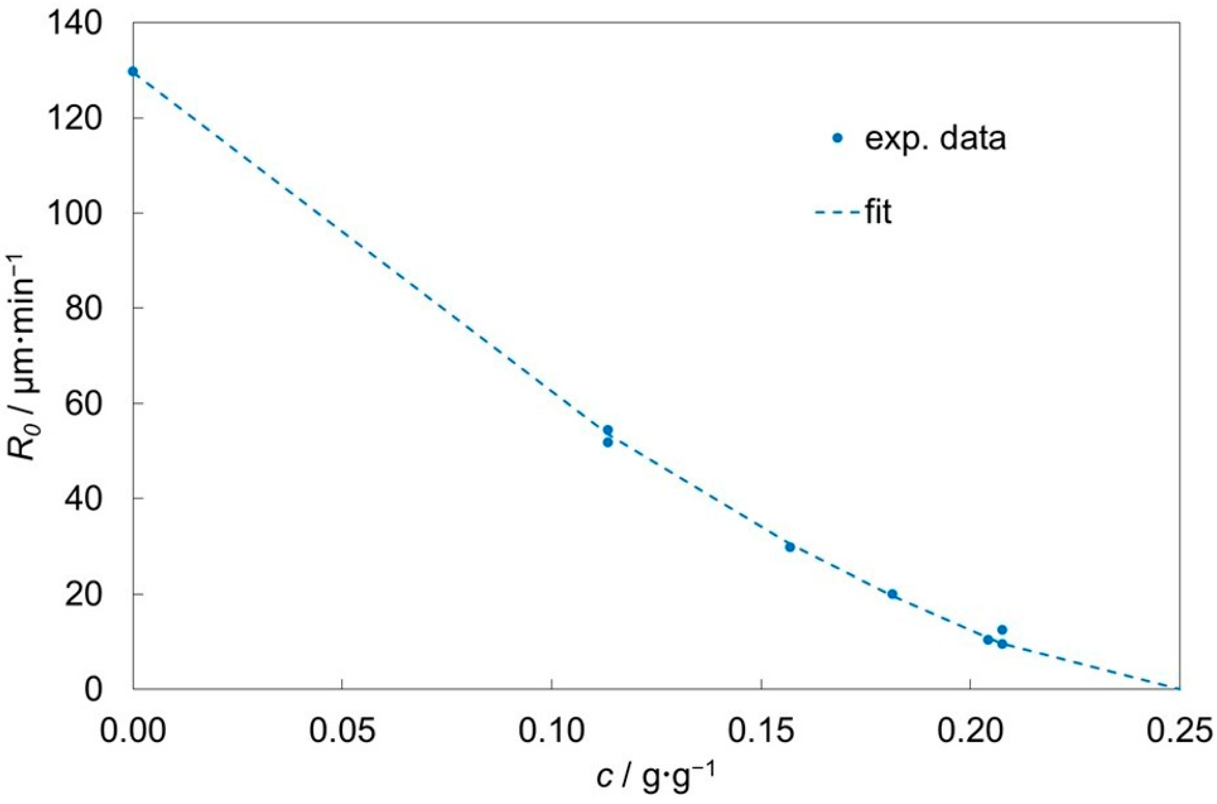
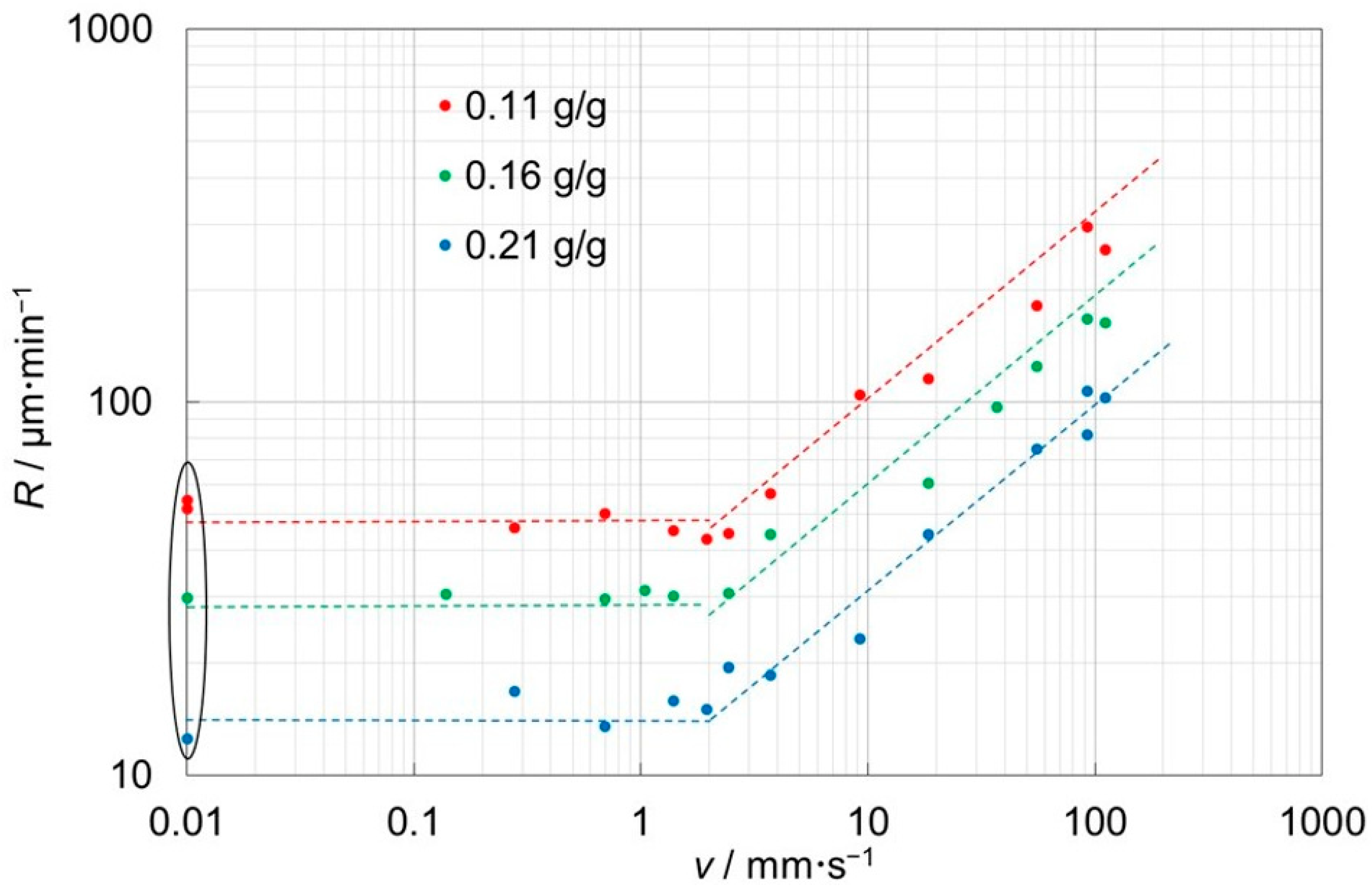
3.2. Face Displacement Velocities under Forced Convection

To investigate the influence of the flow rate on the crystal dissolution, experiments at a constant flow rate were performed. The use of crystals of similar shape and size ensures the comparability of the measured face displacement velocities, because the flow conditions in the vicinity of the crystal depend on the size and habit of the crystal. Dissolution was observed until the crystal was rounded to the point where the target facet could no longer be identified. To illustrate the change of crystal shape, Figure 8 shows a crystal (a) before filling the cell, (b) at the start of the experiment and (c) when the experiment was terminated. A new crystal was used for each sample point in Figure 9.
In the range of achievable flow rates, the face displacement velocity was determined for concentrations 0.11, 0.16 and 0.21 g/g (saturation 44, 64, 84%). The results are shown in Figure 9. Two areas can be seen. Lines are drawn for better orientation. Up to the kink point v K   2 mm/s, the face displacement velocity R is constant; above v K it seems to increase with the square root of the velocity. Both the kink point and the velocity dependence are very similar for the three investigated concentrations. The face displacement velocity for higher flow velocities can thus be estimated with the equation
R c , v = R 0 c   ·   v v K .
The increase in the face displacement velocity for v > v K indicates a change in mass transfer regime.

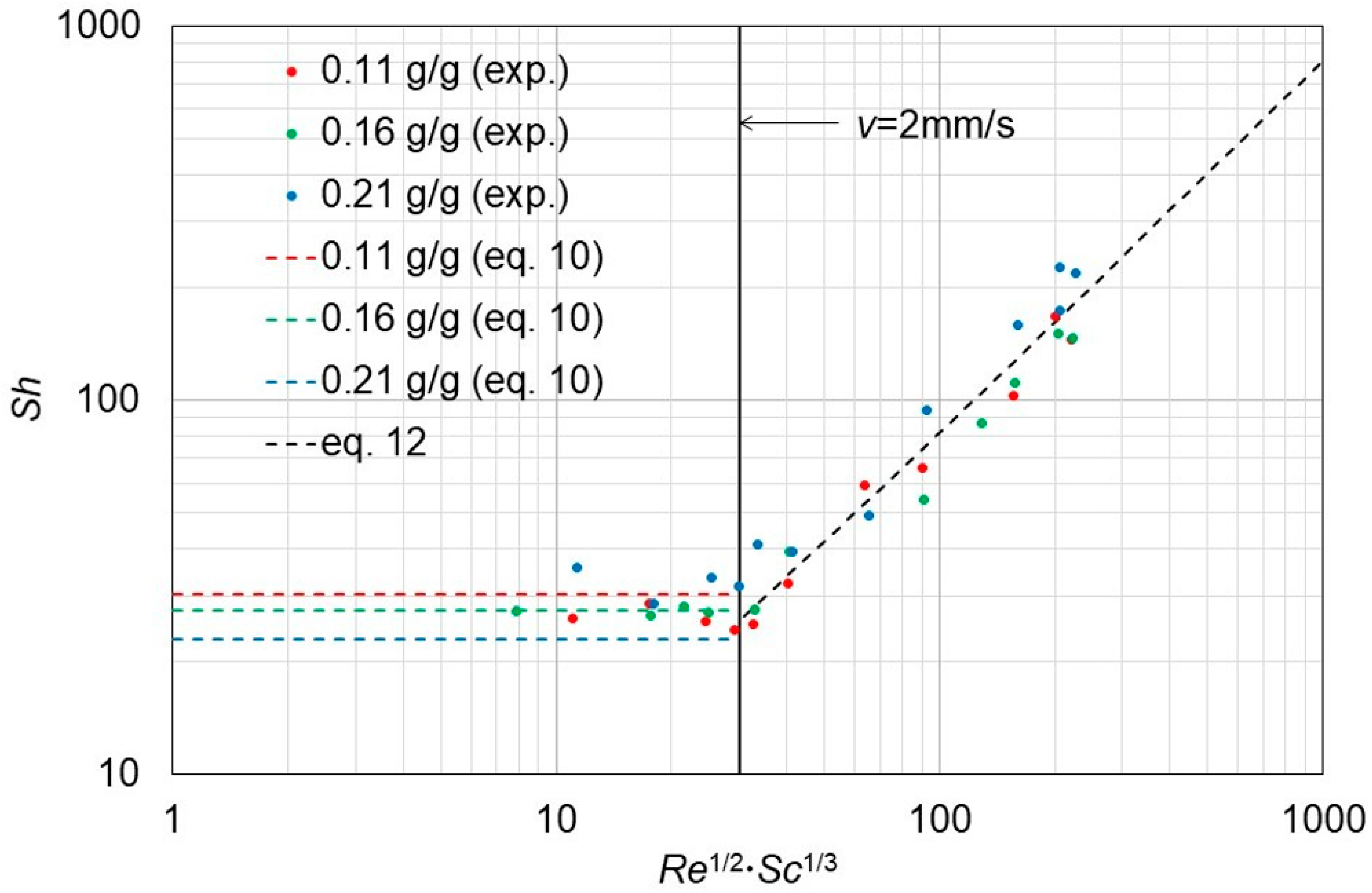
3.3. Description in Terms of Dimensionless Numbers

The observed trends of the dissolution rates indicate that mass transfer by forced convection becomes dominant when the flow velocity increases. Following, e.g., Mullin and Garside [45], Bomio et al. [46] or Pohar and Likozar [47], the dependence of the Sherwood number ( S h ) on the Grashof number ( G r ), particle Reynolds number ( R e ) and Schmidt ( S c ) number was investigated to identify the predominant transport mechanism. The characteristic dimensionless numbers are calculated based on experimental data for the face displacement velocity R , the mean flow velocity v and the glycine concentration c .
S h = L D   ·   R c S c
G r = g   ·   L 3   ·   ρ   ·   ρ S ρ η 2
R e = ρ   ·   v   ·   L η
S c = η ρ   ·   D
To determine the average characteristic length L , ten crystals of typical form and size were weighed. The diameter of an equivalent sphere with the average crystal volume is L = 4.1 mm. The material data required for the calculation of the dimensionless numbers were taken from the literature. The density of glycine solutions ρ as well as the density of the saturated solution ρ S at the crystal surface are given by Ninni and Meirelles [48], the dynamic viscosity η is calculated with the empirical coefficients obtained by Devine and Lowe [49] and the diffusion coefficients D are calculated based on studies of Ma et al. [50].
For the description of the mass transfer in a stagnant solvent, an equation of the form
S h = 2.0 + A   ·   ( G r   ·   S c ) 1 / 4
has been proposed [45,46]. The first summand 2.0 is the theoretical value for spherical particles and purely diffusive mass transfer in the stagnant solvent. The second summand describes the enhancement of mass transfer by natural convection. Based on the face displacement velocity in stagnant solvent (Equation (4)), Sherwood numbers were calculated for the three concentrations investigated. Fitting Equation (10) to these results gives A = 0.36. Similar values are reported in the literature. Mullin and Garside [45] found a value of 0.564 for the growth of aluminum potassium sulphate, Bomio et al. [46] gave 0.477 for the dissolution of hexamethylene tetramine. Since the Sherwood numbers exceed those of the purely diffusive mass transfer by one order of magnitude, it can be assumed that mass transfer in the stagnant solvent is dominated by natural convection.
The relation
S h = B + C   ·   R e a   ·   S c b .
was proposed for the description of the mass transfer under forced convection [46,47]. The increase in the growth rate with v at high flow velocities (see Section 3.2) suggests a dependence of the Sherwood number on R e at higher Reynolds numbers. In the presented experiments, the Schmidt number is almost constant. Therefore, the exponent b is not significant and consequently b = 1 / 3 is taken from the literature. This leaves B and C as free parameters, fitted by minimizing the root-mean-square error (RMSE); the following correlation is distinguished:
S h = 1.80 + 0.80   ·   R e 1 / 2   ·   S c 1 / 3
Since forced convection is expected to dominate for v 2   mm / s , only these results were used for the fit. Note that S h = 1.80 in Equation (12) does not represent the Sherwood number in stagnant solvent.
Figure 10 shows the Sherwood numbers for the experiments with forced convection. No significant influence of concentration was detected. As expected, the trend of the Sherwood numbers also changes in the region of v = 2 mm/s. For lower flow velocities, the Sherwood number is almost constant. Since the value is significantly above 2, the mass transfer there is not purely diffusive but mainly governed by natural convection [45,46]. In the region where Equation (12) applies, mass transfer is dominated by forced convection.
By equating the two right-hand summands in Equations (10) and (12), the velocity above which the mass transfer is dominated by forced convection can be estimated.
v k e s t 0.2   ·   g   ·   L   ·   ρ S ρ ρ   ·   ρ   ·   D η . 6
For the three investigated concentrations in the range from 0.11 to 0.21 g/g, we obtain estimated values v k e s t = 2.7 to 1.4 mm/s for the kink velocity. Therefore, the estimate is in good agreement with the kink velocity of 2 mm/s that was observed in Section 3.2. Furthermore, this estimation illustrates that for smaller crystals (2. factor) or poorly soluble solutes (3. factor) convective mass transfer will dominate already at lower velocities.
If the dissolution at high flow velocity is limited by the surface disintegration rate, it results in a constant Sherwood number at high R e 1 / 2   ·   S c 1 / 3 -values. Though Mullin and Garside [45] observed the limitation by the surface integration step in their crystal growth experiments, we could not find a corresponding effect in our own dissolution experiments. In contrast to crystal growth, the time-consuming orientation of the molecules to fit the crystal lattice is not necessary during dissolution [43]. We assume that the observation of the disintegration limitation requires even higher flow velocity, because our model substance glycine dissolves in water too fast.

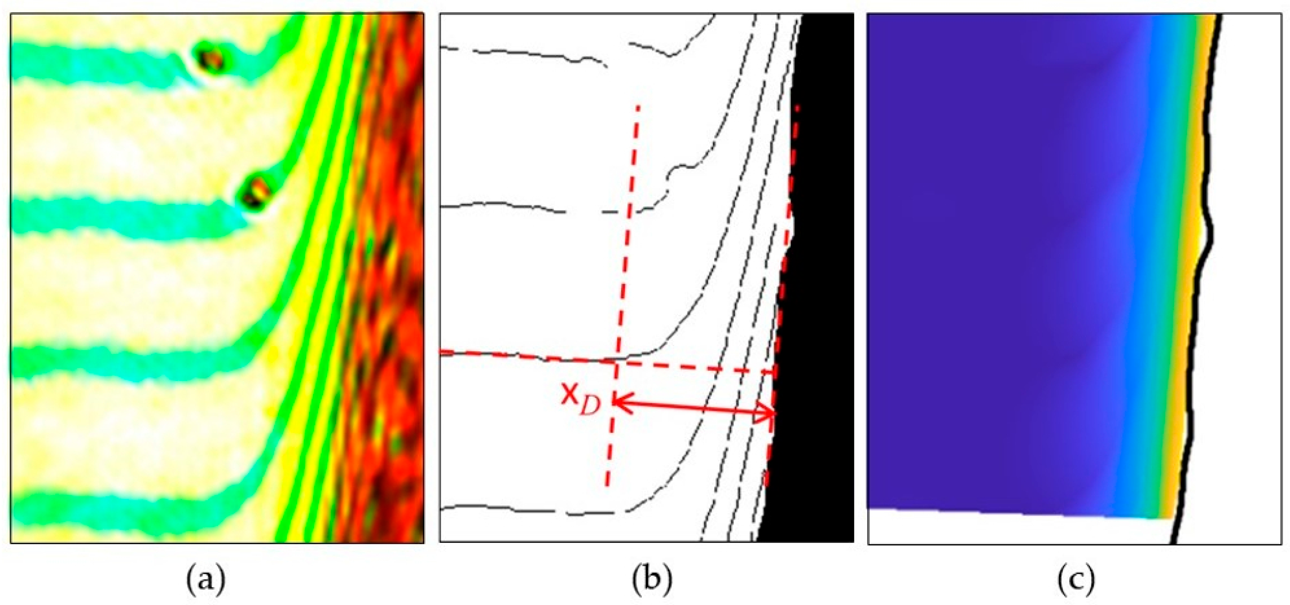
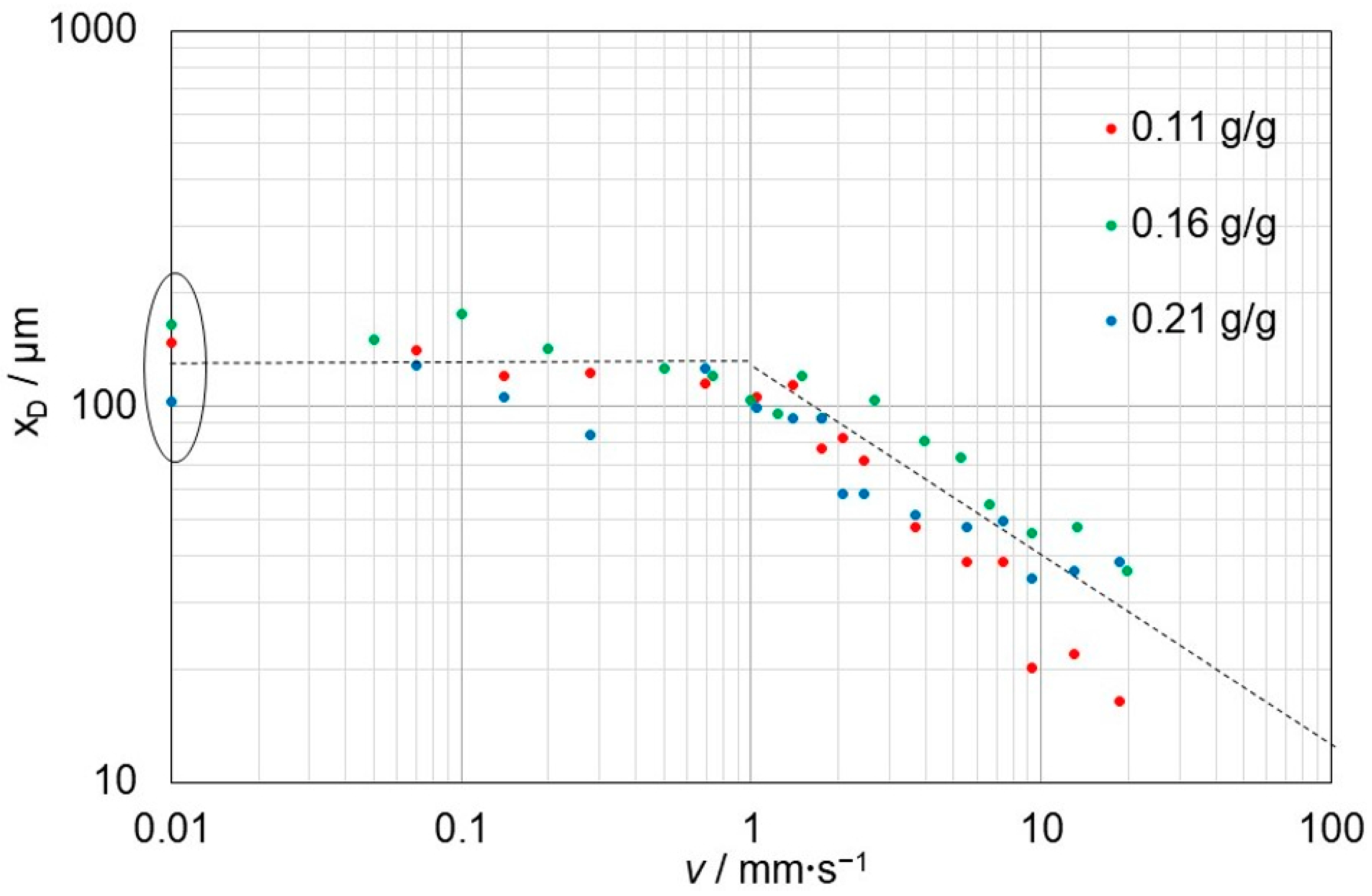
3.4. Thickness of the Diffusive Layer

The results described in Section 3.2 and Section 3.3 clearly show the influence of the convective mass transfer on dissolution. However, they do not allow any conclusions to be drawn about the diffusive boundary layer. Therefore, the thickness x D of the diffusive layer was determined in the interferograms recorded by CCD2. For each concentration, an experiment was performed in which the flow velocity was increased stepwise as soon as a stable diffusive layer was established. Because the crystal geometry changed only slightly during the course of this experiment, the influence of the crystal geometry on the flow was minimized.
The results are shown in Figure 11. Similar to the behavior of the face displacement velocity, the thickness of the diffusive layer is constant at low flow velocities. Using the face displacement velocity in stagnant solvent (Equation (3)), the Nernst–Brunner equation (Equation (1)) can be used to estimate the thickness of the diffusive boundary layer. Values of 90 (0.11 g/g) to 130 µm (0.21 g/g) are obtained. They are of the same magnitude as the values measured from the interferograms. However, the method used in this paper to determine the layer thickness (see Section 2.3.2) naturally yields larger values than the definition according to Nernst and Brunner. We conclude that the diffusive layer is reduced by natural convection. A significant concentration dependence of the layer thickness as could have been expected according to the estimates of the Nernst–Brunner equation was not observed. The diffusive layer is reduced as soon as the flow velocity exceeds approx. 1 mm/s. Below this velocity, the mean of the measured layer thickness is 125 µm ± 22 µm (standard deviation). Above, x D decreases approximately with 1 / v . Forced convection thus clearly reduces the diffusive layer thickness. In the experiments presented, the thickness of the diffusive layer is already reduced in the velocity range 1 to 2 mm/s, where the dissolution is found to be still dominated by natural convection.
Based on the course of the concentration towards the surface, it would be possible to determine the diffusive mass transfer based on Fick’s first law. However, in the presented experiments, the resolution of CCD2 was not sufficient to resolve the densely packed fringes close to the crystal–liquid interface. Assuming saturated solution at the crystal surface, the concentration difference across the diffusive boundary layer is then 0.04–0.14 g/g, depending on the bulk concentration. According to Equations (2) and (3), at least 26, max. 90 interference fringes are located almost parallel to the surface in the area of the diffusive layer. This problem will not arise with poorly soluble substances such as aspirin or paracetamol, or it can be reduced in future experiments by increasing the resolution of CCD2 at the expense of the field of view. Then, it will be possible to calculate the diffusive part of the mass transfer from the concentration gradient.

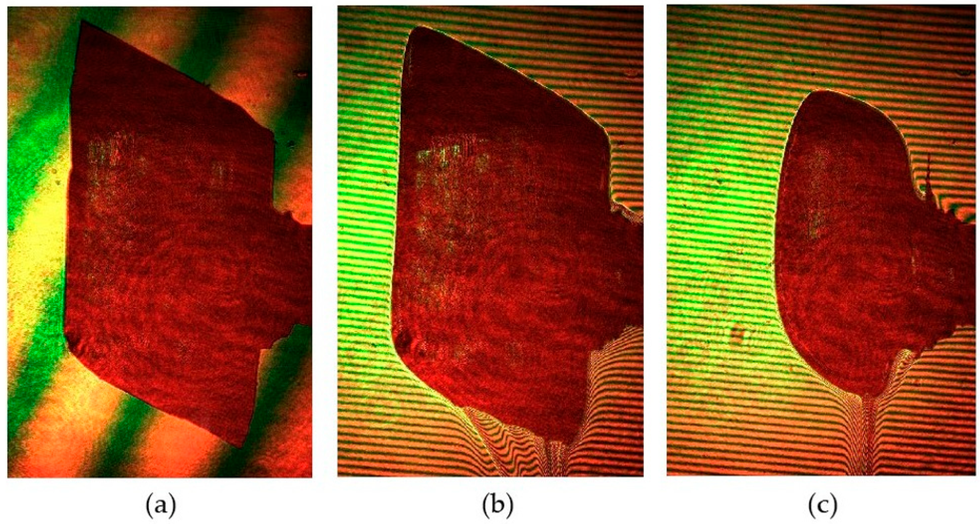
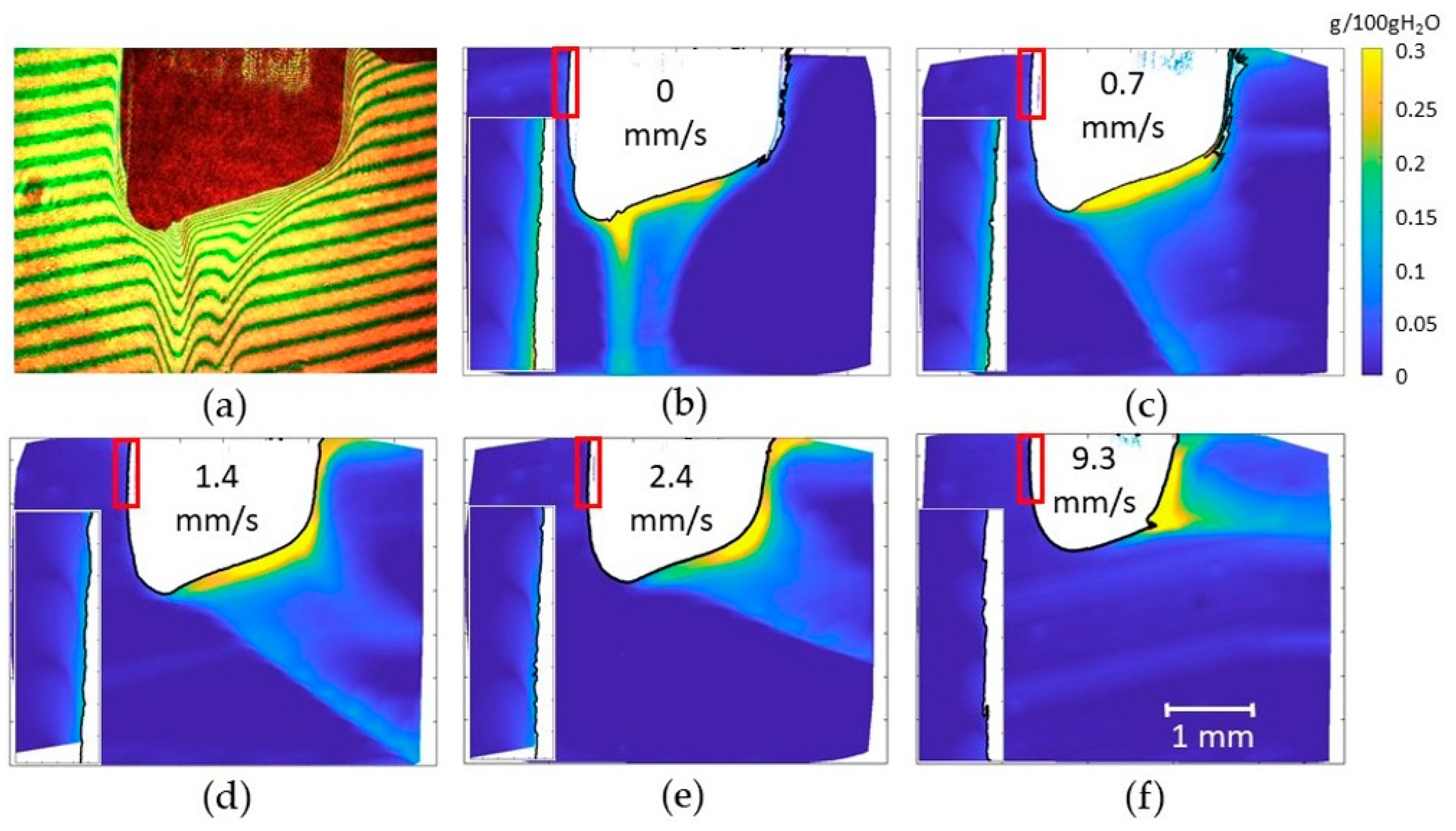
3.5. Visualisation of Concentration Fields

In order to visualize the influence of the flow on the concentration field around the crystal, interferograms recorded during the dissolution experiment described in Section 3.4 were evaluated. Images at flow rates shortly below, near and shortly above the kink point v k = 2 mm/s were selected. Figure 12 shows the concentration field at different inflow velocities for a glycine concentration of 0.21 g/g. The concentration fields calculated from the interferograms recorded with CCD1 and a large field of view support the finding that natural convection is important for the mass transfer at low flow velocities. At v = 0 mm/s (Figure 12b), natural convection clearly dominates the mass transfer. The dissolved glycine diffuses unevenly in the solvent, but the glycine-enriched solution (surplus of concentration: 0.0015 g/g) sinks down because of its higher density in comparison to the bulk. Nevertheless, the high-resolution insert of CCD2 shows that a stable diffusive layer was formed on the crystal surface exposed to the flow. As the flow rate increases (Figure 12c–f), the dissolved glycine is driven further and further downstream until the area of increased concentration is finally located entirely behind the crystal. In the area of transition from natural to forced convection-dominated mass transfer, the angle of the glycine flux is approx. 45° to the flow direction, i.e., the sinking speed at natural convection equals the flow speed. As already reported in Section 3.4, the concentration fields obtained from the images of CCD2 show that the diffusive layer is rather unaffected by low flow rates. When forced convection becomes increasingly important for mass transfer, the thickness of the diffusive boundary layer decreases rapidly with increased flow velocity and is no longer observable above 9.3 mm/s.
The concentration fields thus confirm the statements about the dominating mass transfer mechanism made in Section 3.3 on the basis of the dimensionless characteristic numbers. Note that the reasoning based on the Sherwood number requires measurements at different flow rates. The concentration field, on the other hand, visualizes the mass transfer at a certain flow rate in a single experiment. In addition, it shows the influence of the flow on the diffusive boundary layer, which is particularly essential when natural convection becomes less important for mass transfer in the case of small or less soluble crystals. Furthermore, temporally and spatially resolved 2D concentration fields can also be generated by model-based calculations that take into account fluid mechanics, diffusion and also face-specific disintegration rates. A comparison with our experimentally determined concentration fields allows the validation of the parameters used.

4. Conclusions and Outlook

We present an optical method that allows the determination of the face-specific dissolution rates of a single crystal that is subjected to a defined flow. At the same time, the concentration field around the crystal is measured with a Mach–Zehnder interferometer.
For the feasibility study presented here, we chose α-glycine in an aqueous solution as the test substance. Sherwood numbers calculated from the measured face-displacement velocities allow the identification of the dominant mass transfer mechanism. In our experiments, natural convection dominates the glycine mass transfer in the low-velocity range. However, diffusive mass transfer is expected to gain influence and limit the dissolution for smaller crystals or for less soluble substances. The concentration fields support the statements concerning the mass transfer mechanism. High-resolution images visualize the diffusive boundary layer and show its decrease with increased flow velocity. Images with a large field of view visualize natural and forced convection and the point of transition between the dominating regimes.
The applicability of our method for glycine dissolution has been successfully demonstrated. It should also be transferable to crystals of other sizes, shapes and especially to less soluble crystals. If necessary, the width of the flow cell or the field of view of the cameras must be adjusted. In the planned investigation of poorly soluble APIs, we want to confirm the prediction of the diffusion limitation at low flow velocities and we expect to recognize the onset of a disintegration limitation when the flow velocity increases.
Our method provides the outline of the crystal projection along with spatially and time-resolved concentration fields. It can therefore be used for the experimental validation of computational fluid dynamics simulations of a dissolution process. With regard to the time and cost factors in drug development, this is particularly important if disintegration rates modeled in silico are used for the simulation.

Author Contributions

Conceptualization, C.E., F.L. and H.B.; dissolution experiments, C.E.; crystal facets identification, S.A.S.; data curation, C.E.; writing—original draft preparation, C.E.; writing—review and editing, C.E., S.A.S., F.L. and H.B.; supervision, H.B.; funding acquisition, H.B. All authors have read and agreed to the published version of the manuscript.

Funding

This research was funded by the Deutsche Forschungsgemeinschaft (DFG), grant number BR2035/8-2.

Data Availability Statement

The data presented in this study are available on request from the corresponding author.

Conflicts of Interest

The authors declare no conflict of interest.

Appendix A

Table A1. Part list of the optical set-up.
Mach–Zehnder Interferometer: Visualization of Concentration Field
light sourcelaser head HeNe 633-15 P (Qioptiq Photonics GmbH & Co. KG,
Königsallee 23, 37081 Göttingen, Germany)
beam expanderbeamexpander 10x (Qioptiq Photonics GmbH & Co. KG,
Königsallee 23, 37081 Göttingen, Germany)
beam splittersbeamsplitter cube VIS; N-BK7; L = 16 (Qioptiq Photonics GmbH & Co. KG, Königsallee 23, 37081 Göttingen, Germany)
Crystal Imaging
light sourceLaser Head HeNe 543-2 (Qioptiq Photonics GmbH & Co. KG,
Königsallee 23, 37081 Göttingen, Germany)
beam expanderbeamexpander 10x (Qioptiq Photonics GmbH & Co. KG,
Königsallee 23, 37081 Göttingen, Germany)
Image Acquisition
CCD1U3-3560XCP-C-HQ (IDS Imaging Development Systems GmbH,
Dimbacher Strasse 10, 74182 Obersulm, Germany)
lens of CCD1Canon Macro Lens FL 1:3.5/50 mm (Canon Deutschland GmbH, Europark Fichtenhain A10, 47807 Krefeld, Germany) with adapter Fotodiox-Canon FD lens to C-mount (Vision Dimension GmbH, Am Kiel-Kanal 1, 24106 Kiel, Germany)
CCD2UI-2280SE-C (IDS Imaging Development Systems GmbH,
Dimbacher Strasse 10, 74182 Obersulm, Germany)
lens of CCD2Optem Zoom 70XL (0.75×–5×), selected magnification 2.0 (Polytec GmbH, Polytec-Platz 1-7, 76337 Waldbronn, Germany)
mirrorplano mirror Pl. Mirror RAL; D = 22.4 × 31.5 oval; d = 3.5; L/2 (Qioptic Photonics GmbH & Co. KG, Königsallee 23, 37081 Göttingen, Germany)
Table A2. Part list of the fluidmechanical set-up.
Flow-Through Cell
channel dimension110 mm × 24 mm × 5 mm
windowssoda lime glass, 76 mm × 26 mm × 1 mm (Menzel-Gläser, VWR International GmbH, Fraunhoferstr. 11, 85737 Ismaning, Germany), optical accessible: 70 mm × 22 mm
tube connectionsinner diameter: 4 mm
gluedual component epoxy adhesive (UHU plus endfest,
Pumps
syringe pump
0.5 to 17.5 mL/min
Atlas Syringe Pump (Syrris Ltd., Unit 3, Anglian Business Park, Royston, Herts, SG8 5TW, UK)
2.5 mL/l syringe, continuous mode
gear pump
27 to 800 mL/min
Verdergear VGS04027 with built-in frequency converter (Verder Deutschland GmbH & Co. KG, Retsch-Allee 1-5, 42781 Haan, Germany)
Tubing
silicone tubesRotilabo silicone standard design 5.0 mm, 8.0 mm (Carl Roth GmbH + Co. KG, Schoemperlenstr. 3-5, 76185 Karlsruhe, Germany)
Temperature Control
water bathThermo Electron Haake Phönix II Type P1 (Thermo Haake, Dieselstr. 4, 76227 Karlsruhe, Germany)
heat exchangeraluminum block,
contact areas: 40 cm2 to solvent, 200 cm2 to bathwater
temperature measurementGreisinger GMH 3230 with thermocouple GTF 3000 (GHM Messtechnik GmbH, Hans-Sachs-Str. 26, 93128 Regenstauf, Germany)
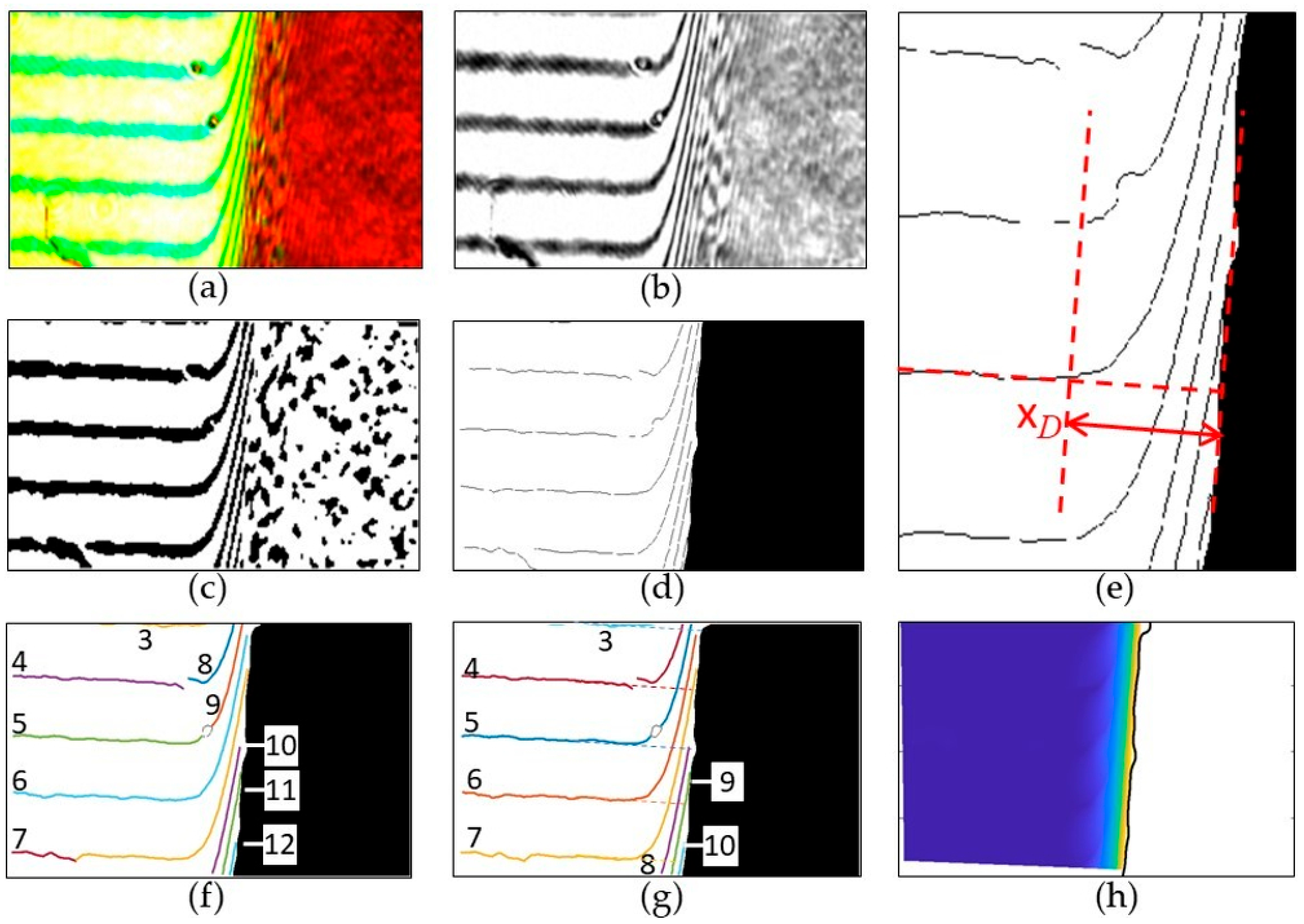
Appendix B

The image processing procedure for the determination of the crystal outline is described in Table A3. The most important MATLAB commands with the input parameters are given for each step. Figure A1 illustrates the effect of the image processing steps.
The image processing procedure for the determination of the concentration field is described in Table A4. Figure A2 illustrates the effect of the image processing steps. Up to now, not all steps are fully automated. Steps 8, 11, 12 and 14 are manual actions.
Table A3. Image processing procedure to find the crystal outline.
StepActionMATLAB Command
1select a region of interest (ROI)
see Figure A1a
2restrict to green channel
see Figure A1b
ROI = ROI(:,:,2)
3smooth to reduce image noiseROI = imgaussfilt(ROI,3)
4determinate global image thresholdT = graythresh(ROI)
5binarize to identify the crystal
see Figure A1c
ROI = imbinarize(ROI,T)
6morphological opening to
remove small dropouts and smooth the crystal outline
ROI = imopen(ROI,strel(‘disk’,20)
7remove artifacts outside the crystal, see Figure A1dROI = bwselect(~ROI,x,y)
(x,y: coordinates of a pixel inside the crystal)
8create the crystal outline
see Figure A1e
OUTLINE = bwmorph(ROI,‘remove’)
Table A4. Image processing procedure for the determination of the concentration field.
StepActionMATLAB Command
1Select a region of interest (ROI), see Figure A2a
2Restrict to red channel
see Figure A2b
ROI = ROI(:,:,1)
3Smooth to reduce image noise ROI = imgaussfilt(ROI,3)
5Binarize with adaptive threshold, see Figure A2c ROI = imbinarize(ROI,‘adaptive’,…
   ‘ForegroundPolarity’,‘dark’,‘Sensitivity’,0.5);
6Mask with segmented crystal
see
ROI = or(ROI, MASK)
7Shrink the fringes to lines
see Figure A2d
FRINGES = bwskel(~ROI,‘MinBranchLength’,40)
8Determine the thickness of the diffusion layer according to the method shown in Figure A2e
9Remove branchpoints to get clear fringesPOINT = bwmorph(FRINGES,‘Branchpoints’);
FRINGES = and(FRINGES,~POINT);
10Remove line segments
shorter than 5% of the longest (index IX)
LINES = bwconncomp(FRINGES,8);
STATS = regionprops(LINES,…
      ‘MajorAxisLength’);
LONG = max([STATS.MajorAxisLength]);
IX = find([STATS.MajorAxisLength] >…
    0.05×LONG);
11The remaining lines are numbered (Figure A2f). Manual renumbering assigns the same number to all line segments belonging to one fringe
12Sort the lines in ascending order (Figure A2g). The assigned number indicates the local phase shift between test and reference beam as a multiple of 2π
13Generate a phase shift field in the entire unmasked region by interpolationF0 = scatteredInterpolant(X,Y,M,…
     ’natural’,’none’);
14Select a region unaffected by the crystal
15Fit linear functions to the fringes in the unaffected
region; extrapolate to the rest of the unmasked area keeping the assigned number,
see Figure A2g, dashed lines
polyfit(X,Y,1)
16Generate the hypothetical unaffected phase shift field F1 = scatteredInterpolant(X,Y,M,…
     ’natural’,’none’);
17Calculate the concentration field (Figure A2h) using Equations (2) and (3)
Figure A1. Image processing of the green channel images: (a) original image, (b) green channel, (c) binarized image, (d) segmented crystal after morphological opening, (e) crystal outline.
Crystals 13 00315 g0a1
Figure A2. Image processing of the red channel images: (a) original image, (b) red channel, (c) binarized image, (d) masked crystal and skeletonized fringes, (e) determination of diffusive layer thickness, (f) selected fringe segments, (g) interference fringes with assigned phase shifts as a multiple of 2 π together with the fringes of a hypothetical homogeneous concentration field (dashed lines) and (h) calculated concentration field.
Crystals 13 00315 g0a2

References

  1. Farid, S.S.; Baron, M.; Stamatis, C.; Nie, W.; Coffman, J. Benchmarking biopharmaceutical process development and manufacturing cost contributions to R&D. MAbs 2020, 12, 1754999. [Google Scholar] [PubMed]
  2. Simoens, S.; Huys, I. R&D costs of new medicines: A landscape analysis. Front. Med. 2021, 8, 1891. [Google Scholar]
  3. Alqahtani, M.S.; Kazi, M.; Alsenaidy, M.A.; Ahmad, M.Z. Advances in oral drug delivery. Front. Pharmacol. 2021, 12, 618411. [Google Scholar] [CrossRef] [PubMed]
  4. Domingos, S.; André, V.; Quaresma, S.; Martins, I.C.; Minas da Piedade, M.F.; Duarte, M.T. New forms of old drugs: Improving without changing. J. Pharm. Pharmacol. 2015, 67, 830–846. [Google Scholar] [CrossRef]
  5. Uddin, R.; Saffoon, N.; Sutradhar, K.B. Dissolution and dissolution apparatus: A review. Int. J. Curr. Biomed. Pharm. Res. 2011, 1, 201–207. [Google Scholar]
  6. Mann, J.; Dressman, J.; Rosenblatt, K.; Ashworth, L.; Muenster, U.; Frank, K.; Hutchins, P.; Williams, J.; Klumpp, L.; Wielockx, K.; et al. Validation of dissolution testing with biorelevant media: An OrBiTo study. Mol. Pharm. 2017, 14, 4192–4201. [Google Scholar] [CrossRef]
  7. Berben, P.; Ashworth, L.; Beato, S.; Bevernage, J.; Bruel, J.-L.; Butler, J.; Dressman, J.; Schäfer, K.; Hutchins, P.; Klumpp, L.; et al. Biorelevant dissolution testing of a weak base: Interlaboratory reproducibility and investigation of parameters controlling in vitro precipitation. Eur. J. Pharm. Biopharm. 2019, 140, 141–148. [Google Scholar] [CrossRef]
  8. Kulkarni, A.; Bachhav, R.; Hol, V.; Shete, S. Co-crystals of active pharmaceutical ingredient-ibuprofen lysine. Int. J. Appl. Pharm. 2020, 12, 22–32. [Google Scholar] [CrossRef]
  9. Ambasana, M.A.; Kapuriya, N.P.; Ambasana, P.A.; Bhalodia, J.J.; Bapodra, A.H. Biorelevant dissolution studies of platelet aggregation inhibitor: Ticagrelor hydrochloride and its co-crystal with sodium salt of Aspirin. Indian J. Chem. Technol. 2022, 29, 99–103. [Google Scholar] [CrossRef]
  10. Cammarn, S.R.; Sakr, A. Predicting dissolution via hydrodynamics: Salicylic acid tablets in flow through cell dissolution. Int. J. Pharm. 2000, 201, 199–209. [Google Scholar] [CrossRef]
  11. Emara, L.H.; Emam, M.F.; Taha, N.F.; El-ashmawy, A.A.; Mursi, N.M. In-vitro dissolution study of meloxicam immediate release products using flow through cell (USP apparatus 4) under different operational conditions. Int. J. Pharm. Pharm. Sci. 2014, 6, 254–260. [Google Scholar]
  12. Medina-López, J.R.; Sánchez-Badajos, S.; Carreto-Jiménez, R.M.; García-Hernández, P.; Contreras-Jiménez, J.M. Comparative in vitro dissolution studies of fixed-dose combination formulations: Analgesic tablets of acetaminophen/caffeine. Int. J. Res. Pharm. Sci. 2021, 12, 1063–1073. Available online: https://ijrps.com/index.php/home/article/view/79/ (accessed on 29 January 2023).
  13. Greiner, M.; Choscz, C.; Eder, C.; Elts, E.; Briesen, H. Multiscale modeling of aspirin dissolution: From molecular resolution to experimental scales of time and size. Crystengcomm 2016, 18, 5302–5312. [Google Scholar] [CrossRef] [Green Version]
  14. Shaw, L.R.; Irwin, W.J.; Grattan, T.J.; Conway, B.R. The effect of selected water-soluble excipients on the dissolution of paracetamol and ibuprofen. Drug Dev. Ind. Pharm. 2005, 31, 515–525. [Google Scholar] [CrossRef]
  15. Sugano, K. A simulation of oral absorption using classical nucleation theory. Int. J. Pharm. 2009, 378, 142–145. [Google Scholar] [CrossRef]
  16. Kostewicz, E.S.; Wunderlich, M.; Brauns, U.; Becker, R.; Bock, T.; Dressman, J.B. Predicting the precipitation of poorly soluble weak bases upon entry in the small intestine. J. Pharm. Pharmacol. 2004, 56, 43–51. [Google Scholar] [CrossRef]
  17. Elts, E.; Greiner, M.; Briesen, H. In Silico Prediction of Growth and Dissolution Rates for Organic Molecular Crystals: A Multiscale Approach. Crystals 2017, 7, 288. [Google Scholar] [CrossRef]
  18. Dogan, B.; Schneider, J.; Reuter, K. In silico dissolution rates of pharmaceutical ingredients. Chem. Phys. Lett. 2016, 662, 52–55. [Google Scholar] [CrossRef]
  19. Offiler, C.A.; Cruz-Cabeza, A.J.; Davey, R.J.; Vetter, T. Crystal Growth Cell Incorporating Automated Image Analysis Enabling Measurement of Facet Specific Crystal Growth Rates. Cryst. Growth Des. 2021, 22, 2837–2848. [Google Scholar] [CrossRef]
  20. Shekunov, B.Y.; Grant, D.J. In situ optical interferometric studies of the growth and dissolution behavior of paracetamol (acetaminophen). 1. Growth kinetics. J. Phys. Chem. B 1997, 101, 3973–3979. [Google Scholar] [CrossRef]
  21. Goudarzi, N.M.; Samaro, A.; Vervaet, C.; Boone, M.N. Development of Flow-Through Cell Dissolution Method for In Situ Visualization of Dissolution Processes in Solid Dosage Forms Using X-ray μCT. Pharmaceutics 2022, 14, 2475. [Google Scholar] [CrossRef] [PubMed]
  22. Østergaard, J.; Lenke, J.; Jensen, S.S.; Sun, Y.; Ye, F. UV imaging for in vitro dissolution and release studies: Initial experiences. Dissolution Technol. 2014, 21, 27–38. [Google Scholar] [CrossRef]
  23. Adobes-Vidal, M.; Shtukenberg, A.G.; Ward, M.D.; Unwin, P.R. Multiscale visualization and quantitative analysis of L-cystine crystal dissolution. Cryst. Growth Des. 2017, 17, 1766–1774. [Google Scholar] [CrossRef]
  24. Verma, S.; Shlichta, P.J. Imaging techniques for mapping solution parameters, growth rate, and surface features during the growth of crystals from solution. Prog. Cryst. Growth Charact. Mater. 2008, 54, 1–120. [Google Scholar] [CrossRef]
  25. Srivastava, A.; Muralidhar, K.; Panigrahi, P. Optical imaging and three dimensional reconstruction of the concentration field around a crystal growing from an aqueous solution: A review. Prog. Cryst. Growth Charact. Mater. 2012, 58, 209–278. [Google Scholar] [CrossRef]
  26. Eder, C.; Briesen, H. Interferometric Probing of Physical and Chemical Properties of Solutions: Noncontact Investigation of Liquids. Annu. Rev. Chem. Biomol. Eng. 2022, 13, 99–121. [Google Scholar] [CrossRef]
  27. Otálora, F.; Novella, M.L.; Gavira, J.A.; Thomas, B.R.; Ruiz, J.M.G. Experimental evidence for the stability of the depletion zone around a growing protein crystal under microgravity. Acta Crystallogr. Sect. D Biol. Crystallogr. 2001, 57, 412–417. [Google Scholar] [CrossRef]
  28. Yin, D.; Inatomi, Y.; Kuribayashi, K. Study of lysozyme crystal growth under a strong magnetic field using a Mach–Zehnder interferometer. J. Cryst. Growth 2001, 226, 534–542. [Google Scholar] [CrossRef]
  29. Zhao, J.; Miao, H.; Duan, L.; Kang, Q.; He, L. The mass transfer process and the growth rate of NaCl crystal growth by evaporation based on temporal phase evaluation. Opt. Lasers Eng. 2012, 50, 540–546. [Google Scholar] [CrossRef]
  30. Eder, C.; Choscz, C.; Müller, V.; Briesen, H. Jamin-interferometer-setup for the determination of concentration and temperature dependent face-specific crystal growth rates from a single experiment. J. Cryst. Growth 2015, 426, 255–264. [Google Scholar] [CrossRef]
  31. Adawy, A.; Marks, K.; de Grip, W.J.; van Enckevort, W.J.P.; Vlieg, E. The development of the depletion zone during ceiling crystallization: Phase shifting interferometry and simulation results. Crystengcomm 2013, 15, 2275–2286. [Google Scholar] [CrossRef]
  32. Hou, W.; Kudryavtsev, A.; Bray, T.; DeLucas, L.; Wilson, W. Real time evolution of concentration distribution around tetragonal lysozyme crystal: Case study in gel and free solution. J. Cryst. Growth 2001, 232, 265–272. [Google Scholar] [CrossRef]
  33. Fukui, K.; Nakajima, M. Diffusion processes near the crystal surface in growth and dissolution. J. Chem. Eng. Jpn. 1985, 18, 27–32. [Google Scholar] [CrossRef] [Green Version]
  34. Divya, H.; Reddy, G.R.; Sobhan, C.B.P. Digital Interferometric Measurement of Forced Convection Fields in Compact Channels. Int. J. Optomechatron. 2015, 9, 9–34. [Google Scholar] [CrossRef]
  35. Van Dam, J.; Mischgofsky, F. The application of a new, simple interference technique to the determination of growth concentration gradients of the layer perovskite NH3(CH2)3NH3CdCl4. J. Cryst. Growth 1987, 84, 539–551. [Google Scholar] [CrossRef]
  36. Han, G.; Chow, P.S.; Tan, R.B.H. Salt-dependent growth kinetics in glycine polymorphic crystallization. Crystengcomm 2016, 18, 462–470. [Google Scholar] [CrossRef]
  37. Marsh, R.E. A refinement of the crystal structure of glycine. Acta Crystallogr. 1958, 11, 654–663. [Google Scholar] [CrossRef]
  38. Kovacevic, T.; Reinhold, A.; Briesen, H. Identifying faceted crystal shape from three-dimensional tomography data. Cryst. Growth Des. 2014, 14, 1666–1675. [Google Scholar] [CrossRef]
  39. Nernst, W. Theorie der Reaktionsgeschwindigkeit in heterogenen Systemen. Z. Phys. Chem. 1904, 47, 52–55. [Google Scholar] [CrossRef]
  40. Mullin, J.W. Crystallization; Elsevier: Amsterdam, The Netherlands, 2001. [Google Scholar]
  41. Onuma, K.; Tsukamoto, K.; Sunagawa, I. Role of buoyancy driven convection in aqueous solution growth; A case study of Ba(NO3)2 crystal. J. Cryst. Growth 1988, 89, 177–188. [Google Scholar] [CrossRef]
  42. Han, G.; Chow, P.S.; Tan, R. Understanding the Salt-Dependent Outcome of Glycine Polymorphic Nucleation. Pharmaceutics 2021, 13, 262. [Google Scholar] [CrossRef] [PubMed]
  43. Bermingham, S.K. A Design Procedure and Predictive Models for Solution Crystallisation Processes; Delft University of Technology, TU Delft: Delft, The Netherlands, 2003. [Google Scholar]
  44. Bovington, C.H.; Jones, A.L. Tracer study of the kinetics of dissolution of barium sulphate. Trans. Faraday Soc. 1970, 66, 764–768. [Google Scholar] [CrossRef]
  45. Mullin, J.W.; Garside, J. Crystallization of aluminium potassium sulphate: A study in the assessment of crystallizer design data. Part I: Single crystal growth rates. Trans. Inst. Chem. Eng. 1967, 45, T285–T290. [Google Scholar]
  46. Bomio, P.; Bourne, J.; Davey, R. The growth and dissolution of hexamethylene tetramine in aqueous solution. J. Cryst. Growth 1975, 30, 77–85. [Google Scholar] [CrossRef]
  47. Pohar, A.; Likozar, B. Dissolution, nucleation, crystal growth, crystal aggregation, and particle breakage of amlodipine salts: Modeling crystallization kinetics and thermodynamic equilibrium, scale-up, and optimization. Ind. Eng. Chem. Res. 2014, 53, 10762–10774. [Google Scholar] [CrossRef]
  48. Ninni, L.; Meirelles, A.J.A. Water activity, pH and density of aqueous amino acids solutions. Biotechnol. Prog. 2001, 17, 703–711. [Google Scholar] [CrossRef]
  49. Devine, W.; Lowe, B.M. Viscosity B-coefficients at 15 and 25 °C for glycine, β-alanine, 4-amino-n-butyric acid, and 6-amino-n-hexanoic acid in aqueous solution. J. Chem. Soc. A Inorg. Phys. Theor. 1971, 2113–2116. [Google Scholar] [CrossRef]
  50. Ma, Y.; Zhu, C.; Ma, P.; Yu, K.T. Studies on the diffusion coefficients of amino acids in aqueous solutions. J. Chem. Eng. Data 2005, 50, 1192–1196. [Google Scholar] [CrossRef]
Figure 1. Experimental set-up showing the Mach–Zehnder interferometer with the integrated flow-through cell.
Crystals 13 00315 g001
Figure 2. Flow-through cell with the crystal in the center of the channel and marked flow direction.
Crystals 13 00315 g002
Figure 3. Typical α-glycine crystal: (a) photography, (b) µ-CT image with indexed crystal facets.
Crystals 13 00315 g003
Figure 4. Determination of the face displacement velocity: (a) original image, (b) crystal outline and (c) determination of the face displacement velocity.
Crystals 13 00315 g004
Figure 5. Extraction of the concentration field (a) original image, (b) determination of diffusive layer thickness and (c) calculated concentration field.
Crystals 13 00315 g005
Figure 6. Refractive index of glycine solutions at 25 °C.
Crystals 13 00315 g006
Figure 8. Development of crystal shape during a dissolution experiment with v = 92 mm/s and c = 0.16 g/g (a) before filling, (b) first image after filling, (c) last image, taken after 6.5 min.
Crystals 13 00315 g008
Figure 9. Face displacement velocity of the (110) glycine facet under forced convection. Values at stagnant flow (oval marking) are plotted at v = 0.01 mm/s to show them in the logarithmic representation.
Crystals 13 00315 g009
Figure 10. Plot of S h against R e 1 / 2   ·   S c 1 / 3 . The dashed horizontal lines for Re < 30 (v < 2 mm/s) show S h , calculated from Equation (10) for the three investigated concentrations. The dashed black line represents the fit curve for Re > 30, given by Equation (12).
Crystals 13 00315 g010
Figure 11. Thickness of the diffusive layer at the (110) glycine facet in moving glycine solutions. Values at stagnant flow (oval marking) are entered at v = 0.01 mm/s to show them in the logarithmic representation.
Crystals 13 00315 g011
Figure 12. Dissolution in the 0.21 g/g solution. The inflow is from the left. (a) Original image at v = 0 mm/s. (bf) Concentration fields at increasing velocity (indicated in each image). The inserts show the marked section of the crystal–liquid interface with the resolution of CCD2.
Crystals 13 00315 g012
Disclaimer/Publisher’s Note: The statements, opinions and data contained in all publications are solely those of the individual author(s) and contributor(s) and not of MDPI and/or the editor(s). MDPI and/or the editor(s) disclaim responsibility for any injury to people or property resulting from any ideas, methods, instructions or products referred to in the content.

