Dynamic Analysis of Multilayered Piezoelectric Quasicrystal Three-Dimensional Sector Plates with Imperfect Interfaces

Abstract

Piezoelectric quasicrystals have attracted extensive attention due to their unique physical and mechanical properties. This paper studies the dynamic response of multilayered two-dimensional decagonal piezoelectric quasicrystal sector plates with imperfect interfaces. Based on the quasicrystal linear elasticity, partial differential state equations along the thickness direction are derived by using the state-space method. Then, by virtue of the differential quadrature method and the Fourier series expansions, this boundary-value problem with mixed boundary conditions and imperfect interfaces is solved. In addition, via the joint coupling matrix, the field quantities in the interior of the structure are connected to those on the external surfaces with numerical instability. Finally, parameter studies on the effects of angular spans, imperfect interfaces, and mixed boundary conditions are numerically investigated where the dimensionless frequencies and modes are exhibited.

1. Introduction

Quasicrystal (QC) was discovered by Shechtman [1] in the electron diffraction pattern of rapidly frozen Al-Mn alloy in 1982. QCs have excellent physical and mechanical properties such as high hardness, high conductivity, low thermal conductivity, and photoconductivity due to their unique atomic configuration [2,3]. These properties make QCs widely useful in engineering as composite strengthening phase, thermal barrier coating, and solar thin film [4,5,6]. As such, QCs have attracted great attention of researchers in many fields, such as mathematics, material science, crystallography, and physics. QCs can be divided into one-dimensional (1D), two-dimensional (2D), and three-dimensional (3D) QCs according to the numbers of the quasiperiodic directions [7]. In the 2D QCs studied in this paper, the arrangement of atoms is quasiperiodic in two directions and periodic in the other direction. To understand the deformation behavior of QCs and describe their deformation process, QC elasticity is needed. The QC elasticity theory originated from condensed matter physics rather than traditional mechanics. According to Landau’s density wave theory, there are two displacement fields in QCs: the phonon field and the phason field. Based on Landau’s elementary excitation theory and the symmetry-breaking principle of condensed matter, Bak [8] developed the QC elasticity theory, whilst Lubensky [9] developed the elasticity of QCs based on the elementary excitation theory.

As for the dynamics of QCs, different with the certainty of statics, due to its unclear physical phenomenon of the phason field, there are some arguments on the dynamic behavior of QCs. Lubensky et al. [10] claimed that the phonon field and the phason field played different roles in the dynamic behavior of QCs because the phason field was insensitive to spatial translations, and the phasons were diffusive with very large diffusion times rather than propagating. Based on this, Lubensky et al. [9,10] proposed the hydrodynamics model of QCs. On the other hand, Bak [8,11] pointed out that the phonon field and the phason field behaved similarly in dynamics, and both followed the acoustic modes. Based on this point, Ding et al. [12] first discussed the motion equation of QCs where the law of momentum conservation held for both phonons and phasons, i.e., both the phonons and phasons are represented by wave propagations, named the elastodynamic model of wave type [13], and the equation of motion for both phonons and phasons followed the wave type. However, there was another voice that argued that the phonons followed the wave type while the phasons followed the diffusion type. Based on this point of view, Fan et al. [14] and Rochal and Lorman [15,16] compromised, respectively, the hydrodynamic model and the elastodynamic model to generate the elasto-hydrodynamics model of QCs. In this model, the equation of motion for phonons followed the wave type, while those for the phasons followed the diffusion type by replacing the mass density with the kinematic coefficient of the phason field. After that, Agiasofitou and Lazar [17] unified the elastodynamic model of wave type and the elasto-hydrodynamic model to establish the elastodynamic model of the wave-telegraph type. In this model, they claimed that the phonons were represented by undamped waves, while the phasons were represented by waves damped in time and propagating with finite velocity. Thus, the equation of motion for phonons followed the wave type, while those for the phasons followed the telegraph type. To sum up, these models based on different hypotheses were used by many researchers to collect the dynamic behavior of QCs. However, due to the lack of proper experimental data, all of these existing models possessed their reasons. In this paper, we used the elastodynamic model with the wave type to study the dynamic behavior of QCs.

Layered composites can be used to design the strength and stiffness of the involved structures according to the load requirements. As such, layered composites have become the main structural form of composites in industrial applications, while QCs, due to their material properties, usually serve as the thin film, coating layers, or reinforcement phase on advanced structures. Their unique properties can be used to improve the hardness and stiffness of the composites [18,19]. As such, layered QC composites have become an attractive topic of research. By extending the pseudo-Stroh formalism, Pan and Heyliger [20] and Yang et al. [21] found exact solutions of multilayered multiferroics plates and 2D decagonal QC plates with simply supported boundary conditions. Guo et al. [22,23,24] obtained the analytical solutions for free and forced vibrations and static bending deformation of 1D QC nanoplates. Huang et al. [25] used the state-space method in their dynamic analysis of multilayered 2D piezoelectric QC (PQC) cylindrical shells filled with compressible fluid. Li et al. [26] deduced QC elasticity theory and elastodynamics for wave propagation. However, the pseudo-Stroh formalism [27,28] and the state-space method [29,30] are limited to the QC plates with simply supported boundary conditions. Plates with clamped or mixed boundary conditions cannot be solved by these two approaches.

Typically, the differential quadrature method (DQM) is employed to address static response and free vibration problems in plates subjected to arbitrary boundary conditions. In past decades, DQM was proven to be very efficient in solving differential equations with controlled boundaries or initial conditions [31]. Chen et al. [32] applied the DQM to the structural free vibration analysis of composite beams under different boundary conditions. Also via the DQM method, Lu et al. [33] carried out the static analysis of composite beams with complex boundaries and introduced a new propagator matrix method to ensure numerical stability. Zhou et al. [34] used DQM along with the state-space method to derive the natural frequencies of multilayered plates under multi-field couplings with complex boundary conditions. The dynamic and static problems of various crystal plates and crystal beams under different boundary conditions were also solved [35,36,37,38]. Recently, Feng et al. [39] analyzed cubic QCs with imperfect interfaces under mixed boundary conditions. While the traditional state-space method can only solve problems with simply supported boundaries, the DQM along with the state-space method used in this paper can solve the problems with arbitrary boundary conditions.

Piezoelectric material is capable of converting electrical energy into mechanical energy and vice versa. As such, they are widely used in the design of piezoelectric sensors in biomedicine and other fields [40]. Piezoelectric quasicrystal (PQC) materials combine the advantages of piezoelectric and QC materials and therefore offer superior performance compared to conventional piezoelectric materials. Huang et al. [41] analyzed the interlaminar stress of free-edge piezoelectric composite laminates. Khalid et al. [42] introduced a new loading condition when considering thermal–electric coupling and analyzed the free-edge interlaminar stress of smart composite laminates. Li et al. [43] constructed the exact solutions of 1D hexagonal QC with a piezoelectric effect.

A common assumption in the aforementioned works is that the extended displacement and traction vectors are continuous on the interface of two adjacent layers. However, most interfaces are imperfect as various damages could occur there (e.g., debonding, sliding, or cracking across the interface). So far, various imperfect interface models were proposed on heat conduction [44], piezoelectricity [45,46], and elasticity [47,48,49,50,51]. In this paper, the imperfect interface with mechanical flexibility and weak (or high) conductivity proposed by Pan et al. [52] is used and verified in the 3D analysis of multilayered 2D decagonal PQC sector plates under mixed boundary conditions. Because the interface is not perfect in elasticity and dielectric properties, it is not easy to handle. Chen et al. [53] deduced the exact solution of a simply supported multilayered orthotropic piezoelectric rectangular plate with mechanical compliance and weak dielectric conduction interface by using the state-space method under isothermal conditions. The vibration analysis of circular, annular, and fan-shaped layered structures in the generalized boundary value problem is one of the classic problems [54]. However, the reported study mainly focuses on the static response of QC laminated circular plates or cylindrical shells, while the vibration problem of the open sector plates under multi-field coupling with different angular spans is still limited.

In this paper, the dynamic analysis of a layered 2D PQC sector plate with mixed boundary conditions and imperfect interfaces is carried out. In Section 2, the governing equations for 2D PQCs are established based on QC linear elasticity, and the state equations are formulated as partial differential equations via the state-space method. These state equations are modified by using the DQM and the Fourier series expansions to meet different boundary conditions. In Section 3, the joint coupling matrix is derived to calculate the field quantities with numerical stability. In Section 4, the imperfect connection forms of the elastic field and the dielectrically weakly (highly) conducting interface are derived. In Section 5, the effects of different angle spans, imperfect conductive interfaces, and boundary conditions on 2D PQC laminated sector plates are studied. Finally, Section 6 draws the conclusions.

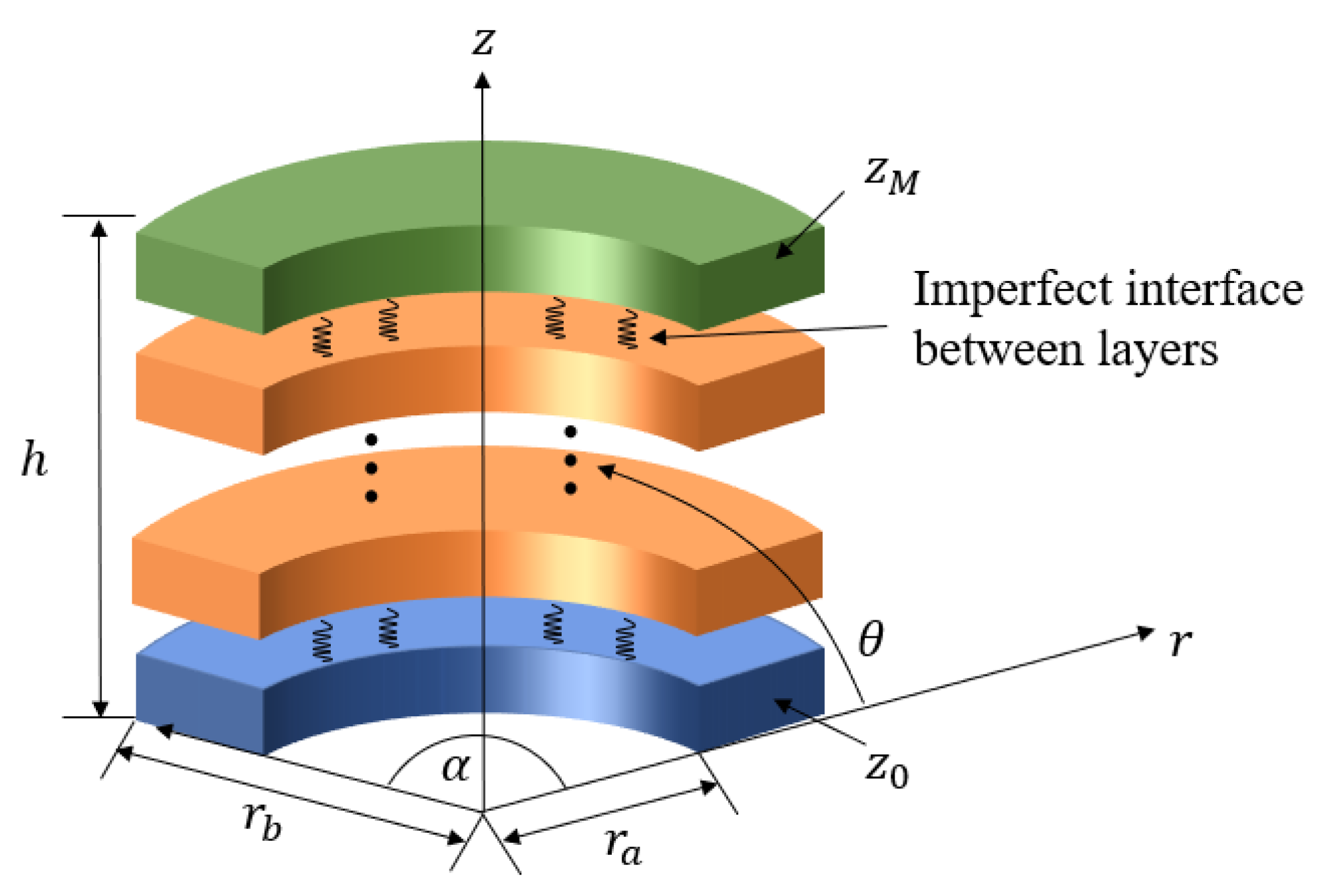
2. Problem Description

Shown in Figure 1 is the structure of a layered QC sector plate with imperfect interfaces in terms of the cylindrical coordinate system (r, θ, z). The atomic arrangement of 2D PQC is quasiperiodic along the r-θ plane and periodic along the z-direction. The total thickness is h, the inner diameter is r_a, the outer diameter is r_b, and the angle span is α. The thickness of any layer p (p = 1, 2, 3, …, M) is h_p = z_p−z_p−1 with the generalized spring model being used to simulate the imperfect interface between the layers. In this imperfect interface model, the tractions are continuous across the interface, whilst the displacements are not. According to the “spring factor” interface parameters, it is further assumed that the jump of the displacement component is proportional to the corresponding interface traction. For the dielectrically weakly conducting interface, the electric displacement is continuous, whilst the electric potential is not, with the jump in the electric potential proportional to the electric displacement. For the dielectrically highly conducting interface, the electric potential is continuous, whilst the electric displacement is not, with its discontinuity being a function of the electric potential. We further assume that the boundary conditions of the two opposite sides (θ = 0 and θ = α) of the sector plate are simply supported, while r = r_a and r = r_b can be simply supported or clamped. Additionally, for the case of free vibration, it is assumed that both elastic traction and vertical electric displacement are zero on the top and bottom surfaces of the plate.

2.1. Basic Equations

Based on the QC linear elasticity, the strain-displacement relationship of 2D PQCs is

$$\begin{array}{l}{\epsilon }_{rr}=\frac{\partial u_r}{\partial r},{\epsilon }_{\theta \theta }=\frac{\partial u_{\theta }}{r\partial \theta }+\frac{u_r}{r},{\epsilon }_{zz}=\frac{\partial u_z}{\partial z},\\ {\epsilon }_{\theta r}={\epsilon }_{r\theta }=\frac{1}{2}\left(\frac{\partial u_r}{r\partial \theta }+\frac{\partial u_{\theta }}{\partial r}-\frac{u_{\theta }}{r}\right),{\epsilon }_{rz}={\epsilon }_{zr}=\frac{1}{2}\left(\frac{\partial u_z}{\partial r}+\frac{\partial u_r}{\partial z}\right),{\epsilon }_{\theta z}={\epsilon }_{z\theta }=\frac{1}{2}\left(\frac{\partial u_{\theta }}{\partial z}+\frac{\partial u_z}{r\partial \theta }\right),\\ w_{rr}=\frac{\partial w_r}{\partial r},w_{r\theta }=\frac{\partial w_r}{r\partial \theta }-\frac{w_{\theta }}{r},w_{rz}=\frac{\partial w_r}{\partial z},w_{\theta r}=\frac{\partial w_{\theta }}{\partial r},w_{\theta \theta }=\frac{\partial w_{\theta }}{r\partial \theta }+\frac{w_r}{r},w_{\theta z}=\frac{\partial w_{\theta }}{\partial z},\\ E_r=-\frac{\partial \phi }{\partial r},E_{\theta }=-\frac{\partial \phi }{r\partial \theta },E_z=-\frac{\partial \phi }{\partial z},\end{array}$$

(1)

where ε_ij (i, j = r, θ, z) and w_kl (k, l = r, θ) are the strains in the phonon and phason fields, respectively; u_i and w_k are the displacements in the phonon and phason fields, respectively; E_i stands for the electric field; and φ represents the electric potential.

The generalized stress–strain relationship of 2D PQCs is

$$\begin{array}{l}{\sigma }_{rr}=C_{11}{\epsilon }_{rr}+C_{12}{\epsilon }_{\theta \theta }+C_{13}{\epsilon }_{zz}+R_1\left(w_{rr}+w_{\theta \theta }\right)-e_{31}{E}_z,\\ {\sigma }_{\theta \theta }=C_{12}{\epsilon }_{rr}+C_{11}{\epsilon }_{\theta \theta }+C_{13}{\epsilon }_{zz}-R_1\left(w_{rr}+w_{\theta \theta }\right)-e_{31}{E}_z,\\ {\sigma }_{zz}=C_{13}{\epsilon }_{rr}+C_{13}{\epsilon }_{\theta \theta }+C_{33}{\epsilon }_{zz}-e_{33}{E}_z,\\ {\sigma }_{\theta z}={\sigma }_{z\theta }=2C_{44}{\epsilon }_{\theta z}-e_{15}{E}_{\theta },\\ {\sigma }_{rz}={\sigma }_{zr}=2C_{44}{\epsilon }_{rz}-e_{15}{E}_r,\\ {\sigma }_{r\theta }={\sigma }_{\theta r}=2C_{66}{\epsilon }_{r\theta }-R_1{w}_{r\theta }+R_1{w}_{\theta r},\\ H_{rr}=R_1\left({\epsilon }_{rr}-{\epsilon }_{\theta \theta }\right)+K_1{w}_{rr}+K_2{w}_{\theta \theta }-d_{112}{E}_{\theta },\\ H_{\theta \theta }=R_1\left({\epsilon }_{rr}-{\epsilon }_{\theta \theta }\right)+K_1{w}_{\theta \theta }+K_2{w}_{rr}+d_{112}{E}_{\theta },\\ H_{\theta z}=K_4{w}_{\theta z},\\ H_{r\theta }=-2R_1{\epsilon }_{r\theta }+K_1{w}_{r\theta }-K_2{w}_{\theta r}-d_{112}{E}_r,\\ H_{rz}=K_4{w}_{rz},\\ H_{\theta r}=2R_1{\epsilon }_{r\theta }-K_2{w}_{r\theta }+K_1{w}_{\theta r}-d_{112}{E}_r,\\ D_r=2e_{15}{\epsilon }_{rz}+d_{112}\left(w_{r\theta }+w_{\theta r}\right)+{\xi }_{11}{E}_r,\\ D_{\theta }=2e_{15}{\epsilon }_{\theta z}+d_{112}\left(w_{rr}-w_{\theta \theta }\right)+{\xi }_{22}{E}_{\theta },\\ D_z=e_{31}\left({\epsilon }_{rr}+{\epsilon }_{\theta \theta }\right)+e_{33}{\epsilon }_{zz}+{\xi }_{33}{E}_z,\end{array}$$

(2)

where σ_ij and H_kl are the stresses in the phonon and phason fields, respectively; D_i stands for the electric displacements; C_ij, C_44, and C₆₆ = (C₁₁-C₁₂)/2 are the elastic constants in the phonon field; K₁, K₂, and K₄ represent the phason elastic constants; R₁ represents the phonon–phason coupling elastic constant; ξ_ii represent the dielectric coefficients; e₁₅, e₃₁, and e₃₃ represent the piezoelectric coefficients in the phonon field; and d₁₁₂ represents the piezoelectric coefficient in the phason field.

Based on Newton’s second law and Bak’s theory [8,11], the equations of motion of 2D PQCs in the absence of body force and electric charge densities following the elastodynamics model [12,13] can be expressed as follows:

$$\begin{array}{l}\frac{\partial {\sigma }_{rr}}{\partial r}+\frac{\partial {\sigma }_{r\theta }}{r\partial \theta }+\frac{\partial {\sigma }_{rz}}{\partial z}+\frac{{\sigma }_{rr}}{r}-\frac{{\sigma }_{\theta \theta }}{r}=\rho \frac{{\partial }^2{u}_r}{\partial t^2},\frac{\partial {\sigma }_{r\theta }}{\partial r}+\frac{\partial {\sigma }_{\theta \theta }}{r\partial \theta }+\frac{\partial {\sigma }_{\theta z}}{\partial z}+\frac{2{\sigma }_{r\theta }}{r}=\rho \frac{{\partial }^2{u}_{\theta }}{\partial t^2},\\ \frac{\partial {\sigma }_{rz}}{\partial r}+\frac{\partial {\sigma }_{z\theta }}{r\partial \theta }+\frac{\partial {\sigma }_{zz}}{\partial z}+\frac{{\sigma }_{rz}}{r}=\rho \frac{{\partial }^2{u}_z}{\partial t^2},\frac{\partial H_{rr}}{\partial r}+\frac{\partial H_{r\theta }}{r\partial \theta }+\frac{\partial H_{rz}}{\partial z}+\frac{H_{rr}-H_{\theta \theta }}{r}=\rho \frac{{\partial }^2{w}_r}{\partial t^2},\\ \frac{\partial H_{\theta r}}{\partial r}+\frac{\partial H_{\theta \theta }}{r\partial \theta }+\frac{\partial H_{\theta z}}{\partial z}+\frac{H_{r\theta }+H_{\theta r}}{r}=\rho \frac{{\partial }^2{w}_{\theta }}{\partial t^2},\frac{\partial D_r}{\partial r}+\frac{\partial D_{\theta }}{r\partial \theta }+\frac{\partial D_z}{\partial z}+\frac{D_r}{r}=0,\end{array}$$

(3)

where ρ is the mass density and t is the time.

2.2. State Equations of a Homogeneous QC Sector Plate Layer

Substituting Equation (1) into Equation (2) and combining it with Equation (3), the partial differential state equations are

$$\frac{\partial }{\partial z}{\xi }_1=D{\xi }_1,$$

(4)

where state variable ξ₁ = [u_r, u_θ, u_z, w_r, w_θ, φ, σ_zz, σ_θz, σ_rz, H_θz, H_rz, D_z]^T, in which the superscript “T” denotes the transpose of a vector or a matrix; and D stands for the state matrix.

For the electro-elastic problem of a 2D PQC sector plate, the simply supported and electrically grounded boundary conditions of the two opposite sides θ = 0 and θ = φ are

$$u_r=u_z=w_r=0,{\sigma }_{\theta \theta }=0,\phi =0.$$

(5)

Then, the general solutions of displacements, stresses, electric potential, and electric displacements satisfying Equation (5) are (for the time-harmonic case) as follows:

$$\left[\begin{array}{c}{u}_r\left(r,\theta ,z\right)\\ u_{\theta }\left(r,\theta ,z\right)\\ u_z\left(r,\theta ,z\right)\\ \begin{array}{l}{w}_r\left(r,\theta ,z\right)\\ w_{\theta }\left(r,\theta ,z\right)\end{array}\\ \phi \left(r,\theta ,z\right)\end{array}\right]={\displaystyle \sum _{n=1}^{\infty }\left[\begin{array}{c}{\tilde{u}}_r\left(r,z\right)\sin \left(p\theta \right)\\ {\tilde{u}}_{\theta }\left(r,z\right)\cos \left(p\theta \right)\\ {\tilde{u}}_z\left(r,z\right)\sin \left(p\theta \right)\\ \begin{array}{l}{\tilde{w}}_r\left(r,z\right)\sin \left(p\theta \right)\\ {\tilde{w}}_{\theta }\left(r,z\right)\cos \left(p\theta \right)\end{array}\\ \tilde{\phi }\left(r,z\right)\sin \left(p\theta \right)\end{array}\right]e^{\mathrm{i}\omega t}},\left[\begin{array}{c}{\sigma }_{rr}\left(r,\theta ,z\right)\\ {\sigma }_{\theta z}\left(r,\theta ,z\right)\\ {\sigma }_{rz}\left(r,\theta ,z\right)\\ \begin{array}{l}{H}_{\theta z}\left(r,\theta ,z\right)\\ H_{rz}\left(r,\theta ,z\right)\end{array}\\ D_z\left(r,\theta ,z\right)\end{array}\right]={\displaystyle \sum _{n=1}^{\infty }\left[\begin{array}{c}{\tilde{\sigma }}_{rr}\left(r,z\right)\sin \left(p\theta \right)\\ {\tilde{\sigma }}_{\theta z}\left(r,z\right)\cos \left(p\theta \right)\\ {\tilde{\sigma }}_{rz}\left(r,z\right)\sin \left(p\theta \right)\\ \begin{array}{l}{\tilde{H}}_{\theta z}\left(r,z\right)\cos \left(p\theta \right)\\ {\tilde{H}}_{rz}\left(r,z\right)\sin \left(p\theta \right)\end{array}\\ {\tilde{D}}_z\left(r,z\right)\sin \left(p\theta \right)\end{array}\right]}{e}^{\mathrm{i}\omega t},$$

(6)

where ω is the angular frequency, and imaginary $\mathrm{i}=\sqrt{-1}$; p = nπ/α, in which n is the half-wave number.

In the radial r-direction, we assume more general boundary conditions, including the clamped or mixed boundary conditions. Therefore, in the r-direction, the DQM is used to solve the partial differential equations. Assuming that the function f(r) is smooth and continuous in the interested r-interval, in terms of the DQM method, the approximate value of the m-order derivative of the function f(r) at r_i is

$${\frac{{\partial }^{m}f\left(r\right)}{\partial r^m}|}_{r=r_i}={\displaystyle \sum _{j=1}^N{X}_{ij}^{\left(m\right)}f\left(r_j\right)}\left(i=1,2,\dots ,N\right),$$

(7)

where $X_{ij}^{\left(m\right)}$ are the differential quadrature weight coefficients and N is the number of discrete points in the r-direction.

The form of Chebyshev-Gauss-Lobatto discrete points in a cylindrical coordinate system is given as

$$r_i=\frac{r_b-r_a}{2}\left[1-\cos \left(\frac{i-1}{N-1}\pi \right)\right]+r_{a}i=1,2,\dots N.$$

(8)

Then, the stresses, displacements, electric potential, and electric displacements in Equation (4) are expanded by the Fourier series and DQM, resulting in the following state equations:

$$\begin{array}{l}\frac{\mathrm{d}{\tilde{u}}_{ri}}{\mathrm{d}z}=-{\displaystyle \sum _{k=1}^N{X}_{ik}^{(1)}{\tilde{u}}_{zk}}-a_1{\displaystyle \sum _{k=1}^N{X}_{ik}^{(1)}{\phi }_k}+a_2{\tilde{\sigma }}_{rzi},\\ \frac{\mathrm{d}{\tilde{u}}_{\theta i}}{\mathrm{d}z}=\frac{p}{r_i}{\tilde{u}}_{zi}+a_1\frac{p}{r_i}{\tilde{\phi }}_i+a_2{\tilde{\sigma }}_{\theta zi},\\ \frac{\mathrm{d}{\tilde{u}}_{zi}}{\mathrm{d}z}=-\frac{a_4}{a_3}{\displaystyle \sum _{k=1}^N{X}_{ik}^{(1)}{\tilde{u}}_{rk}}-\frac{a_4}{a_3}\frac{1}{r_i}{\tilde{u}}_{ri}-\frac{a_4}{a_3}\frac{p}{r_i}{\tilde{u}}_{\theta i}+\frac{a_5}{a_3}{\tilde{\sigma }}_{zzi}+\frac{a_6}{a_3}{\tilde{D}}_{zi},\\ \frac{\mathrm{d}{\tilde{w}}_{ri}}{\mathrm{d}z}=\frac{1}{a_7}{\tilde{H}}_{rzi},\\ \frac{\mathrm{d}{\tilde{w}}_{\theta i}}{\mathrm{d}z}=\frac{1}{a_7}{\tilde{H}}_{\theta zi},\\ \frac{\mathrm{d}{\tilde{\phi }}_i}{\mathrm{d}z}=\frac{a_8}{a_3}{\displaystyle \sum _{k=1}^N{X}_{ik}^{(1)}{\tilde{u}}_{rk}}+\frac{a_8}{a_3}\frac{1}{r_i}{\tilde{u}}_{ri}+\frac{a_8}{a_3}\frac{p}{r_i}{\tilde{u}}_{\theta i}+\frac{a_6}{a_3}{\tilde{\sigma }}_{zzi}-\frac{a_9}{a_3}{\tilde{D}}_{zi},\\ \frac{\mathrm{d}{\tilde{\sigma }}_{rzi}}{\mathrm{d}z}=\left(\frac{a_{11}}{a_3}-a_{10}\right){\displaystyle \sum _{k=1}^N{X}_{ik}^{(2)}{\tilde{u}}_{rk}}-\left(a_{10}-a_{12}\right)\frac{1}{r_i}{\displaystyle \sum _{k=1}^N{X}_{ik}^{(1)}{\tilde{u}}_{rk}}+\\ \hspace{1em}\hspace{1em}\left(\frac{a_{11}}{a_3}-a_{12}\right){\displaystyle \sum _{k=1}^N{X}_{ik}^{(1)}\frac{1}{r_k}{\tilde{u}}_{rk}}+a_{13}\frac{p^2}{r_i^2}{\tilde{u}}_{ri}+\left(a_{10}-a_{12}\right)\frac{1}{r_i^2}{\tilde{u}}_{ri}\\ \hspace{1em}\hspace{1em}-a_{13}\frac{p}{r_i}{\displaystyle \sum _{k=1}^N{X}_{ik}^{(1)}{\tilde{u}}_{\theta k}}+\left(\frac{a_{11}}{a_3}-a_{12}\right)p{\displaystyle \sum _{k=1}^N{X}_{ik}^{(1)}\frac{1}{r_k}{\tilde{u}}_{\theta k}}\\ \hspace{1em}\hspace{1em}+\left(a_{10}-a_{12}+a_{13}\right)\frac{p}{r_i^2}{\tilde{u}}_{\theta i}-a_{14}{\displaystyle \sum _{k=1}^N{X}_{ik}^{(2)}{\tilde{w}}_{rk}}-2a_{14}\frac{1}{r_i}{\displaystyle \sum _{k=1}^N{X}_{ik}^{(1)}{\tilde{w}}_{rk}}\\ \hspace{1em}\hspace{1em}-a_{14}{\displaystyle \sum _{k=1}^N{X}_{ik}^{(1)}\frac{1}{r_k}{\tilde{w}}_{rk}}-a_{14}\frac{p^2}{r_i^2}{\tilde{w}}_{ri}-2a_{14}\frac{1}{r_i^2}{\tilde{w}}_{ri}-a_{14}\frac{p}{r_i}{\displaystyle \sum _{k=1}^N{X}_{ik}^{(1)}{\tilde{w}}_{\theta k}}\\ \hspace{1em}\hspace{1em}-a_{14}p{\displaystyle \sum _{k=1}^N{X}_{ik}^{(1)}\frac{1}{r_k}{\tilde{w}}_{\theta k}}-3a_{14}\frac{p}{r_i^2}{\tilde{w}}_{\theta i}-\frac{a_4}{a_3}{\displaystyle \sum _{k=1}^N{X}_{ik}^{(1)}{\tilde{\sigma }}_{zzk}}+\frac{a_8}{a_3}{\displaystyle \sum _{k=1}^N{X}_{ik}^{(1)}{\tilde{D}}_{zk}},\\ \frac{\mathrm{d}{\tilde{\sigma }}_{\theta zi}}{\mathrm{d}z}=-\left(a_{10}-a_{12}\right)\frac{p}{r_i}{\displaystyle \sum _{k=1}^N{X}_{ik}^{(1)}\frac{1}{r_k}{\tilde{u}}_{rk}}+a_{13}p{\displaystyle \sum _{k=1}^N{X}_{ik}^{(1)}\frac{1}{r_k}{\tilde{u}}_{rk}}-\left(\frac{a_{11}}{a_3}-a_{10}-2a_{13}\right)\frac{p}{r_i^2}{\tilde{u}}_{ri}\\ \hspace{1em}\hspace{1em}-a_{13}{\displaystyle \sum _{k=1}^N{X}_{ik}^{(2)}{\tilde{u}}_{\theta k}}-2a_{13}\frac{1}{r_i}{\displaystyle \sum _{k=1}^N{X}_{ik}^{(1)}{\tilde{u}}_{\theta k}}+a_{13}{\displaystyle \sum _{k=1}^N{X}_{ik}^{(1)}\frac{1}{r_k}{\tilde{u}}_{\theta k}}-\left(\frac{a_{11}}{a_3}-a_{10}\right)\frac{p^2}{r_i^2}{\tilde{u}}_{\theta i}\\ \hspace{1em}\hspace{1em}+2a_{13}\frac{1}{r_i^2}{\tilde{u}}_{\theta i}-a_{14}\frac{p}{r_i}{\displaystyle \sum _{k=1}^N{X}_{ik}^{(1)}{\tilde{w}}_{rk}-a_{14}p{\displaystyle \sum _{k=1}^N{X}_{ik}^{(1)}\frac{1}{r_k}{\tilde{w}}_{rk}}}-3a_{14}\frac{p}{r_i^2}{\tilde{w}}_{ri}\\ \hspace{1em}\hspace{1em}-a_{14}{\displaystyle \sum _{k=1}^N{X}_{ik}^{(2)}{\tilde{w}}_{\theta k}}-2a_{14}\frac{1}{r_i}{\displaystyle \sum _{k=1}^N{X}_{ik}^{(1)}{\tilde{w}}_{\theta k}}-a_{14}{\displaystyle \sum _{k=1}^N{X}_{ik}^{(1)}\frac{1}{r_k}{\tilde{w}}_{\theta k}}-a_{14}\frac{p^2}{r_i^2}{\tilde{w}}_{\theta i}\\ \hspace{1em}\hspace{1em}-2a_{14}\frac{1}{r_i^2}{\tilde{w}}_{\theta i}+\frac{a_4}{a_3}\frac{1}{r_i^{}}{\tilde{\sigma }}_{zzi}-\frac{a_8}{a_3}\frac{1}{r_i^{}}{\tilde{D}}_{zi},\\ \frac{\mathrm{d}{\tilde{\sigma }}_{zzi}}{\mathrm{d}z}=-{\displaystyle \sum _{k=1}^N{X}_{ik}^{(1)}{\tilde{\sigma }}_{rzk}-}\frac{1}{r_i^{}}{\tilde{\sigma }}_{rzi}-\frac{p}{r_i^{}}{\tilde{\sigma }}_{\theta zi},\end{array}$$

(9)

$$\begin{array}{l}\frac{\mathrm{d}{\tilde{H}}_{rzi}}{\mathrm{d}z}=-a_{14}{\displaystyle \sum _{k=1}^N{X}_{ik}^{(2)}{\tilde{u}}_{rk}}-a_{14}\frac{p^2}{r_i^2}{\tilde{u}}_{ri}+a_{14}{\displaystyle \sum _{k=1}^N{X}_{ik}^{(1)}\frac{1}{r_k}{\tilde{u}}_{rk}}+a_{14}\frac{p}{r_k}{\displaystyle \sum _{k=1}^N{X}_{ik}^{(1)}{\tilde{u}}_{\theta k}}\\ \hspace{1em}\hspace{1em}+a_{14}p{\displaystyle \sum _{k=1}^N\begin{array}{l}{X}_{ik}^{(1)}\frac{1}{r_k}{\tilde{u}}_{\theta k}\\ \end{array}}-a_{14}\frac{p}{r_i^2}{\tilde{u}}_{\theta i}-a_{15}{\displaystyle \sum _{k=1}^N{X}_{ik}^{(2)}{\tilde{w}}_{rk}}-\left(a_{15}-a_{16}\right)\frac{1}{r_i}{\displaystyle \sum _{k=1}^N{X}_{ik}^{(1)}{\tilde{w}}_{rk}}\\ \hspace{1em}\hspace{1em}-a_{16}{\displaystyle \sum _{k=1}^N{X}_{ik}^{(1)}\frac{1}{r_k}{\tilde{w}}_{rk}}+a_{15}\frac{p^2}{r_i^2}{\tilde{w}}_{ri}+\left(a_{15}-a_{16}\right)\frac{1}{r_i^2}{\tilde{w}}_{ri}+a_{16}\frac{p}{r_i}{\displaystyle \sum _{k=1}^N{X}_{ik}^{(1)}{\tilde{w}}_{\theta k}}\\ \hspace{1em}\hspace{1em}-a_{16}p{\displaystyle \sum _{k=1}^N{X}_{ik}^{(1)}\frac{1}{r_k}{\tilde{w}}_{\theta k}}+\left(2a_{15}-a_{16}\right)\frac{p}{r_i^2}{\tilde{w}}_{\theta i},\\ \frac{\mathrm{d}{\tilde{H}}_{\theta zi}}{\mathrm{d}z}=a_{14}\frac{p}{r_i}{\displaystyle \sum _{k=1}^N{X}_{ik}^{(1)}{\tilde{u}}_{rk}}+a_{14}p{\displaystyle \sum _{k=1}^N{X}_{ik}^{(1)}\frac{1}{r_k}{\tilde{u}}_{rk}}-a_{14}\frac{p}{r_i^2}{\tilde{u}}_{ri}-a_{14}{\displaystyle \sum _{k=1}^N{X}_{ik}^{(2)}{\tilde{u}}_{\theta k}}\\ \hspace{1em}\hspace{1em}+a_{14}{\displaystyle \sum _{k=1}^N{X}_{ik}^{(1)}\frac{1}{r_k}{\tilde{u}}_{\theta k}}-a_{14}\frac{p^2}{r_i^2}{\tilde{u}}_{\theta i}+a_{16}\frac{p}{r_i}{\displaystyle \sum _{k=1}^N{X}_{ik}^{(1)}{\tilde{w}}_{rk}}-a_{16}p{\displaystyle \sum _{k=1}^N{X}_{ik}^{(1)}\frac{1}{r_k}{\tilde{w}}_{rk}}\\ \hspace{1em}\hspace{1em}+\left(2a_{15}-a_{16}\right)\frac{p}{r_i^2}{\tilde{w}}_{ri}-a_{15}{\displaystyle \sum _{k=1}^N{X}_{ik}^{(2)}{\tilde{w}}_{\theta k}}-\left(a_{15}-a_{16}\right)\frac{1}{r_i}{\displaystyle \sum _{k=1}^N{X}_{ik}^{(1)}{\tilde{w}}_{\theta k}}\\ \hspace{1em}\hspace{1em}-a_{16}{\displaystyle \sum _{k=1}^N{X}_{ik}^{(1)}\frac{1}{r_k}{\tilde{w}}_{\theta k}}+a_{15}\frac{p^2}{r_i^2}{\tilde{w}}_{\theta i}+(a_{15}-a_{16})\frac{1}{r_i^2}{\tilde{w}}_{\theta i},\\ \frac{\mathrm{d}{\tilde{D}}_{zi}}{\mathrm{d}z}=a_{17}{\displaystyle \sum _{k=1}^N{X}_{ik}^{(2)}{\tilde{\phi }}_k}+a_{17}\frac{1}{r_i}{\displaystyle \sum _{k=1}^N{X}_{ik}^{(1)}{\tilde{\phi }}_k}-a_{18}\frac{p^2}{r_i^2}{\tilde{\phi }}_k-a_1{\displaystyle \sum _{k=1}^N{X}_{ik}^{(1)}{\tilde{\sigma }}_{rzk}}-a_1\frac{p}{r_i}{\tilde{\sigma }}_{\theta zi},\end{array}$$

(10)

where i = 1, 2, …, N, and coefficients a_m (m = 1, 2, …., 18) are listed in Equation (A1) in Appendix A.

Equations (9) and (10) represent the state equations at the endpoints when i = 1 and N. Therefore, the simply supported and clamped boundary conditions can be expressed directly by displacements, stresses, and electric potential:

$${\tilde{u}}_{\theta d}={\tilde{u}}_{zd}={\tilde{w}}_{\theta d}=0,{\tilde{\sigma }}_{rrd}=0,{\tilde{\phi }}_d=0,$$

(11)

$${\tilde{u}}_{rd}={\tilde{u}}_{\theta d}={\tilde{u}}_{zd}={\tilde{w}}_{rd}={\tilde{w}}_{\theta d}=0,{\tilde{\phi }}_d=0,$$

(12)

where d = 1 and N. To simplify presentations, the following abbreviations are introduced to express the boundary conditions of the QC sector plate: SSSS, SCSS, SSSC, and SCSC, where for example, ‘SCSS’ indicates that the boundary condition is simply supported (S) at r = r_b, clamped (C) at r = r_a, and simply supported (SS) along the edges θ = 0 and θ = α.

Therefore, in general, for the given four sets of boundary conditions: (SSSS, SCSS, SSSC, and SCSC), we can arrive at the state equation for any given layer. Taking a 2D PQC sector plate with SCSS boundary conditions as an example, the state equations are shown in Equations (A2) and (A3) in Appendix A.

As such, Equations (9) and (10) of Layer p can be simplified to matrix form:

$$\frac{\mathrm{d}}{\mathrm{d}z}{\zeta }_{}^{\left(p\right)}=P^{\left(p\right)}{\zeta }_{}^{\left(p\right)},$$

(13)

where ${\zeta }^{\left(p\right)}={\left[u_r^T,u_{\theta }^T,u_z^T,w_r^T,w_{\theta }^T,{\phi }_{}^T,{\sigma }_{zz}^T,{\sigma }_{\theta z}^T,{\sigma }_{rz}^T,H_{\theta z}^T,H_{rz}^T,D_z^T\right]}^T$ is the overall state vector and each sub-vector is composed of state variables at all discrete points (${\mathbf{u}}_r^{\mathrm{T}}={\tilde{u}}_{ri}$); and P^(p) is the coefficient matrix of Layer p.

3. General Solutions for a 2D QC Sector Plate

Since the state equations represent a system of homogeneous linear ordinary differential equations with constant coefficients, their general solutions can be obtained directly. From the general solutions, the propagation relationship of the state vectors on the top and bottom surfaces of sector plates can be obtained by combining the interface conditions between the layers.

The general solutions of the state equations Equation (13) can be expressed as

$${\zeta }_{}^{\left(p\right)}\left(z\right)=\exp \left[\left(z-z_{p-1}\right)P^{\left(p\right)}\right]{\zeta }_{}^{\left(p\right)}\left(z_{p-1}\right)\left(z_{p-1}\le z\le z_p\right),$$

(14)

where z_p-1 and z_p, respectively, represent the coordinates of the lower and upper interfaces of Layer p. If the state vector of the lower surface of Layer p is known, the state vector at any thickness position in this layer can be obtained by Equation (14). In particular, for z = z_p, we have

$${\zeta }_1^{\left(p\right)}=T^{\left(p\right)}{\zeta }_0^{\left(p\right)},$$

(15)

where ${\mathbf{T}}^{\left(p\right)}=\exp \left[{\stackrel{-}{h}}_p{\mathbf{P}}^{\left(p\right)}\right]$ is the propagator matrix of Layer p, in which ${\stackrel{-}{h}}_p=z_p-z_{p-1}$, ${\mathit{\xi }}_1^{\left(p\right)}={\mathit{\xi }}^{\left(p\right)}\left(z_p\right)$, ${\mathit{\xi }}_0^{\left(p\right)}={\mathit{\xi }}^{\left(p\right)}\left(z_{p-1}\right)$, subscripts 0 and 1 represent the lower and upper interfaces of Layer p. Similarly, for Layer p + 1, we have

$${\zeta }_1^{\left(p+1\right)}=T^{\left(p+1\right)}{\zeta }_0^{\left(p+1\right)}.$$

(16)

If we assume that these two layers are perfectly connected, then all variables are continuous at the interface

$${\zeta }_0^{\left(p+1\right)}={\zeta }_{}^{\left(p+1\right)}\left(z_p\right)={\zeta }_{}^{\left(p\right)}\left(z_p\right)={\zeta }_1^{\left(p\right)},$$

(17)

Substituting Equation (17) into Equations (15) and (16) to eliminate the state variables on their common interface z_p we obtain

$${\zeta }_1^{\left(p+1\right)}=T^{\left(p+1\right)}{T}^{\left(p\right)}{\zeta }_0^{\left(p\right)}.$$

(18)

We first assume that all the interfaces are perfect. Then, the state vectors at all interfaces can be eliminated in the same way to obtain the relationship of the state vectors on both the top and bottom surfaces of the layered plate

$${\zeta }_1^{\left(k\right)}=T{\zeta }_0^{\left(1\right)},$$

(19)

where

$$T=T^{\left(k\right)}\cdots T^{\left(p+1\right)}{T}^{\left(p\right)}\cdots T^{\left(1\right)}={\displaystyle {\prod }_{p=k}^1{T}^{\left(p\right)}},$$

(20)

and Equation (20) is called the global propagator matrix.

For convenience, Equation (19) can be written in a block matrix form as follows:

$${\left\{\begin{array}{c}U\\ \Sigma \end{array}\right\}}_1^{\left(k\right)}=\left[\begin{array}{cc}{T}_{11}& T_{12}\\ T_{21}& T_{22}\end{array}\right]{\left\{\begin{array}{c}U\\ \Sigma \end{array}\right\}}_0^{\left(1\right)},$$

(21)

where $U=\left[u_r^T,u_{\theta }^T,u_z^T,w_r^T,w_{\theta }^T,{\phi }_{}^T\right]$, $\Sigma =\left[{\sigma }_{zz}^T,{\sigma }_{\theta z}^T,{\sigma }_{rz}^T,H_{\theta z}^T,H_{rz}^T,D_z^T\right]$.

Then, from Equation (21), we have

$$U_1^{\left(k\right)}=T_{11}{U}_0^{\left(1\right)}+T_{12}{\Sigma }_0^{\left(1\right)},$$

(22)

$$T_{21}{U}_0^{\left(1\right)}={\Sigma }_1^{\left(k\right)}-T_{22}{\Sigma }_0^{\left(1\right)}.$$

(23)

Since the tractions and electric displacements on the top and bottom surfaces of the layered plate are zero for the free vibration problem, Equation (23) is simplified as

$$T_{21}{U}_0^{\left(1\right)}=0.$$

(24)

The above equations are a system of homogeneous linear equations, and the coefficient matrix is a function of the dimensionless frequency Ω. A nontrivial solution requires that the determinant of the coefficient matrix in Equation (24) be zero, i.e.,

$$\left|T_{21}\right|=0.$$

(25)

For the solved dimensionless frequency Ω from Equation (25), the corresponding eigenvectors (namely, the eigenmode of each state vector) can be obtained from Equation (19).

For the forced vibration problem, the top surface of the QC sector plate is subjected to a uniform normal mechanical excitation, namely

$$z=h:{\tilde{\sigma }}_{zz}={\sigma }_0{e}^{i\omega t},{\tilde{\sigma }}_{\theta z}={\tilde{\sigma }}_{rz}={\tilde{H}}_{\theta z}={\tilde{H}}_{rz}={\tilde{D}}_z=0,$$

(26)

where ${\sigma }_0$ represents the uniformly distributed excitation on the top surface.

Substituting Equation (26) into Equations (22) and (23), we obtain

$$U_1^{\left(k\right)}=T_{11}{U}_0^{\left(1\right)},$$

(27)

$$T_{21}{U}_0^{\left(1\right)}={\Sigma }_1^{\left(k\right)}.$$

(28)

The displacements and electric potential on the bottom surface under forced vibration can be obtained from Equation (28)

$$U_0^{\left(1\right)}=T_{21}^{-1}{\Sigma }_1^{\left(k\right)}.$$

(29)

With these solutions, the state vectors at any thickness position in the laminated sector plate can be obtained using Equation (19).

4. Analysis of Imperfect Conductive Interfaces

An imperfect interface with mechanical flexibility is used in QC laminated sector plates. It is assumed that the traction at the interface is continuous, while the displacements are discontinuous. The imperfect condition on the interface for the elastic field is

$$\begin{array}{l}{\left({\sigma }_{rz}\right)}^{\left(p+1\right)-}={\left({\sigma }_{rz}\right)}^{\left(p\right)+}=\left({\left(u_r\right)}^{\left(p+1\right)-}-{\left(u_r\right)}^{\left(p\right)+}\right){\alpha }_1^{\left(p\right)},\\ {\left({\sigma }_{\theta z}\right)}^{\left(p+1\right)-}={\left({\sigma }_{\theta z}\right)}^{\left(p\right)+}=\left({\left(u_{\theta }\right)}^{\left(p+1\right)-}-{\left(u_{\theta }\right)}^{\left(p\right)+}\right){\alpha }_2^{\left(p\right)},\\ {\left({\sigma }_{zz}\right)}^{\left(p+1\right)-}={\left({\sigma }_{zz}\right)}^{\left(p\right)+}=\left({\left(u_z\right)}^{\left(p+1\right)-}-{\left(u_z\right)}^{\left(p\right)+}\right){\alpha }_3^{\left(p\right)},\\ {\left(H_{rz}\right)}^{\left(p+1\right)-}={\left(H_{rz}\right)}^{\left(p+\right)}=\left({\left(w_r\right)}^{\left(p+1\right)-}-{\left(w_r\right)}^{\left(p\right)+}\right){\beta }_1^{\left(p\right)},\\ {\left(H_{\theta z}\right)}^{\left(p+1\right)-}={\left(H_{\theta z}\right)}^{\left(p\right)+}=\left({\left(w_{\theta }\right)}^{\left(p+1\right)-}-{\left(w_{\theta }\right)}^{\left(p\right)+}\right){\beta }_2^{\left(p\right)},\end{array}$$

(30)

where “−” and “+” are the two sides of the common interface z_p between Layer p + 1 and Layer p; and ${\alpha }_a^{\left(p\right)}$ and ${\beta }_b^{\left(p\right)}$ (a = 1, 2, 3, b = 1, 2) are the interface-stiffness coefficients of the phonon and phason fields on the interface. It is noted that ${\alpha }_a^{\left(p\right)},{\beta }_b^{\left(p\right)}⟶0$ indicates a completely separated interface, while ${\alpha }_a^{\left(p\right)},{\beta }_b^{\left(p\right)}⟶\infty$ denotes a perfectly connected interface.

The imperfect condition of the electric field can be divided into two cases [43]: dielectrically weakly conducting and dielectrically highly conducting. In the case of weakly conducting, it is assumed that the electric displacements on the interface are continuous, whilst the electric potential is not. In the case of highly conducting, the electric potential is continuous, whilst the electric displacements are not. In terms of mathematical forms, they are as follows:

Dielectrically weakly conducting:

$${\left(D_z\right)}^{\left(p+1\right)-}={\left(D_z\right)}^{\left(p\right)+}=\left({\left(\phi \right)}^{\left(p+1\right)-}-{\left(\phi \right)}^{\left(p\right)+}\right)\left(-{\gamma }_2^{(p)}\right).$$

(31)

Dielectrically highly conducting:

$${\left(\phi \right)}^{\left(p+1\right)-}={\left(\phi \right)}^{\left(p\right)+}=\left({\left(D_z\right)}^{\left(p+1\right)-}-{\left(D_z\right)}^{\left(p\right)+}\right)\frac{1}{\Delta }{\gamma }_1^{\left(p\right)},$$

(32)

where Δ = ∂²/$x_1^2$ + ∂²/$x_2^2$, ${\gamma }_b^{\left(p\right)}$ are the stiffness coefficients of the electric field spring model. It is noted that while ${\gamma }_1^{\left(p\right)}\text{→}0$ represents an equipotential interface, ${\gamma }_1^{\left(p\right)}\text{→}\infty$ denotes a perfectly connected interface, and that while ${\gamma }_2^{\left(p\right)}\text{→}0$ represents an insulating interface, ${\gamma }_2^{\left(p\right)}\text{→}\infty$ denotes a perfectly connected interface. Now, by ordering Equations (30)–(32) according to the order of ${\mathit{\xi }}_1$, we have

$${\zeta }_{{}^1}^{\left(p+1\right)-}=G^{\left(p\right)}{\zeta }_{{}^1}^{\left(p\right)+},$$

(33)

$$G^{\left(p\right)}=\left[\begin{array}{cc}I& G_{12}^{\left(p\right)}\\ G_{21}^{\left(p\right)}& I\end{array}\right].$$

(34)

where I is the identity matrix.

In the case of dielectrically weakly conducting

$$G_{21}^{\left(p\right)}=\left[\begin{array}{cccccc}0& & & & & \\ & 0& & & & \\ & & 0& & & \\ & & & 0& & \\ & & & & 0& \\ & & & & & 0\end{array}\right],$$

(35)

$$G_{12}^{\left(p\right)}=\left[\begin{array}{cccccc}1/{\alpha }_1^{\left(p\right)}{I}_1& & & & & \\ & 1/{\alpha }_2^{\left(p\right)}{I}_2& & & & \\ & & 1/{\alpha }_3^{\left(p\right)}{I}_3& & & \\ & & & 1/{\beta }_1^{\left(p\right)}{I}_4& & \\ & & & & 1/{\beta }_2^{\left(p\right)}{I}_5& \\ & & & & & -1/{\gamma }_2^{\left(p\right)}{I}_6\end{array}\right].$$

(36)

In the case of dielectrically highly conducting

$$G_{21}^{\left(p\right)}=\left[\begin{array}{cccccc}0& & & & & \\ & 0& & & & \\ & & 0& & & \\ & & & 0& & \\ & & & & 0& \\ & & & & & 1/{\gamma }_1^{\left(p\right)}\Delta I_6\end{array}\right],$$

(37)

$$G_{12}^{\left(p\right)}=\left[\begin{array}{cccccc}1/{\alpha }_1^{\left(p\right)}{I}_1& & & & & \\ & 1/{\alpha }_2^{\left(p\right)}{I}_2& & & & \\ & & 1/{\alpha }_3^{\left(p\right)}{I}_3& & & \\ & & & 1/{\beta }_1^{\left(p\right)}{I}_4& & \\ & & & & 1/{\beta }_2^{\left(p\right)}{I}_5& \\ & & & & & 0\end{array}\right].$$

(38)

If the plate is perfectly connected, ${\mathbf{G}}_{12}^{\left(p\right)}={\mathbf{G}}_{21}^{\left(p\right)}=\mathbf{0}$.

Now as an illustration, we further assume that

$$\frac{1}{{\alpha }_1^{\left(p\right)}}=\frac{1}{{\alpha }_2^{\left(p\right)}}=\frac{1}{{\alpha }_3^{\left(p\right)}}=\frac{1}{{\beta }_1^{\left(p\right)}}=\frac{1}{{\beta }_2^{\left(p\right)}}=\frac{1}{{\gamma }_1^{\left(p\right)}}=\frac{1}{{\gamma }_2^{\left(p\right)}}=K,$$

(39)

where K is defined as the interface compliance, and it is used to characterize the degree of imperfection of the interface.

With the formulations above for the imperfect interface case, Equation (19) for the perfect interface condition can be concisely written in the following simple form for the general interface cases as follows:

$${\zeta }_1^{\left(k\right)}={\displaystyle {\mathbf{\prod }}_{p=k}^1{\mathbf{G}}^{\left(p\right)}\left(h_p\right)}{T}^{\left(p\right)}{\zeta }_0^{\left(1\right)}.$$

(40)

To summarize, the state-space method is employed to obtain the partial differential state equations from the governing equations of 2D PQCs. These state equations are transformed to an ordinary differential form by using the DQM and the Fourier series expansions. Then, the joint coupling matrix and the imperfect interface connections are considered and combined with the propagator matrix to obtain the state vectors at any thickness position in the laminated sector plate.

5. Numerical Examples

The tractions and electric displacements on the top and bottom surfaces of the 2D PQC sector plate are assumed to be zero. The effects of different angular spans and interface compliances on the dimensionless frequencies and modes of the sector plate in free vibration, as well as the effects of different boundary conditions on the displacement and stress under mechanical loads are studied. The dimensionless form of field variables and frequencies is defined as

$$\begin{array}{l}{u}_i^{\ast }=\frac{u_i}{R},w_m^{\ast }=\frac{w_m}{R},{\phi }^{\ast }=\frac{\phi e_{\max }}{R\cdot C_{\max }},{\sigma }_{ij}^{\ast }=\frac{{\sigma }_{ij}}{C_{\max }},H_{mj}^{\ast }=\frac{H_{mj}}{C_{\max }},D_i^{\ast }=\frac{D_i}{e_{\max }},\\ {\rho }^{\ast }=\frac{\rho }{{\rho }_{\max }},\mathrm{\Omega }=\omega R\sqrt{{\rho }_{\max }/C_{\max }},K^{\ast }=\frac{\alpha \cdot C_{\max }}{R}=\frac{\beta \cdot C_{\max }}{R}=\frac{\gamma \cdot e_{\max }^2}{R\cdot C_{\max }},\end{array}$$

(41)

where C_max, e_max, and ρ_max are the maximum values of the phonon elastic coefficient, phonon piezoelectric coefficient, and density of the 2D PQC sector plate, respectively. In this section, the aspect ratio of the three-layer QC sector plate is fixed at H/(r_b − r_a) = H/R = 0.03, with each layer having the same thickness. The sector plate is composed of two different 2D QC materials. The parameters of these two materials are given in

Table 1. Material parameters (C_ij, K_i, R₁ (10⁹ N/m²), e_ij, d₁₁₂ (C/m²), ξ_ii (10⁻⁹ C² /(N∙m²)), and ρ (kg/m³)) [55].

	C11	C12	C13	C33	C44	K1	K2	K4	R1
QC1	234.33	57.41	66.63	232.22	70.19	122	24	12	8.846
QC2	166	77	78	162	43	122	24	12	8.846
	e15	e31	e33	ξ11	ξ22	ξ33	d112	ρ
QC1	5.8	−2.2	9.3	22.4	22.4	25.2	0	4186
QC2	11.6	−4.4	18.6	11.2	11.2	12.6	0	5800

, where R₁ = R₂ = R₃ = R₅ = R₆. The discrete points in all examples in this section are taken as N = 13 to meet the needs of computational accuracy and convergence. The radial coordinates of data points in the resulting graph of this section are fixed at r* = 1.25. The ring coordinates of data points are all basic solutions, and the angle variation can be multiplied by the sine-cosine factor from Equation (6).

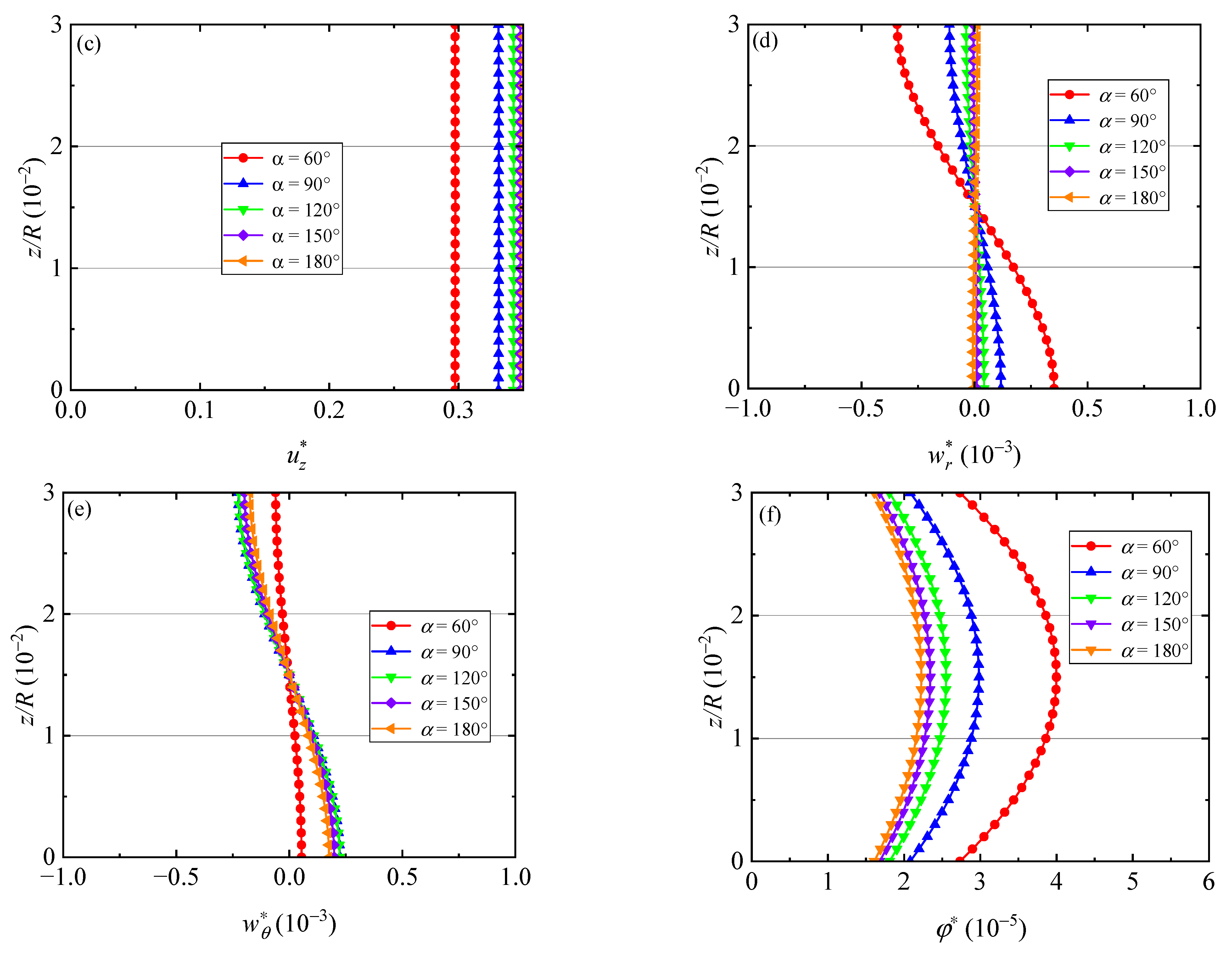
5.1. Effect of Different Angle Spans

We first examine the influence of different angular spans (α = 60°, 90°, 120°, 150°, 180°) on the free vibration characteristics of QC1/QC1/QC1 sector plates with SSSS boundary conditions. The interface compliance of the QC sector plate is set as K* = 0 (for the perfect interface case).

Table 2. First nine dimensionless frequencies Ω of the QC sector plate with different angle spans.

	Mode 1	Mode 2	Mode 3	Mode 4	Mode 5	Mode 6	Mode 7	Mode 8	Mode 9
60°	0.25155	0.55443	1.02786	1.67456	2.45837	2.48360	3.06823	3.47521	3.78644
90°	0.16669	0.46087	0.93422	1.58251	1.69499	2.12678	2.39382	3.00043	3.08747
120°	0.13666	0.42830	0.90155	1.34053	1.55034	1.65306	2.36242	2.52675	2.78594
150°	0.12279	0.41327	0.88645	1.15013	1.37255	1.53545	2.26953	2.34788	2.63863
180°	0.11528	0.40512	0.87826	1.03778	1.19043	1.52736	2.11632	2.33999	2.55534

shows the first nine dimensionless frequencies Ω of the QC sector plate with different angle spans. It can be seen from the table that with increasing α, the dimensionless frequencies Ω decrease, which indicates that the variation of α changes the stiffness of laminated sector plates and leads to a change in structural stability.

Figure 2 shows the variation of the phonon and phason displacements and the electric potential of the QC sector plate along the thickness direction at the first dimensionless frequency for the five different angular spans. It is observed that $u_r^{\ast }$ (Figure 2a) is insensitive with varying α and it is antisymmetric with respect to the midplane. The closer to the top and bottom surfaces, the greater the absolute value of $u_r^{\ast }$. $u_{\theta }^{\ast }$, $u_z^{\ast }$, $w_r^{\ast }$, $w_{\theta }^{\ast }$, and ${\phi }^{\ast }$ (Figure 2b–f) is. Also, $u_{\theta }^{\ast }$ is antisymmetric with respect to the midplane, with its absolute value at the top and bottom of the plate decreasing with increasing α. $u_z^{\ast }$ does not change with thickness, but changes with α, indicating again that a decrease in the angular span results in an increase in the stiffness of the QC plate. The absolute value of $w_r^{\ast }$ along the z-direction decreases with increasing α, and the absolute value of $w_{\theta }^{\ast }$ also increases with increasing α. The variation of ${\phi }^{\ast }$ becomes less evident as α changes, indicating a decrease in electric potential energy due to free vibration.

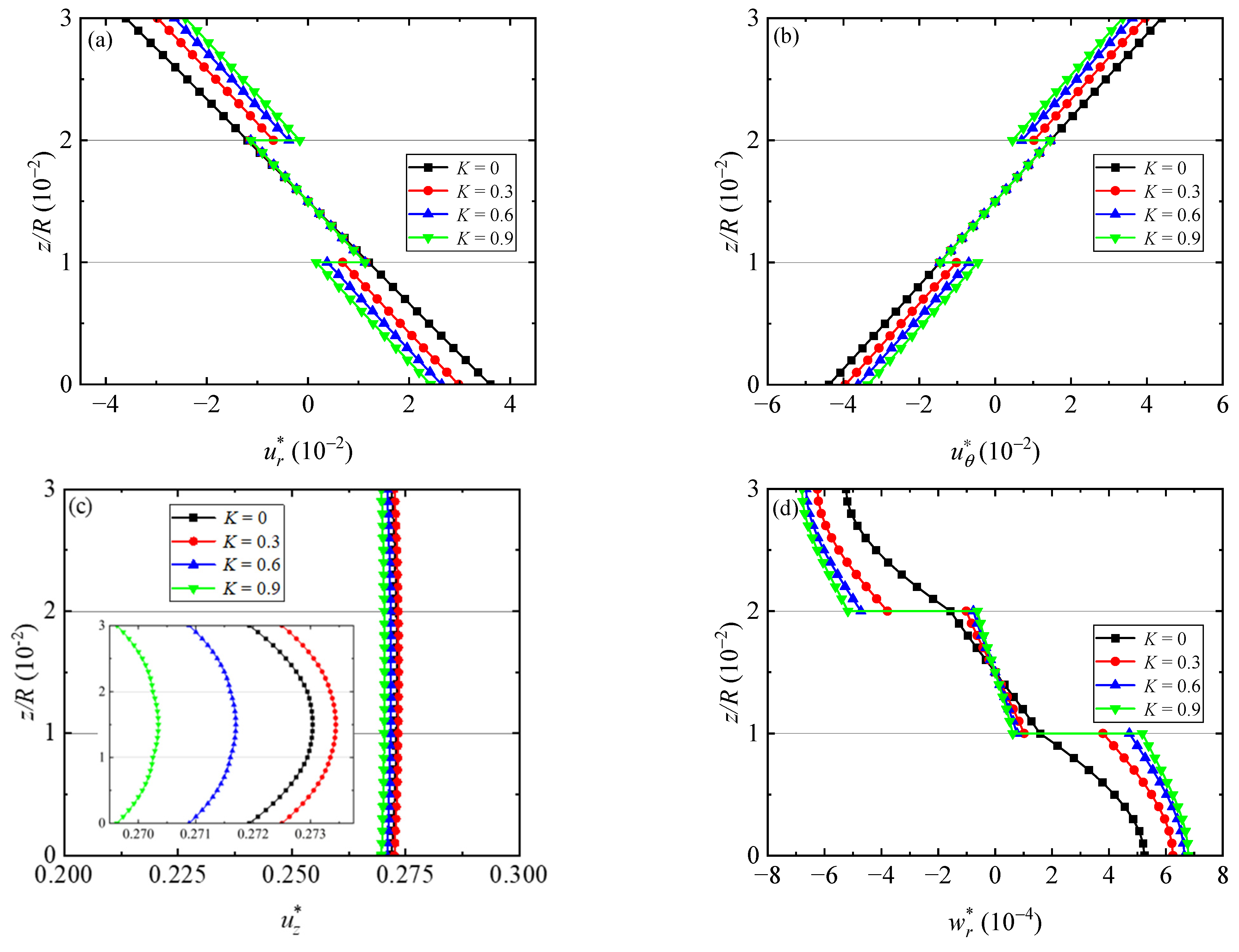
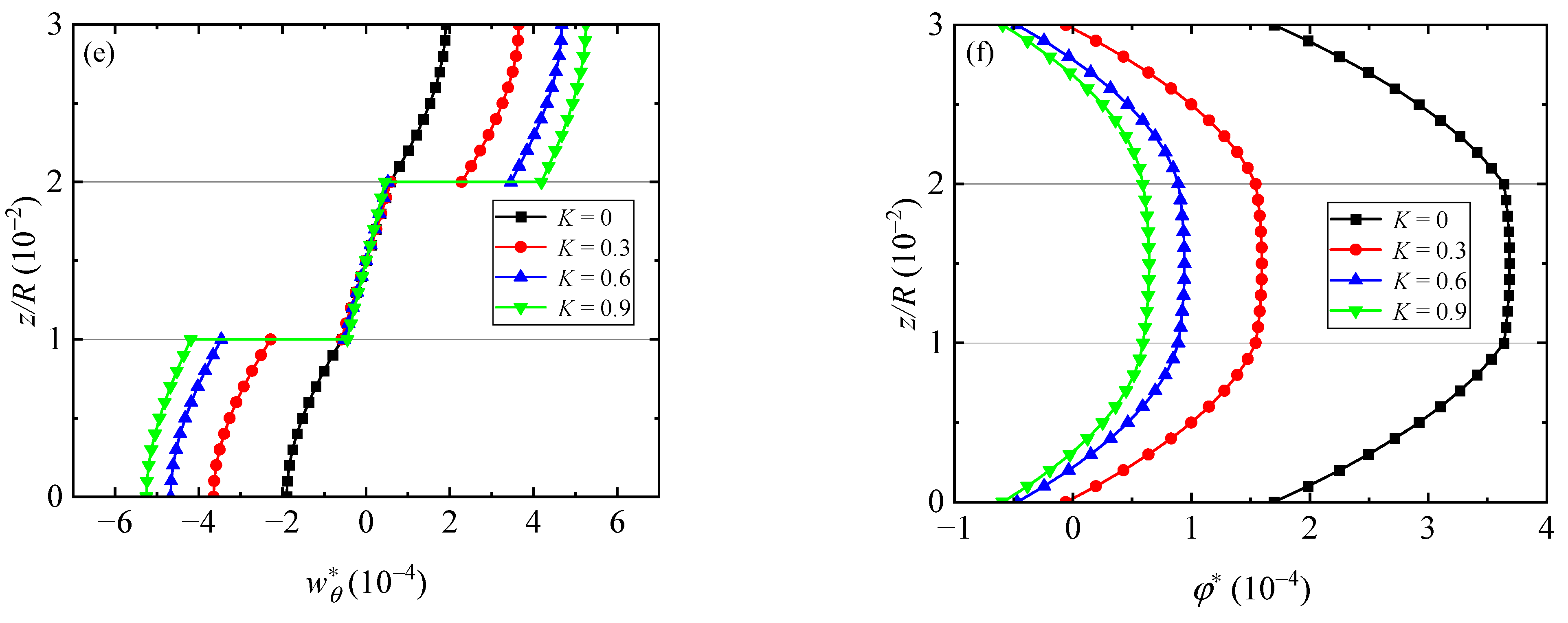
5.2. Effect of Different Interface Compliances

In this subsection, the influence of the interface compliance K* on the free vibration characteristics of QC sector plates with SCSC and zero electric potential boundary conditions is investigated. To simplify the model, we assume that (G₁)₃₃ = (G₁)₃₄ = (G₁)₄₃ = (G₁)₄₄ = 0, while other interface compliances are defined as (G₁)₁₁ = (G₁)₂₂ = (G₂)₅₅ = K* = 0, 0.3, 0.6, 0.9. In addition, the angular span of the QC sector plate is fixed at α = 30°.

Table 3. First nine dimensionless frequencies Ω of the QC sector plate with a dielectrically weakly conducting interface.

	Mode 1	Mode 2	Mode 3	Mode 4	Mode 5	Mode 6	Mode 7	Mode 8	Mode 9
K* = 0	0.83093	1.62415	2.70589	4.06200	5.48448	5.66161	5.67968	6.74528	7.11564
K* = 0.3	0.74856	1.36473	2.12847	3.01609	4.00536	5.17402	5.46680	5.66087	6.30747
K* = 0.6	0.69391	1.22516	1.87138	2.62394	3.47311	4.50307	5.44953	5.52350	5.64239
K* = 0.9	0.65336	1.13344	1.71800	2.40713	3.19707	4.17784	5.16437	5.43269	5.62441

shows the first nine dimensionless frequencies of the free vibration of the QC2/QC1/QC2 sector plate with a dielectrically weakly conducting interface. It can be seen from Table 3 that K* has a significant effect on the eigenfrequency Ω. In the same mode, Ω decreases with increasing K*. Since increasing the interface compliance will reduce the stiffness and strength of the laminated QC sector plate, this could cause fatigue damage in the structure. Furthermore, a weakly conducting interface also influences the dimensionless frequency of the QC sector plate.

Figure 3 shows the variation of the phonon and phason displacements and the electric potential of the QC sector plate along the thickness direction at the first dimensionless frequency with different interface compliances when the interface is weakly conducting. It is noted from this figure that when K* = 0, which corresponds to the perfect interface case, the displacements and electric potential are continuous between layers. If K* ≠ 0, $u_r^{\ast }$, $u_{\theta }^{\ast }$, $w_r^{\ast }$, $w_{\theta }^{\ast }$, and ${\phi }^{\ast }$ become discontinuous between the layers. It is observed that the variation trends of $u_r^{\ast }$ and $u_{\theta }^{\ast }$ (Figure 3a,b) for different K* are opposite to each other, but they are both antisymmetric with respect to z/R = 0.

Table 4. First nine dimensionless frequencies Ω of the QC sector plate with a dielectrically highly conducting interface.

	Mode 1	Mode 2	Mode 3	Mode 4	Mode 5	Mode 6	Mode 7	Mode 8	Mode 9
K* = 0	0.83093	1.62415	2.70589	4.06200	5.48448	5.66161	5.67968	6.74528	7.11564
K* = 0.3	0.74782	1.36231	2.12296	3.00605	3.98948	5.15054	5.46678	5.66055	6.27623
K* = 0.6	0.69318	1.22307	1.86704	2.61649	3.46174	4.48616	5.44951	5.50065	5.64205
K* = 0.9	0.65270	1.13167	1.71449	2.40124	3.18810	4.16407	5.14512	5.43267	5.62406

shows the first nine dimensionless frequencies of the free vibration of QC2/QC1/QC2 sector plates when the interface is highly conducting. It can be seen from this table that interface compliance has a significant effect on each eigenfrequency Ω. For the frequency on the same mode, Ω decreases with increasing K*.

Figure 4 shows the variation of the phonon and phason displacements and the electric potential of the QC sector plate along the thickness direction at the first dimensionless frequency for different interface compliances when the interface is highly conducting. The variation trends $u_r^{\ast }$ and $u_{\theta }^{\ast }$ (Figure 4a,b) are opposite to each other for varying K*, and they are antisymmetric with respect to z/R = 0. Displacements and electric potential are continuous if K* = 0. $u_z^{\ast }$ (Figure 4c) is nearly constant along the plate thickness for different K*, varying slightly around 0.27. It can be seen from Figure 4d,e that $w_r^{\ast }$ and $w_{\theta }^{\ast }$ are antisymmetric with respect to the midplane, and the vibration mode shape changes with changing K*. The electric potential is continuous under the condition of the highly conducting interface, which is different from Figure 4f.

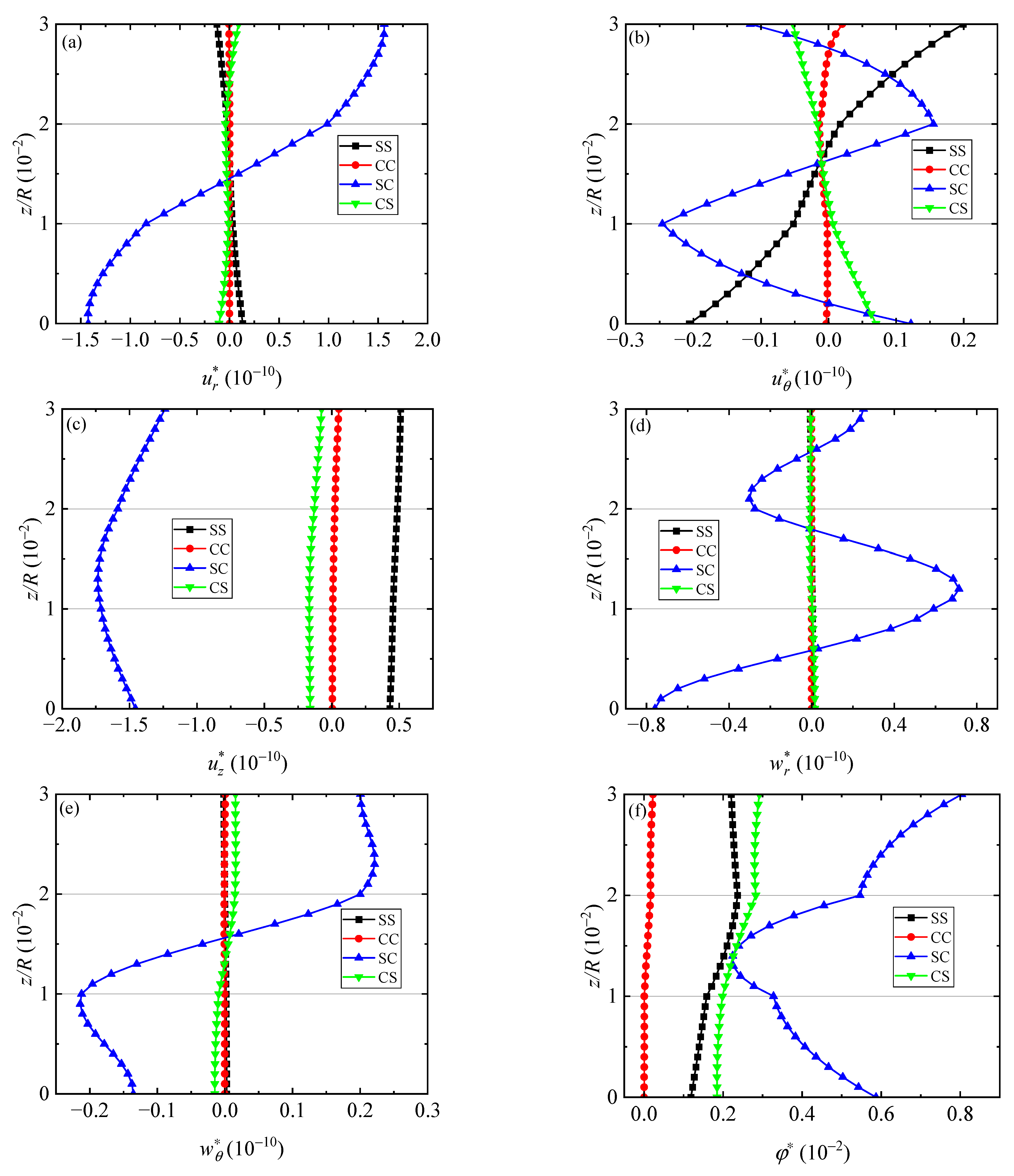
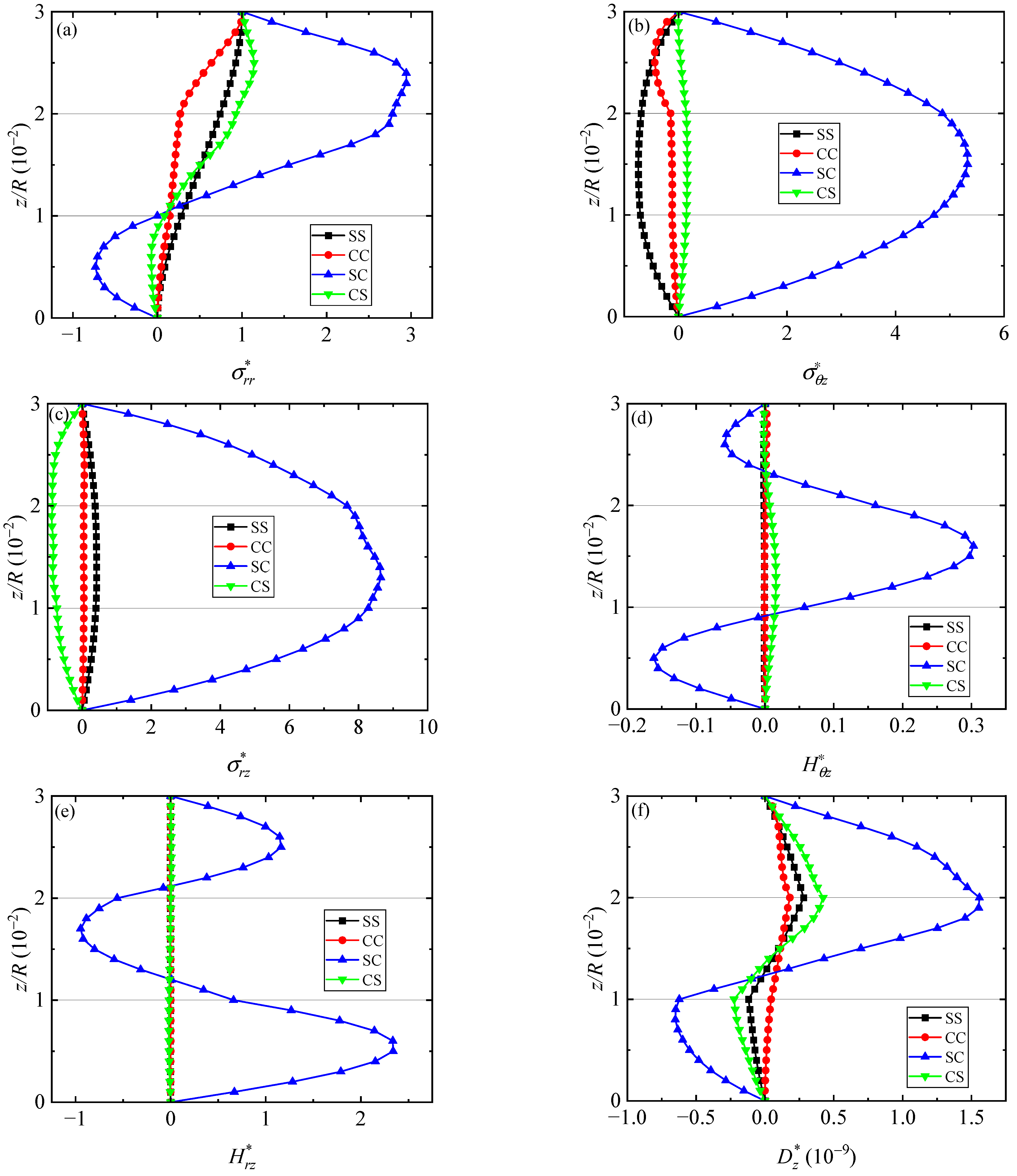
5.3. Effect of Different Boundary Conditions

In this subsection, we study the influence of four different boundary conditions on the modes of QC1/QC2/QC1 sector plates with perfect interfaces under the action of uniformly distributed mechanical excitation on the top surface. Other parameters of the QC sector plate are fixed as α = 60° and K* = 0. In Equation (26), the dimensionless external excitation frequency is fixed at ${\sigma }_0 = 1$, which is greater than its first dimensionless eigenfrequency as listed in Table 4.

Figure 5 shows the variation of the phonon and phason displacements and electric potential along the thickness direction under four different boundary conditions on the sides for θ = 0 and θ = α (with boundary conditions on the radial sides being fixed as SS): SS, CC, SC, and CS. According to Figure 5, the influence of simply supported and clamped boundary conditions on field variables is different. In Figure 5a, under the SC boundary, the closer to the top and bottom surfaces, the greater the amplitude of $u_r^{\ast }$ is, while there is nearly no change under the other three boundary conditions. In Figure 5b, the clamped boundary reduces the amplitude of $u_{\theta }^{\ast }$, and the amplitude under the CC boundary is almost zero. In Figure 5c, $u_z^{\ast }$ is nearly constant along the thickness direction, and its amplitude under the CC boundary condition is nearly zero. In Figure 5d,e, the SC boundary condition has the greatest influence on the amplitude of $w_r^{\ast }$ and $w_{\theta }^{\ast }$, and the amplitude of phason displacements under other boundary conditions is almost zero. In Figure 5f, the electric potential is also mostly affected by the SC boundary condition with its amplitude being the largest in the midplane, while its amplitude under the other boundary conditions is very small (especially for the CC, it is zero).

Figure 6 shows the variation of the phonon and phason stresses and electric displacements along the thickness direction under the four different lateral boundary conditions. The modes of stresses and electric displacements are zero on the top and bottom surfaces of the sector plate, which meets the assumption that the traction and electric displacements on the top and bottom surfaces are zero. It is observed from Figure 6 that among all boundary conditions, the influence of simply supported and clamped boundary conditions on field variables is completely different, with the SC boundary having the greatest influence on the change in field variables along the thickness direction. The amplitude of stresses and electric displacements under SS, CC, and CS boundaries change slightly (with the amplitude of the CC case being the closest to zero). The stresses and electric displacements caused by forced vibration under the SC boundary change most obviously and they further fluctuate as sinusoidal curves. In Figure 6a,d–f, the amplitude reaches the extreme value at the interface, and in Figure 6b,c, the amplitude reaches the maximum value in the midplane.

6. Summary

In this paper, the dynamic response of a layered 2D PQC sector plate with an arbitrary angular span is studied using a semi-analytical method. The state equations of a 2D PQC sector plate are obtained by using the state-space method based on the QC linear elasticity. The DQM and Fourier series expansions are used to satisfy the simply supported and clamped boundary conditions. The propagator matrix method is used to combine the ordinary differential form equations with the interface matrix to obtain the solutions of all field variables. The semi-analytical method proposed in this study is suitable for analyzing the vibration of 3D plates with arbitrary layers and sectorial shapes, which includes the special case of a layered rectangle. In the numerical examples, the effects of different angular spans, different interface compliances, and different lateral boundary conditions on the dimensionless frequencies and field variables distribution of QC sector plates are discussed. The main conclusions are listed as follows:

• The variation of the sector angle α changes the stiffness of laminated QC sector plates, and consequently, it results in different modes for different α;
• An increase in interface compliance will reduce the stiffness and strength of the laminated QC sector plate, and the displacements in the r- and θ-directions (in addition to $u_z^{\ast }$) are discontinuous from one layer to the other due to the interface imperfection;
• Out of all the boundary conditions, the impacts of simply supported and clamped boundary conditions on field variables are notably distinct. The mixed case where one side is simply supported and the other is clamped has the most significant effect on the amplitude variation of field variables along the thickness direction.

References

1. Shechtman, D.; Blech, I.; Gratias, D.; Cahn, J.W. Metallic phase with long-range orientational order and no translational symmetry. Phys. Rev. Lett. 1984, 53, 1951–1953. [Google Scholar] [CrossRef]
2. Fan, T.Y.; Guo, Y.C. Mathematical methods for a class of mixed boundary-value problems of planar pentagonal quasicrystal and some solutions. Sci. China Ser. A-Math. 1997, 40, 990–1003. [Google Scholar] [CrossRef]
3. Fan, T.Y. Mathematical theory and methods of mechanics of quasicrystalline materials. Engineering 2013, 5, 407–448. [Google Scholar] [CrossRef]
4. Bohra, M.; Pavan, T.M.; Fournee, V.; Mandal, R.K. Growth, structure and thermal stability of quasicrystalline Al-Pd-Mn-Ga thin films. Appl. Surf. Sci. 2020, 505, 4. [Google Scholar] [CrossRef]
5. Shi, N.C.; Min, L.Q.; Shen, B.M. The configuration of quasi-crystal unit-cell and deduction of quasi-lattice. Sci. China Ser. B-Chem. 1992, 35, 735–744. [Google Scholar]
6. Dubois, J.M. Properties- and applications of quasicrystals and complex metallic alloys. Chem. Soc. Rev. 2012, 41, 6760–6777. [Google Scholar] [CrossRef]
7. Fujiwara, T.; Ishii, Y. Introduction to quasicrystals. In Quasicrystals; Fujiwara, T., Ishii, Y., Eds.; Elsevier Science Bv: Amsterdam, The Netherlands, 2008; pp. 1–9. [Google Scholar]
8. Bak, P. Phenomenological theory of icosahedral incommensurate (quasiperiodic) order in Mn-Al alloys. Phys. Rev. Lett. 1985, 54, 1517–1519. [Google Scholar] [CrossRef]
9. Lubensky, T.C.; Ramaswamy, S.; Toner, J. Dislocation motion in quasicrystals and implication for macroscopic properties. Phys. Rev. B 1986, 33, 7715–7719. [Google Scholar] [CrossRef] [PubMed]
10. Lubensky, T.; Ramaswamy, S.; Toner, J. Hydrodynamics of icosahedral quasicrystals. Phys. Rev. B 1985, 32, 7444. [Google Scholar] [CrossRef]
11. Bak, P. Symmetry, stability, and elastic properties of icosahedral incommensurate crystals. Phys. Rev. B 1985, 32, 5764. [Google Scholar] [CrossRef]
12. Ding, D.H.; Yang, W.G.; Hu, C.Z.; Wang, R. Generalized elasticity theory of quasicrystals. Phys. Rev. B 1993, 48, 7003–7010. [Google Scholar] [CrossRef] [PubMed]
13. Agiasofitou, E.; Lazar, M. On the equations of motion of dislocations in quasicrystals. Mech. Res. Commun. 2014, 57, 27–33. [Google Scholar] [CrossRef]
14. Fan, T.; Wang, X.; Li, W.; Zhu, A.Y. Elasto-hydrodynamics of quasicrystals. Philos. Mag. 2009, 89, 501–512. [Google Scholar] [CrossRef]
15. Rochal, S.; Lorman, V. Anisotropy of acoustic-phonon properties of an icosahedral quasicrystal at high temperature due to phonon-phason coupling. Phys. Rev. B 2000, 62, 874. [Google Scholar] [CrossRef]
16. Rochal, S.; Lorman, V. Minimal model of the phonon-phason dynamics in icosahedral quasicrystals and its application to the problem of internal friction in the i-AlPdMn alloy. Phys. Rev. B 2002, 66, 144204. [Google Scholar] [CrossRef]
17. Agiasofitou, E.; Lazar, M. The elastodynamic model of wave-telegraph type for quasicrystals. Int. J. Solids Struct. 2014, 51, 923–929. [Google Scholar] [CrossRef]
18. Ferreira, T.; De Oliveira, I.L.; Zepon, G.; Bolfarini, C. Rotational outward solidification casting: An innovative single-step process to produce a functionally graded aluminum reinforced with quasicrystal approximant phases. Mater. Des. 2020, 189, 10. [Google Scholar] [CrossRef]
19. Li, L.H.; Yun, G.H. Elastic fields around a nanosized elliptic hole in decagonal quasicrystals. Chin. Phys. B 2014, 23, 5. [Google Scholar] [CrossRef]
20. Pan, E.; Heyliger, P.R. Free vibrations of simply supported and multilayered magneto-electro-elastic plates. J. Sound Vib. 2002, 252, 429–442. [Google Scholar] [CrossRef]
21. Yang, L.Z.; Gao, Y.; Pan, E.; Waksmanski, N. An exact solution for a multilayered two-dimensional decagonal quasicrystal plate. Int. J. Solids Struct. 2014, 51, 1737–1749. [Google Scholar] [CrossRef]
22. Guo, J.H.; Liu, G.T. Analytic solutions to problem of elliptic hole with two straight cracks in one-dimensional hexagonal quasicrystals. Appl. Math. Mech. -Engl. Ed. 2008, 29, 485–493. [Google Scholar] [CrossRef]
23. Guo, J.H.; Zhang, M.; Chen, W.Q.; Zhang, X. Free and forced vibration of layered one-dimensional quasicrystal nanoplates with modified couple-stress effect. Sci. China (Phys. Mech. Astron.) 2020, 63, 124–125. [Google Scholar] [CrossRef]
24. Zhang, L.; Guo, J.H.; Xing, Y.M. Bending deformation of multilayered one-dimensional hexagonal piezoelectric quasicrystal nanoplates with nonlocal effect. Int. J. Solids Struct. 2018, 132, 278–302. [Google Scholar] [CrossRef]
25. Huang, Y.Z.; Li, Y.; Zhang, L.L.; Zhang, H.; Gao, Y. Dynamic analysis of a multilayered piezoelectric two-dimensional quasicrystal cylindrical shell filled with compressible fluid using the state-space approach. Acta Mech. 2020, 231, 2351–2368. [Google Scholar] [CrossRef]
26. Li, X.F. Elastohydrodynamic problems in quasicrystal elasticity theory and wave propagation. Philos. Mag. 2013, 93, 1500–1519. [Google Scholar] [CrossRef]
27. Pan, E.; Han, F. Exact solution for functionally graded and layered magneto-electro-elastic plates. Int. J. Eng. Sci. 2005, 43, 321–339. [Google Scholar] [CrossRef]
28. Guo, J.H.; Chen, J.Y.; Pan, E. A three-dimensional size-dependent layered model for simply-supported and functionally graded magnetoelectroelastic plates. Acta Mech. Solida Sin. 2018, 31, 652–671. [Google Scholar] [CrossRef]
29. Lu, C.F.; Lim, C.W.; Chen, W.Q. Exact solutions for free vibrations of functionally graded thick plates on elastic foundations. Mech. Adv. Mater. Struct. 2009, 16, 576–584. [Google Scholar] [CrossRef]
30. Ying, J.; Lu, C.F.; Lim, C.W. 3D thermoelasticity solutions for functionally graded thick plates. J. Zhejiang Univ.-Sci. A 2009, 10, 327–336. [Google Scholar] [CrossRef]
31. Striz, A.G.; Wang, X.; Bert, C.W. Harmonic differential quadrature method and applications to analysis of structural components. Acta Mech. 1995, 111, 85–94. [Google Scholar] [CrossRef]
32. Chen, W.Q.; Lv, C.F.; Bian, Z.G. Free vibration analysis of generally laminated beams via state-space-based differential quadrature. Compos. Struct. 2004, 63, 417–425. [Google Scholar] [CrossRef]
33. Lü, C.F.; Chen, W.Q.; Shao, J.W. Semi-analytical three-dimensional elasticity solutions for generally laminated composite plates. Eur. J. Mech.- A/Solids 2008, 27, 899–917. [Google Scholar] [CrossRef]
34. Zhou, Y.Y.; Chen, W.Q.; Lü, C.F. Semi-analytical solution for orthotropic piezoelectric laminates in cylindrical bending with interfacial imperfections. Compos. Struct. 2010, 92, 1009–1018. [Google Scholar] [CrossRef]
35. Bert, C.W.; Malik, M. Differential quadrature: A powerful new technique for analysis of composite structures. Compos. Struct. 1997, 39, 179–189. [Google Scholar] [CrossRef]
36. Wang, X.; Bert, C.W.; Striz, A.G. Differential quadrature analysis of deflection, buckling, and free-vibration of beams and rectangular plates. Comput. Struct. 1993, 48, 473–479. [Google Scholar] [CrossRef]
37. Alibeigloo, A.; Kani, A.M. 3D free vibration analysis of laminated cylindrical shell integrated piezoelectric layers using the differential quadrature method. Appl. Math. Model. 2010, 34, 4123–4137. [Google Scholar] [CrossRef]
38. Jang, S.K.; Bert, C.W. Free-vibration of stepped beams—Exact and numerical-solutions. J. Sound Vib. 1989, 130, 342–346. [Google Scholar] [CrossRef]
39. Feng, X.; Fan, X.Y.; Li, Y.; Zhang, H.; Zhang, L.; Gao, Y. Static response and free vibration analysis for cubic quasicrystal laminates with imperfect interfaces. Eur. J. Mech.-A/Solids 2021, 90, 104365. [Google Scholar] [CrossRef]
40. Botta, F.; Cerri, G. Wave propagation in Reissner-Mindlin piezoelectric coupled cylinder with non-constant electric field through the thickness. Int. J. Solids Struct. 2007, 44, 6201–6219. [Google Scholar] [CrossRef]
41. Huang, B.; Kim, H.S. Free-edge interlaminar stress analysis of piezo-bonded composite laminates under symmetric electric excitation. Int. J. Solids Struct. 2014, 51, 1246–1252. [Google Scholar] [CrossRef]
42. Khalid, S.; Lee, J.; Kim, H.S. Series solution-based approach for the interlaminar stress analysis of smart composites under thermo-electro-mechanical loading. Mathematics 2022, 10, 15. [Google Scholar] [CrossRef]
43. Li, X.Y.; Li, P.D.; Wu, T.H.; Shi, M.X.; Zhu, Z. Three-dimensional fundamental solutions for one-dimensional hexagonal quasicrystal with piezoelectric effect. Phys. Lett. A 2014, 378, 826–834. [Google Scholar] [CrossRef]
44. Chen, T.Y. Thermal conduction of a circular inclusion with variable interface parameter. Int. J. Solids Struct. 2001, 38, 3081–3097. [Google Scholar] [CrossRef]
45. Fan, H.; Sze, K.Y. A micro-mechanics model for imperfect interface in dielectric materials. Mech. Mater. 2001, 33, 363–370. [Google Scholar] [CrossRef]
46. Wang, X.; Pan, E. A moving screw dislocation interacting with an imperfect piezoelectric bimaterial interface. Phys. Status Solidi B-Basic Solid State Phys. 2007, 244, 1940–1956. [Google Scholar] [CrossRef]
47. Fan, H.; Wang, G.F. Screw dislocation interacting with imperfect interface. Mech. Mater. 2003, 35, 943–953. [Google Scholar] [CrossRef]
48. Wang, X.; Zhong, Z. Three-dimensional solution of smart laminated anisotropic circular cylindrical shells with imperfect bonding. Int. J. Solids Struct. 2003, 40, 5901–5921. [Google Scholar] [CrossRef]
49. Benveniste, Y. A general interface model for a three-dimensional curved thin anisotropic interphase between two anisotropic media. J. Mech. Phys. Solids 2006, 54, 708–734. [Google Scholar] [CrossRef]
50. Wang, X.; Pan, E.; Roy, A.K. New phenomena concerning a screw dislocation interacting with two imperfect interfaces. J. Mech. Phys. Solids 2007, 55, 2717–2734. [Google Scholar] [CrossRef]
51. Kattis, M.A.; Mavroyannis, G. Feeble interfaces in bimaterials. Acta Mech. 2006, 185, 11–29. [Google Scholar] [CrossRef]
52. Wang, X.; Pan, E. Exact solutions for simply supported and multilayered piezothermoelastic plates with imperfect interfaces. Open Mech. J. 2007, 1, 1–10. [Google Scholar] [CrossRef]
53. Chen, W.Q.; Cai, J.B.; Ye, G.R.; Wang, Y.F. Exact three-dimensional solutions of laminated orthotropic piezoelectric rectangular plates featuring interlaminar bonding imperfections modeled by a general spring layer. Int. J. Solids Struct. 2004, 41, 5247–5263. [Google Scholar] [CrossRef]
54. Hwu, C. Anisotropic Elastic Plates; Springer: New York, NY, USA, 2010; pp. 1–673. [Google Scholar]
55. Liu, C.; Feng, X.; Li, Y.; Zhang, L.; Gao, Y. Static solution of two-dimensional decagonal piezoelectric quasicrystal laminates with mixed boundary conditions. Mech. Adv. Mater. Struct. 2022, 1–17. [Google Scholar] [CrossRef]
Figure 1. The structure of a layered QC sector plate with imperfect interfaces.
Crystals 13 01412 g001
Figure 2. Variation of the phonon and phason displacements and electric potential along the thickness direction for different angular spans α: (a) u r , (b) u θ , (c) u z , (d) w r , (e) w θ , and (f) φ .
Crystals 13 01412 g002aCrystals 13 01412 g002b
Figure 3. Variation of the phonon and phason displacements and electric potential along the thickness direction for different interface compliances K* for the weakly conducting interface: (a) u r , (b) u θ , (c) u z , (d) w r , (e) w θ , and (f) φ .
Crystals 13 01412 g003
Figure 4. Variation of the phonon and phason displacements and electric potential along the thickness direction for different interface compliances K* for the highly conducting interface: (a) u r , (b) u θ , (c) u z , (d) w r , (e) w θ , and (f) φ .
Crystals 13 01412 g004aCrystals 13 01412 g004b
Figure 5. Variation of the phonon and phason displacements and electric potential along the thickness direction under four lateral boundary conditions: (a) u r , (b) u θ , (c) u z , (d) w r , (e) w θ , and (f) φ .
Crystals 13 01412 g005
Figure 6. Variation of the phonon and phason stresses and electric displacements along the thickness direction under four lateral boundary conditions: (a) σ z z , (b) σ θ z , (c) σ r z , (d) H θ z , (e) H r z , and (f) D z .
Crystals 13 01412 g006