
Comparison and Determination of Optimal Machine Learning Model for Predicting Generation of Coal Fly Ash


Abstract
:1. Introduction
2. Dataset
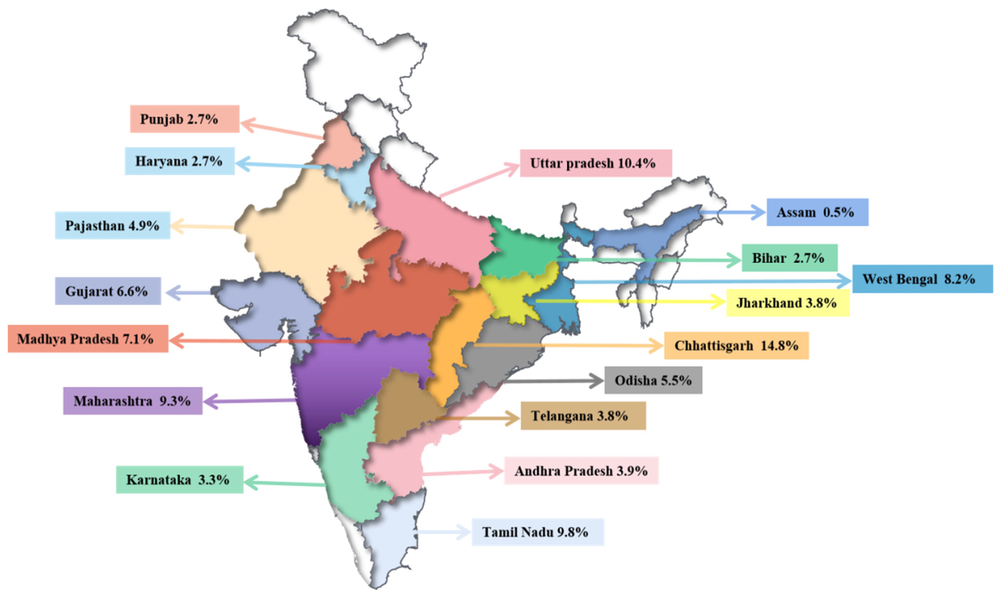
2.1. Data Collection
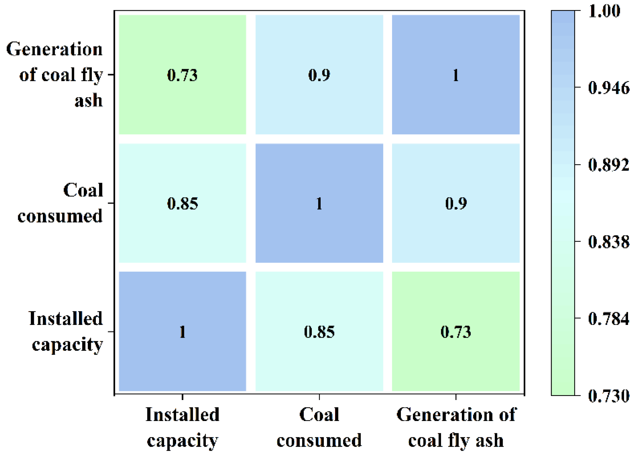
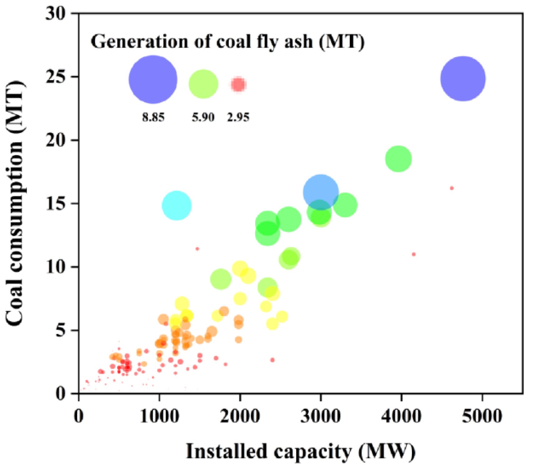
2.2. Data Analysis
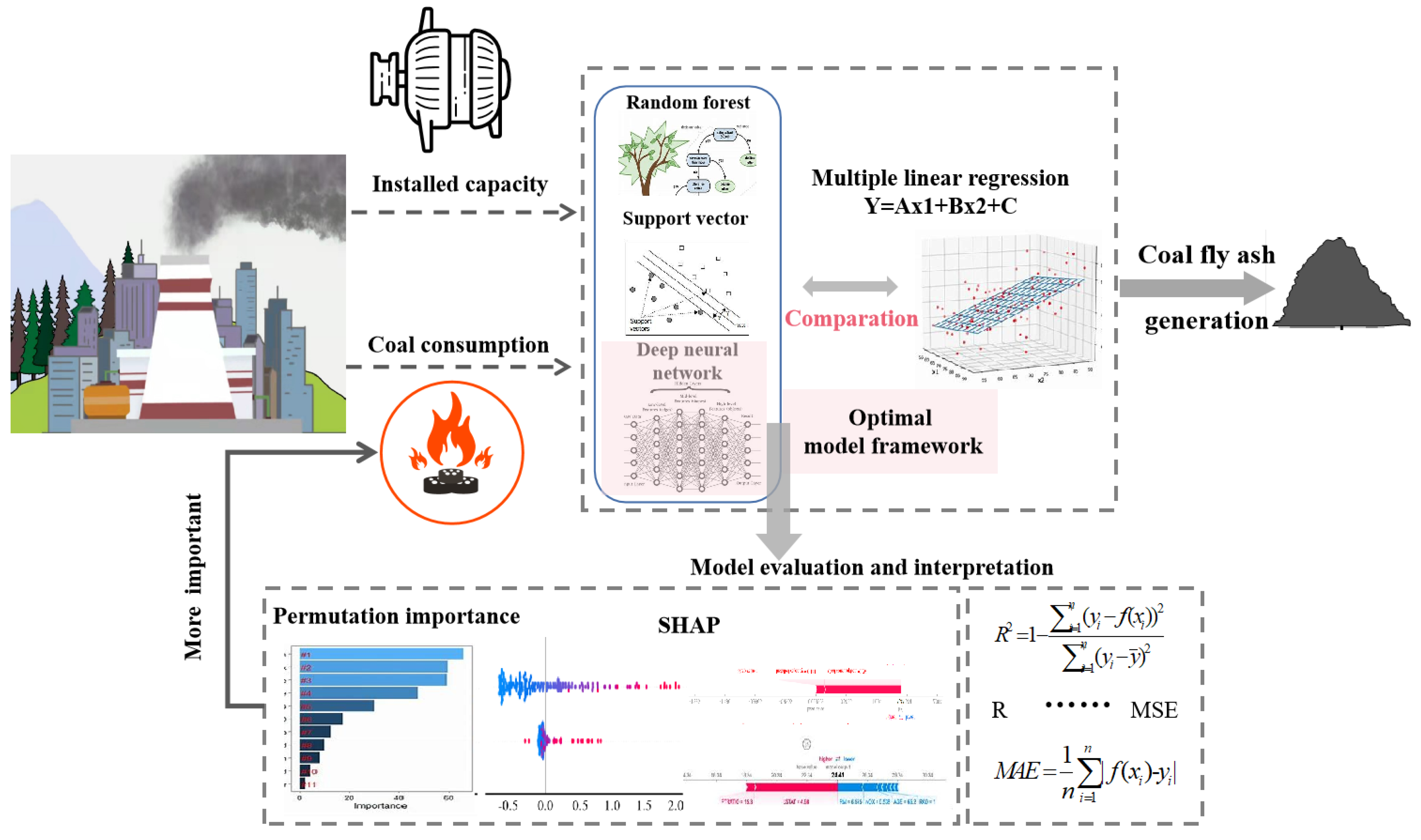
3. Methodology
3.1. Modeling Methods
3.1.1. Random Forest
- Random sampling and training decision tree: The original data population with sample size N is randomly sampled N times, and each time, the samples need to be put back [23]. N samples formed at last are used to train a decision tree;
- Randomly selected attributes as node-splitting attributes: When the nodes of the decision tree are split, m attributes (m << M) should be randomly selected from the M attributes of each sample, and then some strategies (such as information gain) should be adopted to select one attribute as the final split attribute of the node;
- Step 2 is repeated until the tree cannot be split, noting that no pruning occurs during the entire decision tree formation process;
- A large number of decision trees are established according to steps 1~3 to form an RF.
3.1.2. Support Vector Regression
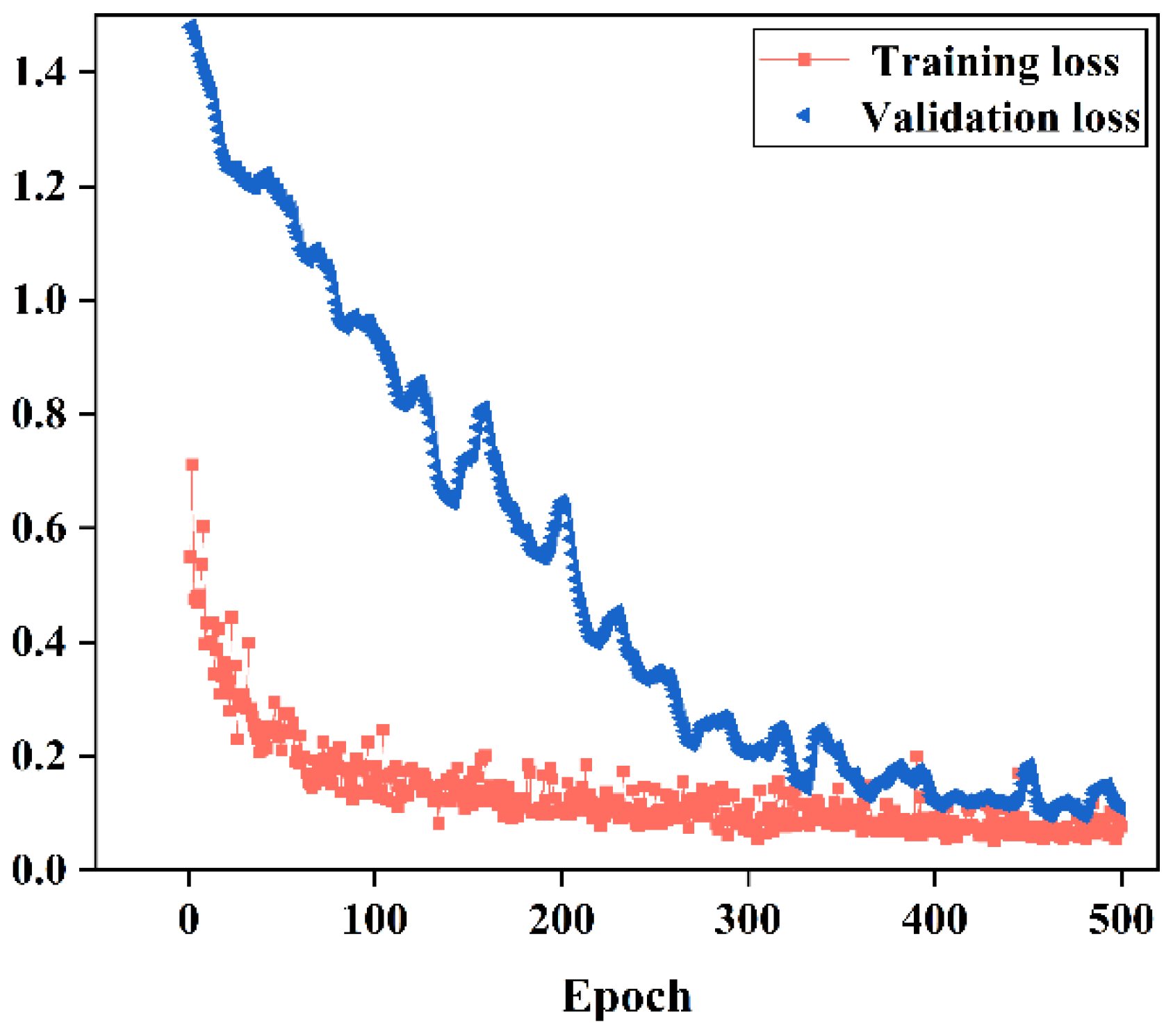
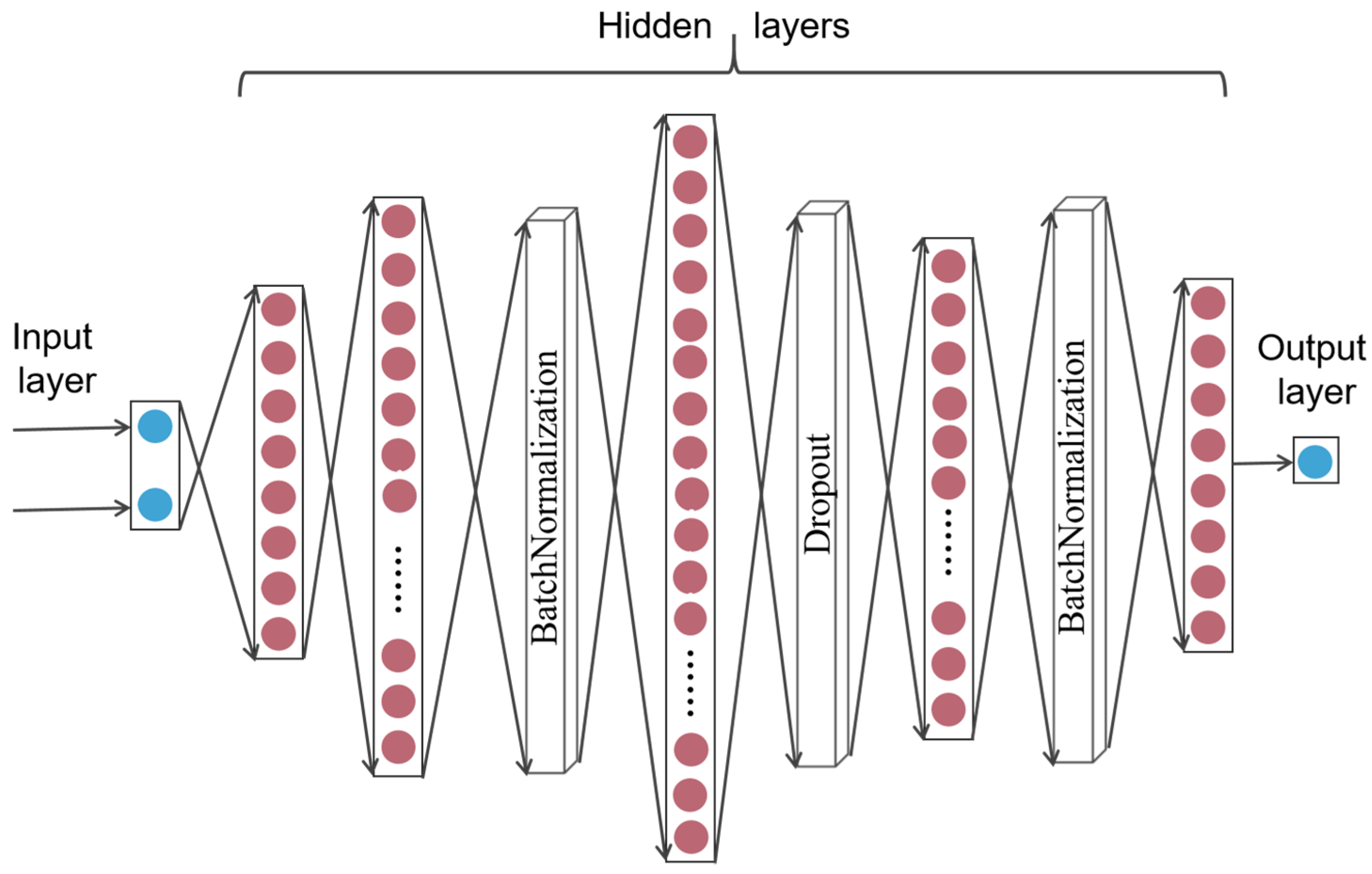
3.1.3. Deep Neural Network
3.2. Dataset Preprocessing and Splitting
3.3. Model Evaluation
4. Result and Discussion
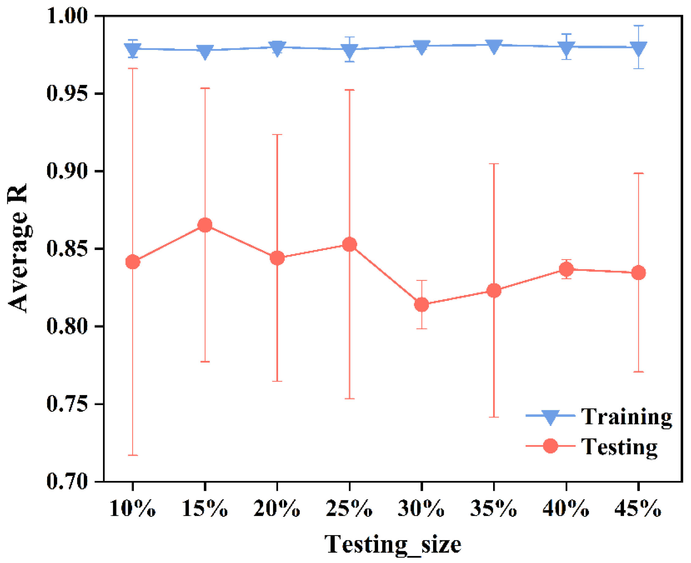
4.1. Determination of Dataset Division Ratio
4.2. Parameters of the Model
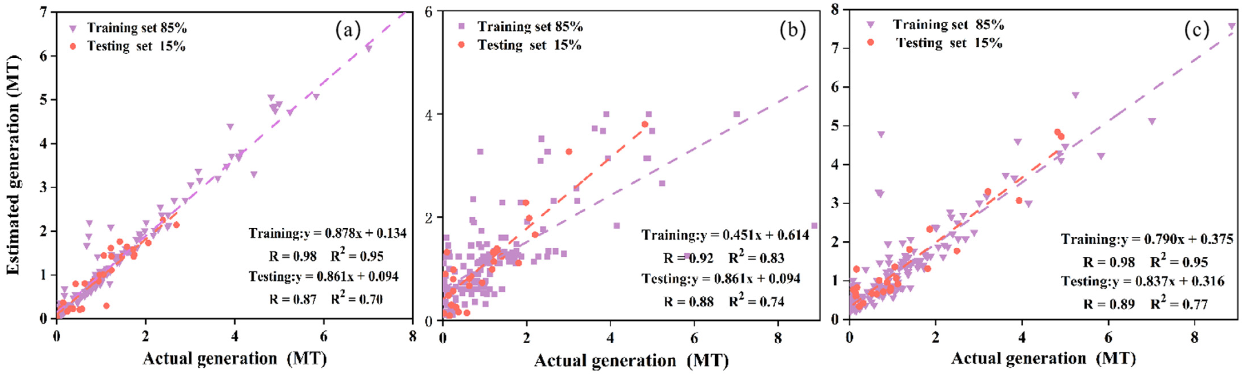
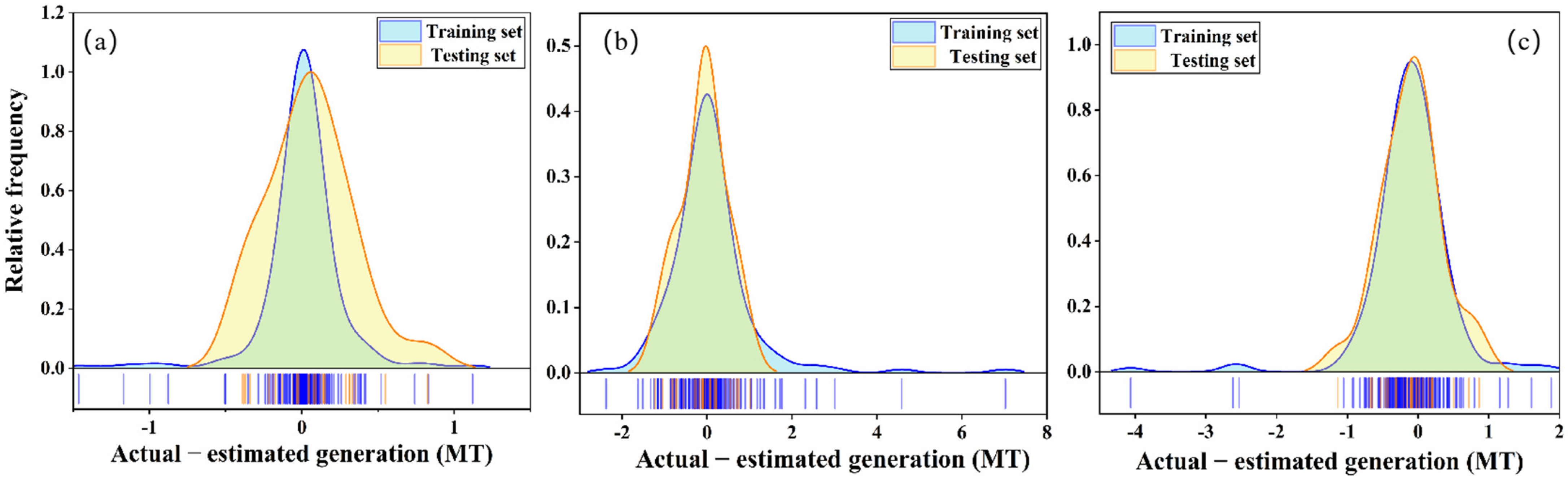
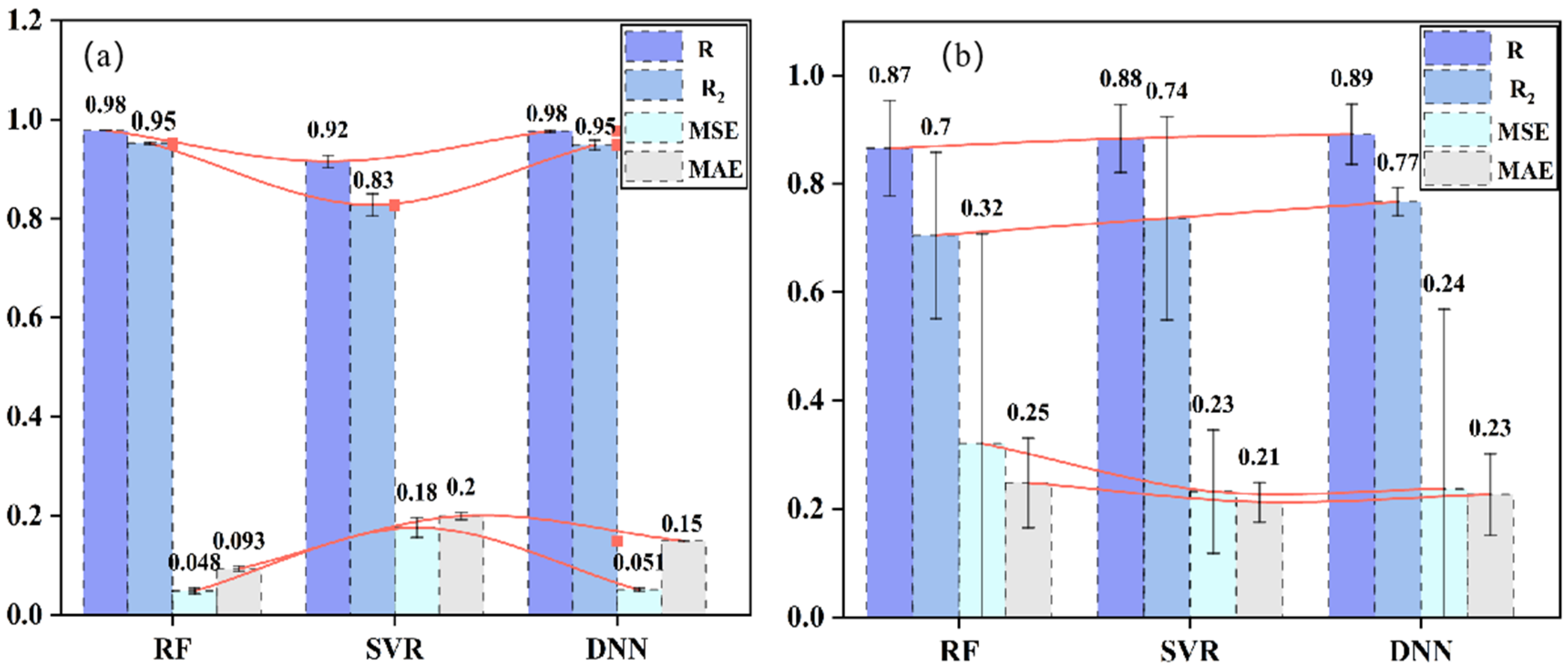
4.3. Comparative Analysis of Model Performance
4.4. Comparison with Multiple Linear Regression
4.5. Feature Analysis
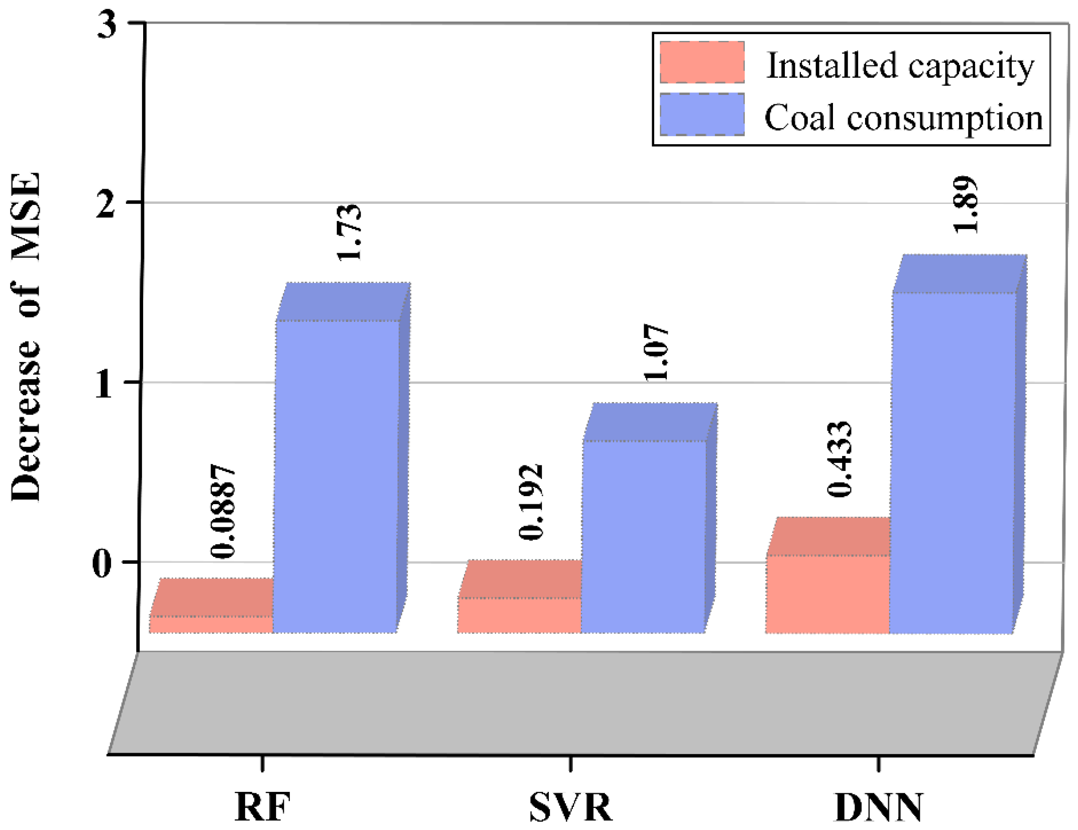
4.5.1. Permutation Importance
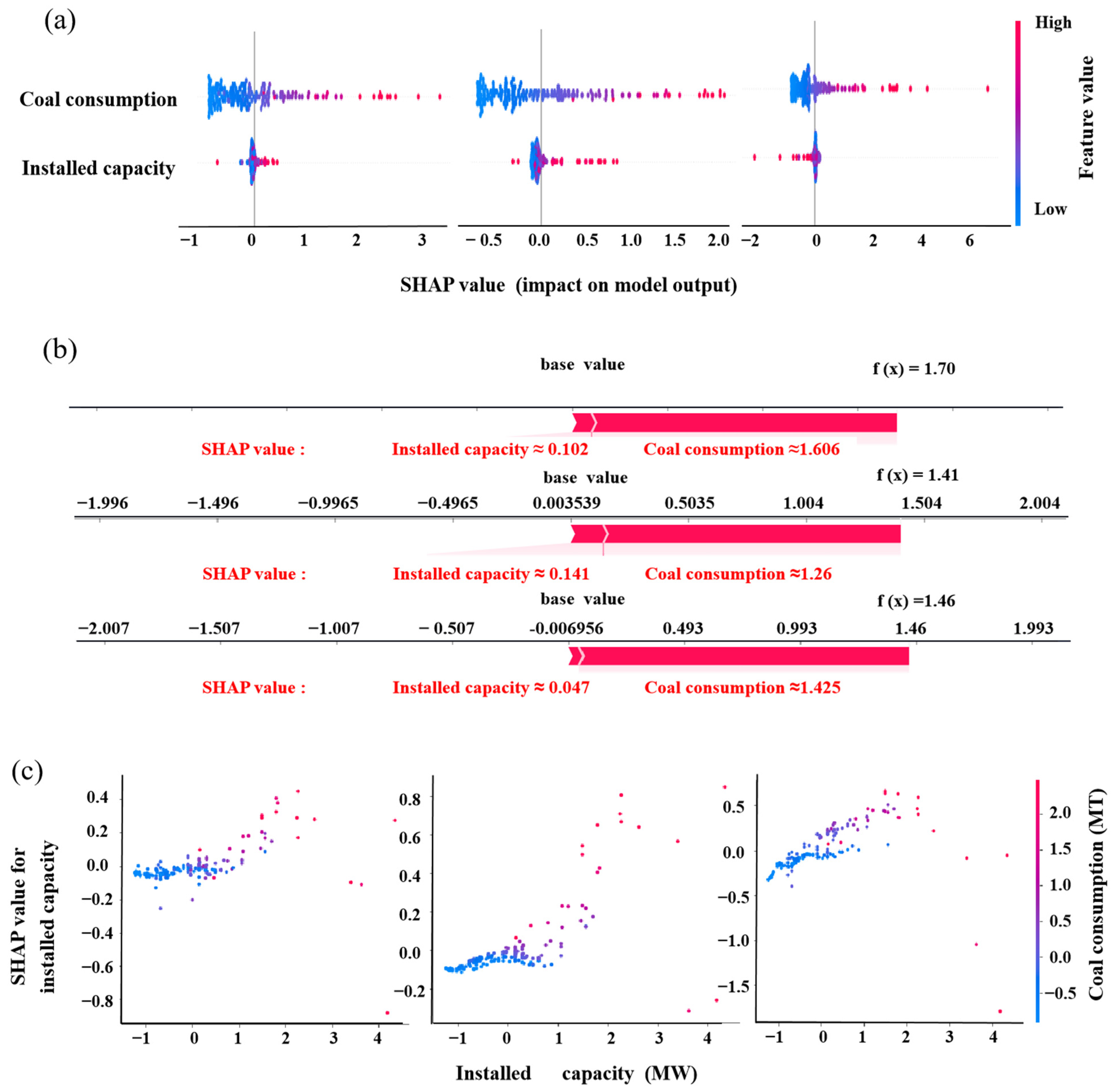
4.5.2. SHAP
5. Significance and Outlook
6. Conclusions
- (1)
- Among the three model algorithms, the DNN model had the best performance. R and R2 on the training set were 0.98 and 0.95, whereas these on the testing set were 0.89 and 0.77, respectively;
- (2)
- The R2 of the traditional multiple linear regression equation on the testing set was 0.76, higher than those of RF and SVR models, but lower than that of the DNN model;
- (3)
- Permutation importance and SHAP both indicated that coal consumption had a greater positive effect on the generation of CFA. As influenced by other factors, the influence of installed capacity on CFA generation was as significant as coal consumed and could be negative for some special data samples.
Author Contributions
Funding
Institutional Review Board Statement
Informed Consent Statement
Data Availability Statement
Acknowledgments
Conflicts of Interest
References
- Naqvi, S.Z.; Ramkumar, J.; Kar, K.K. Coal-based fly ash. In Handbook of Fly Ash; Kar, K.K., Ed.; Butterworth-Heinemann: Oxford, UK, 2022; pp. 3–33. [Google Scholar] [CrossRef]
- IEA. Electricity Market Report; IEA: Paris, France, 2022; Available online: https://www.iea.org/reports/electricity-market-report-january-2022 (accessed on 25 February 2022).
- IEA. Global Energy Review; IEA: Paris, France, 2021; Available online: https://www.iea.org/reports/global-energy-review-2021 (accessed on 25 February 2022).
- Wang, X.Y. Evaluation of the hydration heat and strength progress of cement-fly ash binary composite. J. Ceram. Process. Res. 2020, 21, 622–631. [Google Scholar] [CrossRef]
- Mathapati, M.; Amate, K.; Durga Prasad, C.; Jayavardhana, M.L.; Hemanth Raju, T. A review on fly ash utilization. Materials 2022, 50, 1535–1540. [Google Scholar] [CrossRef]
- Arora, S. An Ashen Legacy: India’s Thermal Power Ash Mismanagement; Centre for Science and Environment: New Delhi, India, 2020. [Google Scholar]
- Blaha, U.; Sapkota, B.; Appel, E.; Stanjek, H.; Rösler, W. Micro-scale grain-size analysis and magnetic properties of coal-fired power plant fly ash and its relevance for environmental magnetic pollution studies. Atmos. Environ. 2008, 42, 8359–8370. [Google Scholar] [CrossRef]
- Chowdhury, A.; Naz, A.; Chowdhury, A. Waste to resource: Applicability of fly ash as landfill geoliner to control ground water pollution. Materials 2021, 20, 897. [Google Scholar] [CrossRef]
- Chen, Q.; Chen, L.; Li, J.; Guo, Y.; Wang, Y.; Wei, W.; Liu, C.; Wu, J.; Tou, F.; Wang, X.; et al. Increasing mercury risk of fly ash generated from coal-fired power plants in China. J. Hazard. Mater. 2022, 429, 128296. [Google Scholar] [CrossRef]
- Jiang, A.; Zhao, J. Experimental Study of Desulfurized Fly Ash Used for Cement Admixture. In Proceedings of Civil Engineering in China–Current Practice and Research Report; Hindawi: Hebei, China, 2010; pp. 1038–1042. [Google Scholar]
- Ragipani, R.; Escobar, E.; Prentice, D.; Bustillos, S.; Simonetti, D.; Sant, G.; Wang, B. Selective sulfur removal from semi-dry flue gas desulfurization coal fly ash for concrete and carbon dioxide capture applications. Waste Manag. 2021, 121, 117–126. [Google Scholar] [CrossRef]
- Shanmugan, S.; Deepak, V.; Nagaraj, J.; Jangir, D.; Jegan, S.V.; Palani, S. Enhancing the use of coal-fly ash in coarse aggregates concrete. Mater. Today Proc. 2020, 30, 174–182. [Google Scholar] [CrossRef]
- Kotelnikova, A.D.; Rogova, O.B.; Karpukhina, E.A.; Solopov, A.B.; Levin, I.S.; Levkina, V.V.; Proskurnin, M.A.; Volkov, D.S. Assessment of the structure, composition, and agrochemical properties of fly ash and ash-and-slug waste from coal-fired power plants for their possible use as soil ameliorants. J. Clean. Prod. 2022, 333, 130088. [Google Scholar] [CrossRef]
- Zhu, M.; Ji, R.; Li, Z.; Wang, H.; Liu, L.; Zhang, Z. Preparation of glass ceramic foams for thermal insulation applications from coal fly ash and waste glass. Constr. Build. Mater. 2016, 112, 398–405. [Google Scholar] [CrossRef]
- Zahari, N.M.; Mohamad, D.; Arenandan, V.; Beddu, S.; Nadhirah, A. Study on prediction fly ash generation using statistical method. In Proceedings of the 3rd International Sciences, Technology and Engineering Conference (ISTEC), Penang, Malaysia, 17–18 April 2018. [Google Scholar]
- Widyarsana, I.; Tambunan, S.A.; Mulyadi, A.A. Identification of Fly Ash and Bottom Ash (FABA) Hazardous Waste Genera-tion From the Industrial Sector and Its Reduc-tion Management in Indonesia. Res. Sq. 2022. [Google Scholar] [CrossRef]
- Cakir, M.; Guvenc, M.A.; Mistikoglu, S. The experimental application of popular machine learning algorithms on predictive maintenance and the design of IIoT based condition monitoring system. Comput. Ind. Eng. 2021, 151, 106948. [Google Scholar] [CrossRef]
- Prakash, M. Report on Fly Ash Generation at Coal/Lignite Based Thermal Power Stations and its Utilization in The Country for The Year 2019–2020; Central Electricity Authority Government of India Ministry of Power: New Delhi, India, 2020.
- Pedregosa, F.; Varoquaux, G.; Gramfort, A.; Michel, V.; Thirion, B.; Grisel, O.; Blondel, M.; Prettenhofer, P.; Weiss, R.; Dubourg, V. Scikit-learn: Machine learning in Python. J. Mach. Learn. Res. 2011, 12, 2825–2830. [Google Scholar]
- Meiyazhagan, J.; Sudharsan, S.; Venkatesan, A.; Senthilvelan, M. Prediction of occurrence of extreme events using machine learning. Eur. Phys. J. Plus 2022, 137, 16. [Google Scholar] [CrossRef]
- Li, H.; Lin, J.; Lei, X.; Wei, T. Compressive strength prediction of basalt fiber reinforced concrete via random forest algorithm. Mater. Today Commun. 2022, 30, 103117. [Google Scholar] [CrossRef]
- Qi, C.; Wu, M.; Zheng, J.; Chen, Q.; Chai, L. Rapid identification of reactivity for the efficient recycling of coal fly ash: Hybrid machine learning modeling and interpretation. J. Clean. Prod. 2022, 343, 130958. [Google Scholar] [CrossRef]
- Pi, J.; Jiang, D.; Liu, Q. Random Forest Algorithm for Power System Load Situation Awareness Technology. In Application of Intelligent Systems in Multi-modal Information Analytics; Sugumaran, V., Xu, Z., Zhou, H., Eds.; Springer International Publishing: Cham, Switzerland, 2021; pp. 925–929. [Google Scholar]
- Wang, L. Support Vector Machines: Theory and Applications. In Proceedings of Machine Learning and Its Applications; Advanced Lectures; Springer: Berlin/Heidelberg, Germany, 2001. [Google Scholar]
- Thalib, R.; Bakar, M.A.; Ibrahim, N.F. Application of support vector regression in krylov solvers. Ann. Emerg. Technol. Comput. 2021, 123, 178–186. [Google Scholar] [CrossRef]
- Xia, Z.; Mao, K.; Wei, S.; Wang, X.; Fang, Y.; Yang, S. Application of genetic algorithm-support vector regression model to predict damping of cantilever beam with particle damper. J. Low Freq. Noise Vib. Act. Control 2017, 36, 138–147. [Google Scholar] [CrossRef] [Green Version]
- Phapatanaburi, K.; Wang, L.; Oo, Z.; Li, W.; Nakagawa, S.; Iwahashi, M. Noise robust voice activity detection using joint phase and magnitude based feature enhancement. J. Ambient. Intell. Humaniz. Comput. 2017, 8, 845–859. [Google Scholar] [CrossRef]
- Feng, C. Robustness Verification Boosting for Deep Neural Networks. In Proceedings of the 6th International Conference on Information Science and Control Engineering (ICISCE), Shanghai, China, 20–22 December 2019; pp. 531–535. [Google Scholar]
- Liu, L.; Chen, J.; Xu, L. Realization and application research of BP neural network based on MATLAB. In Proceedings of the International Seminar on Future Biomedical Information Engineering, Wuhan, China, 18 December 2008; pp. 130–133. [Google Scholar]
- Silaban, H.; Zarlis, M. Sawaluddin Analysis of Accuracy and Epoch on Back-propagation BFGS Quasi-Newton. In Proceedings of the International Conference on Information and Communication Technology (ICONICT), Singapore, 27–29 December 2017. [Google Scholar]
- Han, T.; Lu, Y.; Zhu, S.-C.; Wu, Y.N. Alternating Back-Propagation for Generator Network. In Proceedings of the Thirty-First Aaai Conference on Artificial Intelligence, San Francisco, CA, USA, 4–9 February 2017; pp. 1976–1984. [Google Scholar]
- Yan, Z. Research and Application on BP Neural Network Algorithm. In Proceedings of the 2015 International Industrial Informatics and Computer Engineering Conference, Shaanxi, China, 10–11 January 2015; pp. 1444–1447. [Google Scholar]
- Upadhyay, A.; Singh, M.; Yadav, V.K. Improvised number identification using SVM and random forest classifiers. J. Inf. Optim. Sci. 2020, 41, 387–394. [Google Scholar] [CrossRef]
- Mo, C.; Cui, H.; Cheng, X.; Yao, H. Cross-Scale Registration Method Based on Fractal Dimension Characterization. Acta Opt. Sin. 2018, 38, 1215001. [Google Scholar] [CrossRef]
- Mittlböck, M.; Heinzl, H. A note on R2 measures for Poisson and logistic regression models when both models are applicable. J. Clin. Epidemiol. 2001, 54, 99–103. [Google Scholar] [CrossRef]
- Patnana, A.K.; Vanga, N.R.V.; Chandrabhatla, S.K.; Vabbalareddy, R. Dental Age Estimation Using Percentile Curves and Regression Analysis Methods–A Test of Accuracy and Reliability. J. Clin. Diagn. Res. 2018, 12, ZC1–ZC4. [Google Scholar] [CrossRef]
- Qi, J.; Du, J.; Siniscalchi, S.M.; Ma, X.; Lee, C.-H. On Mean Absolute Error for Deep Neural Network Based Vector-to-Vector Regression. IEEE Signal Process. Lett. 2020, 27, 1485–1489. [Google Scholar] [CrossRef]
- Shinozaki, T.; Watanabe, S. Structure Discovery of Deep Neural Network Based on Evolutionary Algorithms. In Proceedings of the IEEE International Conference on Acoustics, Speech, And Signal Processing (ICASSP), Queensland, Australia, 19–24 April 2015; pp. 4979–4983. [Google Scholar]
- Panchagnula, K.K.; Jasti, N.V.K.; Panchagnula, J.S. Prediction of drilling induced delamination and circularity deviation in GFRP nanocomposites using deep neural network. Materials 2022, in press. [Google Scholar] [CrossRef]
- Beniaguev, D.; Segev, I.; London, M. Single cortical neurons as deep artificial neural networks. Neuron 2021, 109, 2727–2739.e2723. [Google Scholar] [CrossRef] [PubMed]
- Wang, G.; Wu, J.; Yin, S.; Yu, L.; Wang, J. Comparison between BP Neural Network and Multiple Linear Regression Method. Inf. Comput. Appl. 2010, 6377, 365–370. [Google Scholar]
- Afanador, N.L.; Tran, T.N.; Buydens, L.M.C. Use of the bootstrap and permutation methods for a more robust variable importance in the projection metric for partial least squares regression. Anal. Chim. Acta 2013, 768, 49–56. [Google Scholar] [CrossRef]
- Rodriguez-Perez, R.; Bajorath, J. Interpretation of machine learning models using shapley values: Application to compound potency and multi-target activity predictions. J. Comput.-Aided Mol. Des. 2020, 34, 1013–1026. [Google Scholar] [CrossRef]
- Rodríguez-Pérez, R.; Bajorath, J. Interpretation of Compound Activity Predictions from Complex Machine Learning Models Using Local Approximations and Shapley Values. J. Med. Chem. 2020, 63, 8761–8777. [Google Scholar] [CrossRef]
- Peng, J.; Zou, K.; Zhou, M.; Teng, Y.; Zhu, X.; Zhang, F.; Xu, J. An Explainable Artificial Intelligence Framework for the Deterioration Risk Prediction of Hepatitis Patients. J. Med. Syst. 2021, 45, 61. [Google Scholar] [CrossRef]
- Wang, F.; Wang, Y.; Zhang, K.; Hu, M.; Weng, Q.; Zhang, H. Spatial heterogeneity modeling of water quality based on random forest regression and model interpretation. Environ. Res. 2021, 202, 111660. [Google Scholar] [CrossRef] [PubMed]
- Chen, Y.; Cheng, A.; Zhang, C.; Chen, S.; Ren, Z. Rapid mechanical evaluation of the engine hood based on machine learning. J. Braz. Soc. Mech. Sci. Eng. 2021, 43, 345. [Google Scholar] [CrossRef]
- Qi, C.; Xu, X.; Chen, Q. Hydration reactivity difference between dicalcium silicate and tricalcium silicate revealed from structural and Bader charge analysis. Int. J. Miner. Metall. Mater. 2022, 29, 335–344. [Google Scholar] [CrossRef]


| RF | SVR | ||
|---|---|---|---|
| Parameters | Default Value | Parameters | Default Value |
| n_ estimators | 100 | kernel | ‘rbf’ |
| min_ samples_ split | 2 | degree | 3 |
| min_ samples_ leaf | 1 | gamma | scale |
| max_ features | ‘auto’ | C | 1 |
| max_ depth | None | epsilon | 0.1 |
| Parameters | Option or Value | Implication |
|---|---|---|
| Activation function | Relu | The output is no longer a linear combination of the inputs and can approximate any function |
| Optimizer | Adam | A hybrid of momentum gradient descent and RMSprop. |
| Learning rate | 0.0005 | The weight of neural network input is adjusted. |
| Batch size | 128 | Number of samples is used for training. |
| Epoch | 500 | One epoch is equal to training with all the samples in the training set. |
| Y = A × 1 + B × 2 + C | ||||||
|---|---|---|---|---|---|---|
| Regression Coefficient | 95% LCL | 95% UCL | SE | T | p-Value | |
| Installed capacity (A) | −0.221283602 | −4.6257086 | −2.89796 | 2.5330302 | −2.4167858 | 0.05265861 |
| Coal consumption (B) | 0.365218825 | 0.310336 | 0.404628 | 0.0228592 | 15.6097245 | 3.49436E-29 |
| Constant (C) | 0.173085366 | 0.1951878 | 0.318641 | 0.0759174 | 2.188839 | 0.041769567 |
Publisher’s Note: MDPI stays neutral with regard to jurisdictional claims in published maps and institutional affiliations. |
© 2022 by the authors. Licensee MDPI, Basel, Switzerland. This article is an open access article distributed under the terms and conditions of the Creative Commons Attribution (CC BY) license (https://creativecommons.org/licenses/by/4.0/).
Share and Cite
Qi, C.; Wu, M.; Lu, X.; Zhang, Q.; Chen, Q. Comparison and Determination of Optimal Machine Learning Model for Predicting Generation of Coal Fly Ash. Crystals 2022, 12, 556. https://doi.org/10.3390/cryst12040556
Qi C, Wu M, Lu X, Zhang Q, Chen Q. Comparison and Determination of Optimal Machine Learning Model for Predicting Generation of Coal Fly Ash. Crystals. 2022; 12(4):556. https://doi.org/10.3390/cryst12040556
Chicago/Turabian StyleQi, Chongchong, Mengting Wu, Xiang Lu, Qinli Zhang, and Qiusong Chen. 2022. "Comparison and Determination of Optimal Machine Learning Model for Predicting Generation of Coal Fly Ash" Crystals 12, no. 4: 556. https://doi.org/10.3390/cryst12040556
APA StyleQi, C., Wu, M., Lu, X., Zhang, Q., & Chen, Q. (2022). Comparison and Determination of Optimal Machine Learning Model for Predicting Generation of Coal Fly Ash. Crystals, 12(4), 556. https://doi.org/10.3390/cryst12040556