Hugoniot States and Mie–Grüneisen Equation of State of Iron Estimated Using Molecular Dynamics

Abstract

The objective of this study was to develop a micromechanical approach for determining the Mie–Grüneisen EOS parameters of iron under the Hugoniot states. The multiscale shock technique (MSST) coupled with molecular dynamics (MD) simulations was employed to describe the shocked Hugoniot relation of single-crystal (SC) and nanocrystalline (NC) iron under high pressures. The Mie–Grüneisen equation of state (EOS) parameters, the cold pressure (P_c), the cold energy (E_c), the Grüneisen coefficient (γ), and the melting temperature (T_m) are discussed. The error between SC and NC iron results was found to be less than 1.5%. Interestingly, the differences in Hugoniot state (P_H) and the internal energy between SC and NC iron were insignificant, which shows that the effect of grain size (GS) under high pressures was not significant. The P_c and E_c of SC and NC iron calculated based on the Morse potential were almost the same with those calculated based on the Born–Mayer potential; however, those calculated based on the Born–Mayer potential were a little larger at high pressures. In addition, several empirical and theoretical models were compared for the calculation of γ and T_m. The Mie–Grüneisen EOSs were shown on the 3D contour space; the pressure obtained with the Hugoniot curves as the reference was larger than that obtained with the cold curves as the reference.

1. Introduction

Iron is a major element in the Earth’s core. The properties of iron at elevated temperatures and pressures are crucial to model the temperature profile and the dynamics of the earth core, where pressures could reach up to 130–370 GPa [1,2]. Under high-pressure conditions, the behavior of metallic materials can be described by the equation of state (EOS) [3]. In the study on high-pressure physics, a deep understanding of EOS and other characteristics, such as the shock Hugoniot, Grüneisen coefficient (γ), and melting temperature (T_m), is vital [4,5].

The shock Hugoniot relations, which can be applied to calculate the EOS, have received great attention [6,7]. Barker [8] reexamined the α-iron Hugoniot at around 13 GPa. The results showed that the Hugoniot α-phase iron was quite normal under 13 GPa, and there was no indication of an early phase transition to ϵ-iron. Thomas et al. [9] investigated the shock Hugoniot of α-iron under 10 GPa through low-velocity symmetric impact experiments. The results provided reliable data and fit for α-iron under low-stress conditions below 10 GPa. Above 13 GPa, a solid–solid phase (α–ϵ) transition will occur in iron [10]. Brown et al. [11] collected the shock Hugoniot data of iron (<0.3% carbon) in Los Alamos from about 39 to 442 GPa, which were obtained using explosive driven shock and a two-stage light-gas gun system. Zaretsky [12] studied the shock response of polycrystalline iron using the planar impact experiment method and determined the borders of stability of iron α- and γ-phases. Liu et al. [13] investigated the crystal orientation effect on the phase transition stress of single iron under shock compression; the results show that the orientation effect on the phase transition stresses of single crystal iron is not obvious. Sjostrom and Crockett [14] conducted quantum molecular dynamics simulation to investigate the shock Hugoniot and equation of state of warm dense iron; the shock Hugoniot of up to 20 TPa agrees with the experimental results. Kadau et al. [15,16] investigated the shock-induced phase transformations in single-crystal (SC) and polycrystalline iron using nonequilibrium molecular dynamics (NEMD) simulations. The dynamics of shock-induced transformations were discussed, and the Hugoniot data of SC and polycrystalline iron under pressures up to 300 GPa were obtained.

The Mie–Grüneisen EOS, which relates the pressure (P), specific volume (V), and internal energy (E), is widely used to characterize the behavior of metal materials in high-pressure physics [17,18,19,20,21,22,23]. In the study by Heuzé [24], the general P(V, E) Mie–Grüneisen form was extended to a complete S(V, E) form, which could provide all of the thermodynamic properties. Zhang et al. [25] proposed a cold energy mixture theory in which the Mie–Grüneisen EOS is calculated from the cold curves and Hugoniot curves, and the authors also examined γ. In the Mie–Grüneisen EOS, γ plays an important role, as it can clarify the melting of solids at extreme conditions [26]. There are three models for characterizing the Grüneisen coefficient γ, the Slater model [27], the Dugdale–MacDonald model [28], and the free-volume model [29]. In early 1963, Vashchenko and Zubarev [29] proposed the idea of writing a unified equation for the three models. Based on this, Al’tshuler [30] gives a unified expression of the Grüneisen coefficient γ. Cui and Yu [31] proposed a model to calculate γ at high temperatures. The model agrees well with the experimental data of iron in a wide range of pressures. Sha and Cohen [32] used first-principle calculations to study the γ of bcc iron under pressures up to 40 GPa and temperature of 2000 K. The calculated γ showed good agreement with the experiments, and the variation of γ with temperature was remarkable, but the variation with pressure was moderate. Li et al. [33] calculated the γ of iron in the pressure range of 90–160 GPa based on the Hugoniot data obtained by plate impact experiments. The results show that γ₀·ρ₀ = γ·ρ = const in the pressure range.

Shock-induced melting is an important phenomenon for studying the solid–liquid phase transition and the nature of material melting at extreme conditions, and the melting temperature T_m is related to γ₀. Based on the Lindemann melting criterion and the volume dependence of the Gruneisen coefficient γ, Yang et al. [5] investigated the melting characteristics of single and polycrystalline Al. Errandonea [34] used a laser-heated diamond-anvil cell to study the melting characteristics of Cu, Ni, Pd, and Pt in high-pressure conditions; it was shown that Simon equations could be used to describe the melting curves. Anzellini et al. [35] conducted static laser-heated diamond anvil cell experiments to investigate the melting point of iron under pressures up to 200 GPa. The results indicated that the temperature of iron at the inner core boundary was 6230 ± 500 K. Bouchet et al. [36] calculated the melting curve, and EOS of hcp and bcc iron under pressures up to 1500 GPa; the melting temperature was 11,000 K at the highest pressure.

MD simulation has become an important research method in high-pressure physics. For example, the NEMD method [37], equilibrium molecular dynamics (EMD) method, [38] and first-principle method [39] have been successfully applied to study the shock Hugoniot, γ, and T_m. The time scale and model size in NEMD and EMD simulations are restricted by computing resources; as the time scale and model size increase, the computational time will significantly increase. The first-principle method can fundamentally calculate the molecular structure and material properties, but the model size is too small in the shockwave propagation simulation. To solve the computational time and model size shortcomings in the above methods, Reed et al. [40] proposed a multiscale simulation method, called the multiscale shock technique (MSST), to study the shockwave propagation in materials. Compared with the above methods, the MSST method can efficiently save computational time and guarantee simulation accuracy with an acceptable model size of the MD system [41,42]. Thus, in the present study, the MSST method is applied to obtain the shock Hugoniot data in SC and nanocrystalline (NC) iron.

In the literature [3,9,12,13,15,16], there are relatively few studies on the comparison between the shock Hugoniots, and EOS of SC and polycrystalline iron. The EOS, shock Hugoniot, and T_m are significant physical properties that must be examined to study the behavior of metal materials under high-pressure conditions. There are two issues involved in the relation between shock Hugoniots and EOS: one regards obtaining the EOS based on the shock Hugoniots, and the other concerns the determination of the shock Hugoniots based on the EOS. In addition, the Grüneisen parameter and melting temperature can be calculated from the shock Hugoniot data. The investigation path of this work firstly utilizes MD simulation to obtain the shock Hugoniots of SC and NC iron; thus, the Hugoniot curve can be obtained. Therefore, based on the Hugoniot data, γ and T_m can be determined. Finally, the EOS of SC and NC iron can be presented.

2. Methodology

2.1. Hugoniot Pressure (P_H) and Internal Energy (E_H)

The Hugoniot relation can be expressed by three conservation equations: the mass equation, the momentum equation, and the energy equation:

$$\rho \left(u_s-u_p\right)={\rho }_0{u}_s$$

(1)

$$P_H-P_0={\rho }_0{u}_s{u}_p$$

(2)

$$E_H-E_0=\frac{1}{2}\left(P_H+P_0\right)\left(V_0-V\right)$$

(3)

where ρ, u_s, u_p, P_H, E_H, and V (=1/ρ) are the density, shockwave velocity, particle velocity, pressure, and internal energy per unit mass and specific volume of the shocked material, respectively. The shock wave velocity in the MD simulation was set to 6–11 km/s, and the particle velocity under different loading conditions was obtained by varying the loading velocity. The subscript “0” denotes the qualities in the initial state without shock, and “H” represents the quantities in the Hugoniot state. For example, P_H represents the pressure in the Hugoniot state.

It has been found that under a wide range of pressure, the relationship between the shockwave velocity u_s and the particle velocity u_p is approximately linear [11]:

$$u_s=C_0+\lambda u_p$$

(4)

where C₀ and λ are the volume sound speed at zero pressure and the fitting parameter, respectively. From MD simulation results, C₀ and λ of SC and NC iron can be determined. Once C₀ and λ is determined, it can be used to calculate the Hugoniot curve P_H(V) and the internal energy E_H(V).

According to Equations (1)–(4), when P₀ = 0, the Hugoniot curve P_H(V) and the internal energy E_H(V) can be derived:

$$P_H\left(V\right)=\frac{{\rho }_0{C}_0^2\left(1-V/V_0\right)}{{\left[1-\lambda \left(1-V/V_0\right)\right]}^2}$$

(5)

$$E_H=E_0+\frac{1}{2}{P}_H\left(V_0-V\right)={{\displaystyle \int }}_0^{T_0}{c}_{v}dT+\frac{1}{2}{P}_H\left(V_0-V\right)$$

(6)

where c_v and T₀ are the specific heat at constant volume and the initial temperature, respectively. If the E_H is much larger than E₀, E₀ can usually be ignored.

2.2. Cold Pressure (P_c) and Cold Energy (E_c)

From the Hugoniot relations at room temperature (usually 300 K), V_0K, ρ_0K, $C_0^{\prime }$, and λ′ can be obtained as follows [43]:

$$V_{0K}=V_0\left(1-{\alpha }_v{T}_0\right)$$

(7)

$${\rho }_{0K}=\frac{{\rho }_0}{1-{\alpha }_{v}T}$$

(8)

$${C_0^{\prime }}^2=C_0^2\frac{{(1-F)}^2}{{(1-F\lambda )}^3}\left[1-F\cdot \gamma \left(V_0\right)+F\lambda \right]$$

(9)

$${\lambda }^{\prime }=\lambda {\left(\frac{C_0}{C_0^{\prime }}\right)}^2\frac{{(1-F)}^3}{{(1-F\lambda )}^4}\left[\left(1+\frac{F\lambda }{2}\right)\left(1-\frac{F\gamma \left(V_0\right)}{2}\right)-\frac{F{\gamma }^2\left(V_0\right)}{4\lambda }\left(1-F\lambda \right)\right]$$

(10)

$$F={{\displaystyle \int }}_0^{300}{\alpha }_v\left(T\right)dT$$

(11)

where γ(V₀) is the Grüneisen coefficient at room temperature (usually 300 K); α_v(T) is the volume expansion coefficient, which is approximately constant from 0 K to 300 K; and $C_0^{\prime }$, and λ′ are parameters of u_s and u_p relations at 0 K.

The Born–Mayer [44] and Morse [45] potentials are usually applied to describe the atomic forces at 0 K; thus, the cold pressure P_c and cold energy E_c can be expressed as follows:

$$P_{c-BM}=Q{\delta }^{2/3}\left\{\mathit{exp}\left[q\left(1-{\delta }^{-1/3}\right)\right]-{\delta }^{2/3}\right\}$$

(12)

$$E_{c-BM}=\frac{3Q}{{\rho }_{0K}}\left\{\frac{1}{q}\cdot \mathit{exp}\left[q\left(1-{\delta }^{-1/3}\right)\right]-{\delta }^{1/3}-\left(\frac{1}{q}-1\right)\right\}$$

(13)

$$P_{c-M}=A{\delta }^{2/3}\left[e^{2B\left(1-{\delta }^{-1/3}\right)}-e^{B\left(1-{\delta }^{-1/3}\right)}\right]$$

(14)

$$E_{c-M}=\frac{3A}{2{\rho }_{0K}B}{\left[e^{B\left(1-{\delta }^{-1/3}\right)}-1\right]}^2$$

(15)

where Q, q, A, and B are material constants; δ = V_0K/V; and ρ_0K is the material density at 0.

At P = 0 and T = 0, we can assume that the first-order and second-order derivatives of P_H, isentropic P_s, and P_c are almost equal [5,46]. Thus, we have:

$${\left(\frac{\partial P_H}{\partial V}\right)}_{V_{0K}}={\left(\frac{\partial P_s}{\partial V}\right)}_{V_{0K}}\approx {\left(\frac{\partial P_c}{\partial V}\right)}_{V_{0K}}$$

(16)

$${\left(\frac{{\partial }^2{P}_H}{\partial V^2}\right)}_{V_{0K}}={\left(\frac{{\partial }^2{P}_s}{\partial V^2}\right)}_{V_{0K}}\approx {\left(\frac{{\partial }^2{P}_c}{\partial V^2}\right)}_{V_{0K}}$$

(17)

With the determined C₀ and λ from MD simulations, and according to Equations (5) and (10)–(15), Q, q, A, and B can be calculated as follows:

$$Q=\frac{3{C_0^{\prime }}^2{\rho }_{0K}}{q-2}$$

(18)

$$q=6{\lambda }^{\prime }-3+\sqrt{3\left(12{{\lambda }^{\prime }}^2-20{\lambda }^{\prime }+9\right)}$$

(19)

$$A=\frac{3{\rho }_{0K}{C_0^{\prime }}^2}{4{\lambda }^{\prime }-2}$$

(20)

$$B=4{\lambda }^{\prime }-2$$

(21)

2.3. Grüneisen Coefficient γ

The Grüneisen coefficient γ shows a dependence of volume and can be expressed as follows [30]:

$$\gamma \left(V\right)=\frac{t-2}{3}-\frac{V}{2}\frac{d^2\left[P_c\left(V\right)V^{2t/3}\right]/d{V}^2}{d\left[P_c\left(V\right)V^{2t/3}\right]/dV}$$

(22)

where t is used to represent three models for characterizing γ. When t = 0, Equation (23) represents the Slater model [27] γ_s(V); t = 1 represents the Dugdale–MacDonald model [28] γ_DM(V); and t = 2 represents the free-volume model [29] γ_f(V).

At P = 0 and V = V₀, Equation (22) approximately satisfies the isentropic P_s(V), and, consequently, Equation (22) can be expressed as follows:

$${\gamma }_s\left(V_0\right)=-\frac{t+2}{3}-\frac{V_0}{2}\frac{P_s^{″}\left(V_0\right)}{P_s^{\prime }\left(V_0\right)}$$

(23)

When t is equal to 0, 1, and 2:

$${\gamma }_s{\left(V_0\right)}_{t=0}=-\frac{2}{3}-\frac{V_0}{2}\frac{P_s^{″}\left(V_0\right)}{P_s^{\prime }\left(V_0\right)}$$

(24)

$${\gamma }_{DM}{\left(V_0\right)}_{t=1}=-1-\frac{V_0}{2}\frac{P_s^{″}\left(V_0\right)}{P_s^{\prime }\left(V_0\right)}$$

(25)

$${\gamma }_f{\left(V_0\right)}_{t=2}=-\frac{4}{3}-\frac{V_0}{2}\frac{P_s^{″}\left(V_0\right)}{P_s^{\prime }\left(V_0\right)}$$

(26)

When P = 0 and V = V₀, the first-order and second-order derivatives of P_s(V) and P_H(V) are identical. In addition, $P_H^{\prime }\left(V_0\right)$ and $P_H^{″}\left(V_0\right)$ can be derived from P_H obtained via MD simulations or experiments; therefore, we have:

$$P_s^{\prime }\left(V_0\right)=P_H^{\prime }\left(V_0\right)=-{\left(\frac{C_0}{V_0}\right)}^2$$

(27)

$$P_s^{″}\left(V_0\right)=P_H^{″}\left(V_0\right)=4\left(\frac{C_0^2\lambda }{V_0^3}\right)$$

(28)

$$\frac{P_s^{″}\left(V_0\right)}{P_s^{\prime }\left(V_0\right)}=\frac{P_H^{″}\left(V_0\right)}{P_H^{\prime }\left(V_0\right)}=-\frac{4\lambda }{V_0}$$

(29)

Substituting Equations (27)–(29) into Equation (23) yields

$${\gamma }_s\left(V_0\right)=2\lambda -\frac{2}{3}$$

(30)

$${\gamma }_{DM}\left(V_0\right)=2\lambda -1$$

(31)

$${\gamma }_f\left(V_0\right)=2\lambda -\frac{4}{3}$$

(32)

$${\gamma }_s\left(V_0\right)={\gamma }_{DM}\left(V_0\right)+\frac{1}{3}={\gamma }_f\left(V_0\right)+\frac{2}{3}$$

(33)

As we have determined λ from MD simulations, the value of Equations (30)–(32) can be obtained. From previous work, the volume dependence of γ can be commonly expressed by the following simpler empirical formulas [5,47,48,49]:

$$\gamma \left(V\right)={\gamma }_0\frac{V}{V_0}$$

(34)

$$\gamma \left(V\right)=\frac{2}{3}+\left({\gamma }_0-\frac{2}{3}\right)\frac{V}{V_0}$$

(35)

$$\gamma \left(V\right)=\frac{2}{3}+\left({\gamma }_0-\frac{2}{3}\right){\left(\frac{V}{V_0}\right)}^{1.18}$$

(36)

$$\gamma \left(V\right)=0.67+\left({\gamma }_0-0.67\right){\left(\frac{V}{V_0}\right)}^{1.46}$$

(37)

$$\gamma \left(V\right)=\frac{1}{2}+0.86{\left(\frac{V}{V_0}\right)}^{1/3}+0.25{\left(\frac{V}{V_0}\right)}^{4.5}$$

(38)

2.4. Melting Temperature (T_m)

In high-pressure physics, the melting temperature T_m(V) is a significant material characteristic. The Lindemann melting criterion is given by [50]:

$$\frac{d\mathit{ln}{T}_m\left(V\right)}{d\mathit{ln}V}=-\frac{2}{3}+2\gamma \left(V\right)$$

(39)

According to Equation (39), Equations (40)–(44) are deduced as:

$$T_m\left(V\right)=T_{m0}{\left(\frac{V}{V_0}\right)}^{2/3}\mathit{exp}\left[2{\gamma }_0\left(1-\frac{V}{V_0}\right)\right]$$

(40)

$$T_m\left(V\right)=T_{m0}{\left(\frac{V}{V_0}\right)}^{-2/3}\mathit{exp}\left[2\left({\gamma }_0-2/3\right)\left(1-\frac{V}{V_0}\right)\right]$$

(41)

$$T_m\left(V\right)=T_{m0}{\left(\frac{V}{V_0}\right)}^{-2/3}\mathit{exp}\left\{\frac{2\left({\gamma }_0-2/3\right)}{1.18}\left[1-{\left(\frac{V}{V_0}\right)}^{1.18}\right]\right\}$$

(42)

$$T_m\left(V\right)=T_{m0}{\left(\frac{V}{V_0}\right)}^{-0.67}\mathit{exp}\left\{\frac{2\left({\gamma }_0-0.9\right)}{1.46}\left[1-{\left(\frac{V}{V_0}\right)}^{1.46}\right]\right\}$$

(43)

$$T_m\left(V\right)=T_{m0}{\left(\frac{V}{V_0}\right)}^{-1/3}\mathit{exp}\left\{6\times 0.86\times \left[1-{\left(\frac{V}{V_0}\right)}^{1/3}\right]+\frac{2\times 0.25}{4.5}\left[1-{\left(\frac{V}{V_0}\right)}^{4.5}\right]\right\}$$

(44)

where γ₀ is determined from Equations (30)–(32), T_m0 is the melting temperature at 0 GPa, and is 1811 K for iron [51].

2.5. Mie–Grüneisen Equation of State

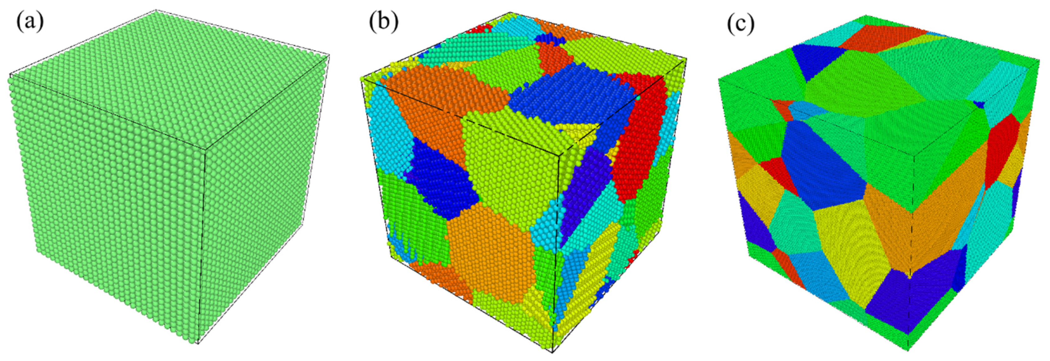
The Mie–Grüneisen EOS is usually applied to describe the behavior of metal materials under extreme shock compression, and the form of Mie–Grüneisen EOS can be expressed as follows [24]:

$$P-P_c=\frac{\gamma \left(V\right)}{V}\left(E-E_c\right)$$

(45)

$$P-P_H=\frac{\gamma \left(V\right)}{V}\left(E-E_H\right)$$

(46)

From the calculation results of P_H, E_H, P_c, E_c, and γ(V), the Mie–Grüneisen EOS could be obtained.

3. MD Simulation

The embedded-atom method (EAM) potential presented by Mendelev et al. [52] was used to conduct the MD simulation in this study. Three simulation models were established to investigate the dynamic characteristics of SC and NC iron under intensive shock conditions. The established models were based on bcc iron, and the shockwave direction is [001] in SC iron. Figure 1 shows the three simulation models. The NC models were built on the Voronoi algorithm in Atomsk [53]. The periodical boundary conditions were set in all directions for both SC and NC iron. To balance the calculation time and model size, the simulation system of SC iron was about 8.4 × 8.4 × 8.4 nm³ with 54,000 atoms. The model sizes of NC iron were about 10.9 × 10.9 × 10.9 nm³ with 111,195 atoms and 54.7 × 54.7 × 54.7 nm³ with 8,268,098 atoms. There were two grain sizes (GSs): 5 nm and 25 nm, which were chosen to study the GS effect in the shocking behavior.

First, the simulation system was equilibrated at 300 K for 10 ps in the NPT ensemble to ensure that the system reached a steady state in order to eliminate the residual stress. Then, the shockwave was examined using the MSST method under velocities of 6–11 km/s. Moreover, the computation time should be long enough to guarantee that the shockwave in the system reaches a steady state after the shock. Thus, the statistical results, such as the particle velocity, pressure, and temperature, could be obtained from the MD results.

4. Results and Discussion

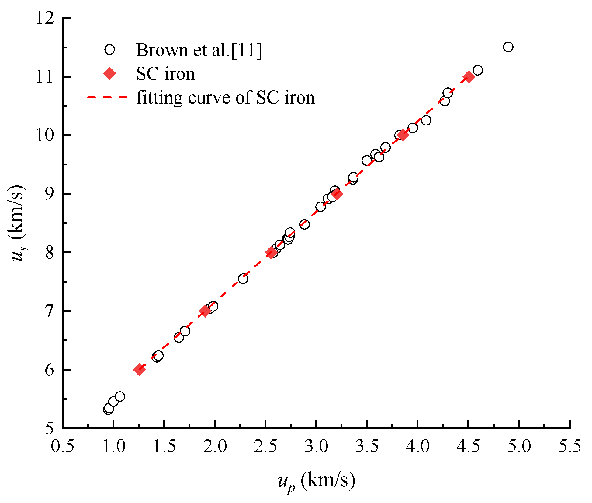
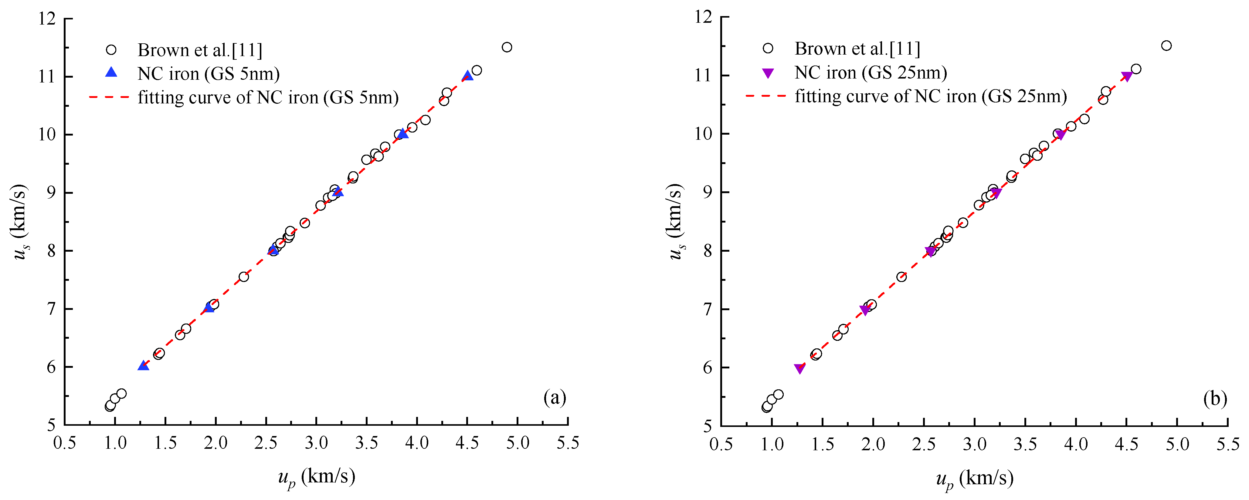
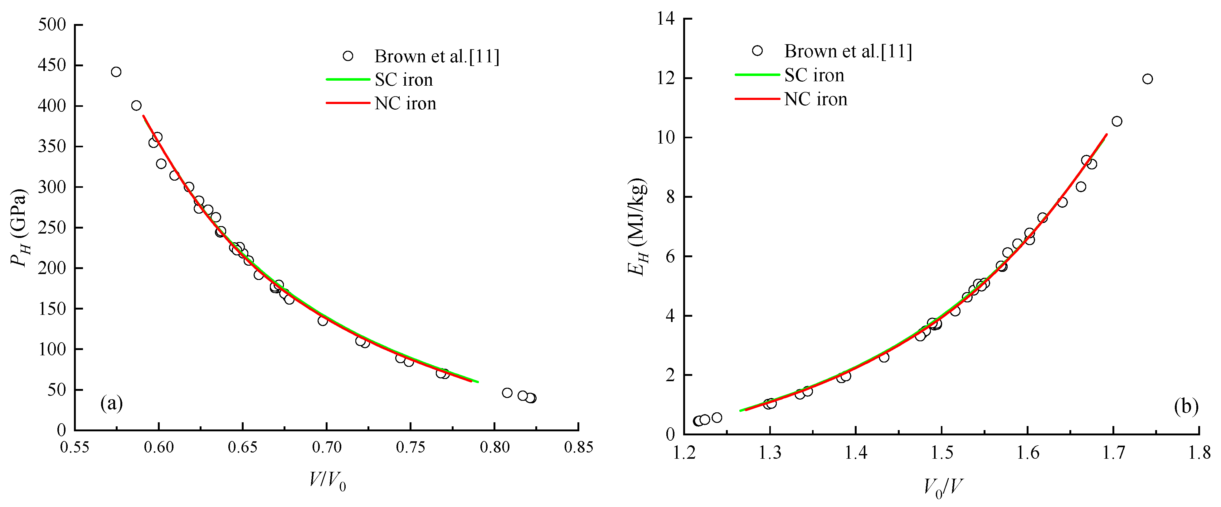
4.1. Shock Hugoniot Pressure and Internal Energy

According to the experimental Hugoniot data from Brown et al. [11], the shock velocity u_s ranged from 5.3 to 11.5 km/s at about 40–440 GPa. To ensure the stability of the MD simulation and evaluate the model validity, the velocity of u_s was set in the range of 6 to 11 km/s in this study. Figure 2 shows the relationship between u_s and u_p for SC iron obtained via the MSST method; there is a good agreement between the MD simulation results and experimental data. Moreover, the linear relationship between u_s and u_p is in excellent accordance with the data in Figure 2. The linear relationship is also consistent with the study by Prieto and Renero [54], which indicates that the relationship between u_s and u_p of iron below 5 megabars can be described by a linear relationship. For SC iron, the relationship between u_s and u_p is given as u_s = 4.071 + 1.538u_p. The relationship between u_s and u_p from the experimental data is expressed as u_s = 3.935 + 1.578u_p. The relative errors of C₀ and λ obtained from the MSST method and experiment were 3.3% and 2.6%, respectively, which proves the accuracy of the MD simulation.

To study the GS effect on the u_s–u_p relationship for NC iron, MD simulation was conducted at the same shock velocity as that of SC iron. The results are shown in Figure 3. The results of NC iron with different GS values are close. These discrete data are characterized by u_s = 4.011 + 1.552u_p and u_s = 4.01 + 1.553u_p for GS 5 nm and GS 25 nm, respectively. The relative error of C₀ and λ between GS 5 nm and GS 25 nm was less than 0.1%, and compared with the SC iron data, C₀ and λ were approximately equal to an error of <1.5%. The results indicate that the GS effect had little influence on the linear relationship between u_s and u_p for SC and NC iron, and it could be neglected in the case of NC iron.

The shock Hugoniot data obtained from MD simulations of SC and NC iron are listed in

Table 1. Hugoniot data for SC and NC iron determined by MD simulations at 300 K. An initial density of 7.85 g/cm³ is used.

Material	up (km/s)	us (km/s)	P (GPa)	ρ (g/cm3)
SC iron	1.25	6.00	60.84	9.92
	1.90	7.00	102.92	10.78
	2.55	8.00	158.50	11.53
	3.20	9.00	224.72	12.19
	3.85	10.00	301.71	12.77
	4.50	11.00	389.62	13.29
NC iron (GS 5 nm)	1.27	6.00	62.36	9.98
	1.92	7.00	105.82	10.82
	2.57	8.00	161.41	11.56
	3.21	9.00	227.10	12.21
	3.85	10.00	302.92	12.78
	4.50	11.00	388.85	13.29
NC iron (GS 25 nm)	1.28	6.00	62.34	9.98
	1.92	7.00	105.74	10.82
	2.56	8.00	161.22	11.56
	3.21	9.00	226.75	12.20
	3.85	10.00	302.34	12.77
	4.50	11.00	387.98	13.28

. As can be seen in Table 1, the particle velocity is high in NC iron below a shock velocity of 8.0 km/s, with a maximum difference of 2.5% between SC and NC iron. However, as the shock speed continues to grow, the difference in particle velocity becomes very small. At 11 km/s, the maximum shock pressure in SC and NC iron is 387.98–389.62 GPa. From [11], it can be found that the shock pressure is 361.8 GPa at a shock velocity of 10.7 km/s and 400.7 GPa at a shock velocity of 11.11 km/s. The MD results are within the range of the experimental data, which shows the accuracy of the simulation.

A detailed comparison of MD simulation results and experimental data is presented in

Table 2. C₀ and λ obtained from the linear relationship between u_s and u_p for SC and NC iron at 300 K. The initial density is 7.85 g/cm³ in both the experiment and MD simulation.

Material	Shock Velocity	C0 (km/s)	λ	Relative Error						Reference
				SC		NC (GS 5 nm)		NC (GS 25 nm)
				C0	λ	C0	λ	C0	λ
Commercial iron	5.3–11.5 km/s	3.935	1.578	3.34%	2.60%	1.89%	1.67%	1.87%	1.61%	[11]
SC	6–11 km/s	4.071	1.538	-	-	1.49%	0.90%	1.50%	0.96%	This work
NC (GS 5 nm)	6–11 km/s	4.011	1.552	1.49%	0.90%	-	-	0.02%	0.06%	This work
NC (GS 25 nm)	6–11 km/s	4.010	1.553	1.50%	0.96%	0.02%	0.06%	-	-	This work

. From Table 2, it can be observed that the volume sound speed C₀ in SC iron is higher than that in NC iron; however, the fitting parameter λ in SC iron is lower than that in NC iron, and the same characteristics are also observed in SC and NC Al [5]. The maximum relative error of C₀ between the experiment and SC iron is 3.34%, and the maximum relative error of NC iron is 1.89%. The difference of C₀ between SC and NC iron is ~1.5%, which is less than the difference with experiment data. The same characteristics in λ can be observed; the maximum relative error between the experiment and SC iron is 2.60%, and the maximum relative error of NC iron is 1.67%. The difference of λ between SC and NC iron is ~0.96%. The results indicate that a shock response difference between SC and NC iron does exist, but the difference is not very significant.

Based on the linear relationship obtained for SC and NC iron, the Hugoniot curve could be obtained using Equations (5) and (6). Figure 4 shows the Hugoniot curves of SC and NC iron. The black circle represents the results by Brown et al. [11], and the colored curves represent this work for SC and NC iron. Figure 4a shows that for V/V₀ > 0.6, the curves obtained through the MSST method agree well with the results of Brown et al. [11]; when V/V₀ < 0.6, the curves are approximately equal to the experiment results, and the deviation is less than 3%. Considering the insignificant error of C₀ and λ for SC and NC iron, there is no noticeable difference between the three curves in Figure 4a. As shown in Figure 4b, the internal energies obtained in the MD simulation and experiment were almost the same; when V₀/V = 1.7, the internal energy of SC iron was smaller than that of NC iron, and the deviation at V₀/V = 1.7 was 0.5%. The results not only prove the reliability of the linear relationship between u_s and u_p but also show the EAM potential for iron in the MD simulation. In addition, the results signify that the MD results are appropriate for describing the cold pressure, the cold energy, the melting temperature, and the Mie–Grüneisen EOS.

4.2. Cold Pressure and Cold Energy

Based on the C₀ and λ obtained from the Hugoniot data, the material constants for calculating cold pressure and cold energy in Equations (18)–(21) could be obtained. The values are presented in

Table 3. Material constants for calculating cold pressure and cold energy.

Material Constants	V0 (g/cm3)	${\mathit{C}}_0^{\prime }(\mathbf{km}/\mathbf{s})$	λ′	Q (GPa)	q	A (GPa)	B
Experiment	0.127	4.010	1.581	41.245	11.192	87.662	4.325
SC iron	0.127	4.094	1.540	46.473	10.716	97.319	4.162
NC iron	0.127	4.093	1.541	44.238	10.894	93.170	4.223

.

Figure 5 and Figure 6 compare the cold pressure P_c and cold energy E_c between SC and NC iron, with the experimental data as a reference. The solid and dashed curves represent P_c and E_c obtained using the Born–Mayer and Morse potentials, respectively. The results from the Born–Mayer and Morse potentials presented the same increasing trend: P_c and E_c increased with volume compression (V_0K/V), which presented a sharp increment at higher compression.

At V_0K/V less than 1.3, the curves of P_c agree well with each other. The result shows that the cold energies described by the Born–Mayer and Morse potentials are basically the same in the low-compression region. When the V_0K/V is above 1.3, the P_c curves gradually deviate from each other, and the P_c curves obtained by the Born–Mayer potential gradually become larger. The relative error of P_c was about 10% when V_0K/V was 2.0. Irrespective of the potential function used, the cold pressure curve of SC iron was above that of the NC iron. This indicates that the cold pressure of SC iron was higher than that of NC iron, although the difference was quite small.

Under V_0K/V of less than 1.4, the cold energy curves agree well with each other, as the cold pressures obtained by the Born–Mayer and Morse potentials in the low-compression region are approximately equal. Under V_0K/V of above 1.4, the E_c curves gradually deviate from each other. The cold energy obtained by the Born–Mayer potential is larger than that from the Morse potential, and the same trend was found for the cold pressure. The relative error of E_c is about 7% when V_0K/V is 2.0. Furthermore, the cold energy in the SC iron is larger than that of the NC iron in both Born–Mayer and Morse potentials.

4.3. Grüneisen Coefficient

The material constant λ in SC and NC iron was used to calculate the γ₀ of the Slater, Dugdale–Macdonald, and free-volume models through Equations (30)–(32). Subsequently, γ₀(V) was substituted into Equations (34)–(38) to obtain γ(V), and the experimental data were used for comparison. Figure 7 shows the results of γ(V) from different empirical and theoretical models.

Equations (34)–(38) are commonly used empirical models for calculating γ(V) at high pressure. From Figure 7, it can be seen that the Grüneisen coefficient γ(V) first rapidly decreased and then slowly dropped as the V₀/V increased. At high compression, the difference between SC and NC results became smaller; this indicates that the microstructure has little effect on γ(V) under high pressure. Equation (38) is suitable for low-compression data, that is, V₀/V up to 1.5, and is free with λ; thus, different models do not affect their results. With Equation (38) as a reference, when V₀/V = 1.0, the initial value of γ₀ is γ_f (V₀) < γ_DM(V₀) < γ_S(V₀). For all three models, the γ(V) obtained by the experimental data (solid curve) is at the top followed by that for the NC iron (dash curve), and that for the SC iron (dot curve) is at the bottom due to the difference between the λ values. Compared with the results from Equations (35)–(38), the results from Equation (34) (black curves) show a more significant downward trend with the increase in V₀/V. This shows that the γ(V) calculated using Equation (34) has the maximum change rate with the increase in V₀/V. The results from Equation (35)–(38) present a similar trend in predicting γ(V).

Equation (38) (magenta curve) is free of λ, and it has been proven to agree well with the experimental data under V₀/V up to 1.5 [49]. The γ(V) obtained using the free-volume model has the smallest difference under V₀/V up to 1.5. When V₀/V is 1.5, the γ(V) obtained by Equation (37) (cyan curve) intersects with the magenta curve. This indicates that Equation (27) is applicable to characterize the γ(V) of iron at higher compression compared with other expressions. This has also been proved by Jacobs and Schmid-Fetzer [48]. In Figure 7c, the green curve is closer to the cyan curve than other curves. The result shows that Equation (36) (green curve) is more suitable than other expressions for describing γ(V). The relative error of the green curve is 7.8% at V₀/V = 2.0.

4.4. Melting Temperature

Based on the Grüneisen coefficient and the Lindemann law, the melting temperature T_m can be obtained. In this study, γ₀ is calculated via the free-volume model with Equation (26), and T_m is predicted by Equations (40)–(44). The relationship between T_m and pressure is illustrated in Figure 8, together with experimental data [35,55,56,57,58,59,60,61,62,63] and theoretical data [64,65,66,67,68].

As shown in Figure 8, the temperature rises quickly to the melting point because of the adiabatic process under shock compression, and T_m shows an increasing trend as the pressure increases. The results from Equations (41), (42) and (44) present a similar and close trend; the red curve at the top corresponds to Equation (41), while the green curve at the bottom corresponds to Equation (43), and the maximum error is 29.5% at 450 GPa. Moreover, the melting temperature in SC iron is a little lower than that in NC iron; the maximum error is 2.5% at 450 GPa.

At lower pressure (<100 GPa), all curves except the green one are very close; this shows that the prediction abilities of Equations (40)–(42) and (44) in the low-compression area are almost the same. It can be found that T_m calculated by Equations (40) and (44) agrees well with DAC experimental data in [57], and T_m calculated by Equation (43) agrees well with DAC experimental data in [59,60,62]. T_m calculated by Equations (41) and (42) is little higher than that obtained from DFT calculations [64,65,66]. However, the difference between the results gradually increased at higher pressure (>100 GPa). The increasing trend indicates that in the low-compression area, the effect of γ₀ on T_m is insignificant; the effect of γ₀ on T_m becomes more significant with increasing pressure. This feature shows the opposite trend compared with the γ(V) results. In Figure 8, it can be found that the DAC experimental data of Anzellini et al. [35], the theoretical data obtained by MD calculations conducted by Zhang et al. [58], and DFT calculations conducted by Alfè et al. [64,65,66] are in good agreement. Thus, the orange melting curve obtained by the DAC experiment up to ~350 GPa was chosen as the main reference in this study. The results obtained from Equations (40)–(44) are similar to the orange line, although there are some differences in the results. At lower pressure (<100 GPa), the black line obtained by Equation (40) is the closest to the orange line, and the green line (Equation (43)) and purple line (Equation (44)) slightly deviate from the orange line. This indicates that Equation (40) can be used to approximately predict T_m under 100 GPa. In the entire pressure range, the orange line is within the calculation result from Equation (44) at pressure less than 300 GPa; the result obtained from Equation (44) is lower than the orange line above 300 GPa. This result shows that the calculation results under 300 GPa can cover the experimental data, and the results obtained at higher pressures are lower than the experimental data.

4.5. Mie–Grüneisen Equation of State

The Mie–Grüneisen EOS can be obtained from Equations (45) and (46) with the Hugoniot curve (Equation (45)) and the cold curve (Equation (46)) as the reference curves. The Hugoniot curve is obtained via MD simulation. Based on previous analysis, the Grüneisen coefficient γ in this study is calculated by Equations (32) and (36). The cold pressure and cold energy are calculated from the Born–Mayer potential. Figure 9 shows the Mie–Grüneisen EOS of iron in 3D contour form of SC iron based on the cold pressure and cold energy, with the Hugoniot relations as the reference.

The Mie–Grüneisen EOS is described in the pressure–specific volume–internal energy (P-V-E) space. In the front view, the whole Mie–Grüneisen EOS space presents a concave surface characteristic, as shown in Figure 9. The maximum pressure of EOS calculated from the cold curve or the Hugoniot curve as the reference will be different. The maximum pressure when the Hugoniot relations are utilized as the reference is ~200 GPa higher than that when the cold pressure and cold energy are the references. The results indicate that the reference data have a certain impact on the surface characteristic and values of the Mie–Grüneisen EOS.

5. Conclusions

In this study, a micromechanical approach for determining the Mie–Grüneisen EOS parameters of iron under the Hugoniot states was investigated using the MSST method in MD simulation, and the shock Hugoniot, cold curve, melting temperature, and Grüneisen coefficient are also discussed. The simulation results show that the difference between the linear relationships of the shock Huguenot of SC and NC iron was insignificant, and both agree well with the experiment data. Compared with the results at GS 5 nm and 25 nm, the GS effect of iron was not significant at high pressures. The difference between the Born–Mayer potential and the Morse potential in calculating the cold pressure was almost the same as that in calculating the cold energy, but the cold pressure and cold energy in SC iron were a little higher than those in NC iron. As the pressure increased, the Grüneisen coefficient gradually decreased, while the melting temperature gradually increased; the two trends were opposite. The Grüneisen coefficient γ is calculated by Equations (16c) and (18c), which have a better performance in this study. The Mie–Grüneisen EOS presented a concave surface characteristic in 3D contour space; the pressure with the Hugoniot curve as the reference was higher than that with the cold curve as the reference, which indicates that different reference curves have a certain impact on the surface characteristic and values of Mie–Grüneisen EOS. The research results in this paper prove the feasibility of the MSST method and provide a reference for studying the EOS of other metals under high pressures. Materials in practical applications are very complex and contain various impurities and defects, and both impurities and defects affect their properties. We examined pure SC iron and perfect NC iron in this study with the MSST method. In future work, we will consider impurities and defects to study the dynamic response characteristics of materials under more complex conditions.

References

1. Batani, D.; Morelli, A.; Tomasini, M.; Benuzzi-Mounaix, A.; Philippe, F.; Koenig, M.; Marchet, B.; Masclet, I.; Rabec, M.; Reverdin, C.; et al. Equation of state data for iron at pressures beyond 10 Mbar. Phys. Rev. Lett. 2002, 88, 235502. [Google Scholar] [CrossRef]
2. Hai-Jun, H.; Fu-Qian, J.; Ling-Cang, C.; Yan, B. Grüneisen Parameter along Hugoniot and Melting Temperature of ε-Iron: A Result from Thermodynamic Calculations. Chin. Phys. Lett. 2005, 22, 836. [Google Scholar] [CrossRef]
3. Dorogokupets, P.I.; Dymshits, A.M.; Litasov, K.D.; Sokolova, T.S. Thermodynamics and Equations of State of Iron to 350 GPa and 6000 K. Sci. Rep. 2017, 7, 41863. [Google Scholar] [CrossRef] [Green Version]
4. Joshi, R.H.; Bhatt, N.K.; Thakore, B.Y.; Vyas, P.R.; Jani, A.R. Grüneisen parameter and equations of states for copper–High pressure study. Comput. Condens. Matter 2018, 15, 79–84. [Google Scholar] [CrossRef]
5. Yang, X.; Zeng, X.; Pu, C.; Chen, W.; Chen, H.; Wang, F. Molecular dynamics modeling of the Hugoniot states of aluminum. AIP Adv. 2018, 8, 105212. [Google Scholar] [CrossRef] [Green Version]
6. Shao, J.L.; He, A.M.; Wang, P. Atomistic simulations on the dynamic properties of shock and release melting in single crystal Al. Comput. Mater. Sci. 2018, 151, 240–245. [Google Scholar] [CrossRef]
7. Nagayama, K. Extended Rice-Walsh equation of state for metals based on shock Hugoniot data for porous samples. J. Appl. Phys. 2017, 121, 175902. [Google Scholar] [CrossRef]
8. Barker, L.M. Alpha-phase Hugoniot of iron. J. Appl. Phys. 1975, 46, 2544–2547. [Google Scholar] [CrossRef]
9. Thomas, S.A.; Hawkins, M.C.; Matthes, M.K.; Gray, G.T., III; Hixson, R.S. Dynamic strength properties and alpha-phase shock Hugoniot of iron and steel. J. Appl. Phys. 2018, 123, 175902. [Google Scholar] [CrossRef] [Green Version]
10. Kadau, K.; Germann, T.C.; Lomdahl, P.S.; Holian, B.L. Microscopic view of structural phase transitions induced by shock waves. Science 2002, 296, 1681–1684. [Google Scholar] [CrossRef] [PubMed] [Green Version]
11. Brown, J.M.; Fritz, J.N.; Hixson, R.S. Hugoniot data for iron. J. Appl. Phys. 2000, 88, 5496–5498. [Google Scholar] [CrossRef]
12. Zaretsky, E.B. Shock response of iron between 143 and 1275 K. J. Appl. Phys. 2009, 106, 023510. [Google Scholar] [CrossRef]
13. Liu, X.; Mashimo, T.; Kawai, N.; Sano, T.; Zhou, X. Isotropic phase transition of single-crystal iron (Fe) under shock compression. J. Appl. Phys. 2018, 124, 215101. [Google Scholar] [CrossRef]
14. Sjostrom, T.; Crockett, S. Quantum molecular dynamics of warm dense iron and a five-phase equation of state. Phys. Rev. E 2018, 97, 053209. [Google Scholar] [CrossRef] [Green Version]
15. Kadau, K.; Germann, T.C.; Lomdahl, P.S.; Holian, B.L. Atomistic simulations of shock-induced transformations and their orientation dependence in bcc Fe single crystals. Phys. Rev. B 2005, 72, 064120. [Google Scholar] [CrossRef]
16. Kadau, K.; Germann, T.C.; Lomdahl, P.S.; Albers, R.C.; Wark, J.S.; Higginbotham, A.; Holian, B.L. Shock waves in polycrystalline iron. Phys. Rev. Lett. 2007, 98, 135701. [Google Scholar] [CrossRef] [Green Version]
17. Belkheeva, R.K. Equation of state for a highly porous material. High Temp. 2015, 53, 348–357. [Google Scholar] [CrossRef]
18. Khishchenko, K.V. Equation of state of sodium for modeling of shock-wave processes at high pressures. Math. Montisnigri 2017, 40, 140–147. [Google Scholar]
19. Maevskii, K.K.; Kinelovskii, S.A. Numerical simulation of thermodynamic parameters of high-porosity copper. Tech. Phys. 2019, 64, 1090–1095. [Google Scholar] [CrossRef]
20. Hallajisany, M.; Zamani, J.; Albelda Vitoria, J. Numerical and theoretical determination of various materials Hugoniot relations based on the equation of state in high-temperature shock loading. High Press. Res. 2019, 39, 666–690. [Google Scholar] [CrossRef]
21. Maevskii, K.K.; Kinelovskii, S.A. Modeling of High-Porosity Copper-Based Mixtures under Shock Loading. J. Appl. Mech. Tech. Phys. 2019, 60, 612–619. [Google Scholar] [CrossRef]
22. Khishchenko, K.V. Equation of state for niobium at high pressures. Math. Montisnigri 2020, 47, 119–123. [Google Scholar] [CrossRef]
23. Gilev, S.D. Low-parametric equation of state of aluminum. High Temp. 2020, 58, 166–172. [Google Scholar] [CrossRef]
24. Heuzé, O. General form of the Mie–Grüneisen equation of state. C. R. Mec. 2012, 340, 679–687. [Google Scholar] [CrossRef]
25. Zhang, X.F.; Qiao, L.; Shi, A.S.; Zhang, J.; Guan, Z.W. A cold energy mixture theory for the equation of state in solid and porous metal mixtures. J. Appl. Phys. 2011, 110, 013506. [Google Scholar] [CrossRef]
26. Patel, N.N.; Sunder, M. High pressure melting curve of osmium up to 35 GPa. J. Appl. Phys. 2019, 125, 055902. [Google Scholar] [CrossRef]
27. Slater, J.C. Introduction to Chemical Physics; Chapter XIII; McGraw-Hill: New York, NY, USA, 1939. [Google Scholar]
28. Dugdale, J.S.; MacDonald, D.K.C. The thermal expansion of solids. Phys. Rev. 1953, 89, 832. [Google Scholar] [CrossRef]
29. Vashchenko, V.Y.; Zubarev, V.N. Concerning the Grüneisen constant. Fiz. Tverd. Tela 1963, 5, 886–890. [Google Scholar]
30. Al’tshuler, L.V. Use of shock waves in high-pressure physics. Phys. Uspekhi 1965, 8, 52–91. [Google Scholar] [CrossRef]
31. Cui, G.; Yu, R. Volume and pressure dependence of Grüneisen parameter γ for solids at high temperatures. Phys. B Condens. Matter 2007, 390, 220–224. [Google Scholar] [CrossRef]
32. Sha, X.; Cohen, R.E. Lattice dynamics and thermodynamics of bcc iron under pressure: First-principles linear response study. Phys. Rev. B 2006, 73, 104303. [Google Scholar] [CrossRef] [Green Version]
33. Xi-Jun, L.; Xian-Ming, Z.; Fan-Hou, W.; Fu-Qian, J. Restudy of Grüneisen Parameter of Iron in the Pressure Range of 90–160 GPa. Chin. Phys. Lett. 2001, 18, 85. [Google Scholar] [CrossRef]
34. Errandonea, D. High-pressure melting curves of the transition metals Cu, Ni, Pd, and Pt. Phys. Rev. B 2013, 87, 054108. [Google Scholar] [CrossRef]
35. Anzellini, S.; Dewaele, A.; Mezouar, M.; Loubeyre, P.; Morard, G. Melting of iron at Earth’s inner core boundary based on fast X-ray diffraction. Science 2013, 340, 464–466. [Google Scholar] [CrossRef]
36. Bouchet, J.; Mazevet, S.; Morard, G.; Guyot, F.; Musella, R. Ab initio equation of state of iron up to 1500 GPa. Phys. Rev. B 2013, 87, 094102. [Google Scholar] [CrossRef]
37. Barton, M.A.; Stacey, F.D. The Grüneisen parameter at high pressure: A molecular dynamical study. Phys. Earth Planet. Inter. 1985, 39, 167–177. [Google Scholar] [CrossRef]
38. Maillet, J.B.; Mareschal, M.; Soulard, L.; Ravelo, R.; Lomdahl, P.S.; Germann, T.C.; Holian, B.L. Uniaxial Hugoniostat: A method for atomistic simulations of shocked materials. Phys. Rev. E 2000, 63, 016121. [Google Scholar] [CrossRef]
39. Vočadlo, L.; Dobson, D.P.; Wood, I.G. An ab initio study of nickel substitution into iron. Earth Planet. Sci. Lett. 2006, 248, 147–152. [Google Scholar] [CrossRef]
40. Reed, E.J.; Fried, L.E.; Joannopoulos, J.D. A method for tractable dynamical studies of single and double shock compression. Phys. Rev. Lett. 2003, 90, 235503. [Google Scholar] [CrossRef] [Green Version]
41. Wen, P.; Demaske, B.; Spearot, D.E.; Phillpot, S.R.; Tao, G. Effect of the initial temperature on the shock response of Cu50Zr50 bulk metallic glass by molecular dynamics simulation. J. Appl. Phys. 2021, 129, 165103. [Google Scholar] [CrossRef]
42. Dewapriya, M.A.N.; Miller, R.E. Energy absorption mechanisms of nanoscopic multilayer structures under ballistic impact loading. Comput. Mater. Sci. 2021, 195, 110504. [Google Scholar] [CrossRef]
43. Chen, J.; Chen, W.; Chen, S.; Zhou, G.; Zhang, T. Shock Hugoniot and Mie-Grüneisen EOS of TiAl alloy: A molecular dynamics approach. Comput. Mater. Sci. 2020, 174, 109495. [Google Scholar] [CrossRef]
44. Born, M.; Mayer, J.E. Zur Gittertheorie der Ionenkristalle. Z. Phys. 1932, 75, 1–18. [Google Scholar] [CrossRef]
45. Morse, P.M. Diatomic molecules according to the wave mechanics. II. Vibrational levels. Phys. Rev. 1929, 34, 57. [Google Scholar] [CrossRef]
46. Eliezer, S.; Ghatak, A.; Hora, H. Fundamentals of Equations of State; World Scientific: Singapore, 2002; pp. 197–207. [Google Scholar]
47. Segletes, S.B.; Walters, W.P. On theories of the Grüneisen parameter. J. Phys. Chem. Solids 1998, 59, 425–433. [Google Scholar] [CrossRef]
48. Jacobs, M.H.G.; Schmid-Fetzer, R. Thermodynamic properties and equation of state of fcc aluminum and bcc iron, derived from a lattice vibrational method. Phys. Chem. Miner. 2010, 37, 721–739. [Google Scholar] [CrossRef]
49. Burakovsky, L.; Preston, D.L. An analytic model of the Grüneisen parameter all densities. J. Phys. Chem. Solids 2004, 65, 1581–1587. [Google Scholar] [CrossRef] [Green Version]
50. Ross, M. Generalized Lindemann melting law. Phys. Rev. 1969, 184, 233. [Google Scholar] [CrossRef]
51. Haynes, W.M. CRC Handbook of Chemistry and Physics; CRC Press: Boca Raton, FL, USA, 2014. [Google Scholar]
52. Mendelev, M.I.; Han, S.; Srolovitz, D.J.; Ackland, G.J.; Sun, D.Y.; Asta, M. Development of new interatomic potentials appropriate for crystalline and liquid iron. Philos. Mag. 2003, 83, 3977–3994. [Google Scholar] [CrossRef]
53. Hirel, P. Atomsk: A tool for manipulating and converting atomic data files. Comput. Phys. Commun. 2015, 197, 212–219. [Google Scholar] [CrossRef]
54. Prieto, F.E.; Renero, C. Equation for the Shock Adiabat. J. Appl. Phys. 1970, 41, 3876–3883. [Google Scholar] [CrossRef]
55. Boehler, R. Temperatures in the Earth’s core from melting-point measurements of iron at high static pressures. Nature 1993, 363, 534–536. [Google Scholar] [CrossRef]
56. Nguyen, J.H.; Holmes, N.C. Melting of iron at the physical conditions of the Earth’s core. Nature 2004, 427, 339–342. [Google Scholar] [CrossRef] [PubMed]
57. Williams, Q.; Jeanloz, R.; Bass, J.; Svendsen, B.; Ahrens, T.J. The melting curve of iron to 250 gigapascals: A constraint on the temperature at Earth’s center. Science 1987, 236, 181–182. [Google Scholar] [CrossRef]
58. Zhang, W.J.; Liu, Z.Y.; Liu, Z.L.; Cai, L.C. Melting curves and entropy of melting of iron under Earth’s core condi-tions. Phys. Earth Planet. Inter. 2015, 244, 69–77. [Google Scholar] [CrossRef]
59. Jackson, J.M.; Sturhahn, W.; Lerche, M.; Zhao, J.; Toellner, T.S.; Alp, E.E.; Sinogeikin, S.V.; Bass, J.D.; Murphy, C.A.; Wicks, J.K. Melting of compressed iron by monitoring atomic dynamics. Earth Planet. Sci. Lett. 2013, 362, 143–150. [Google Scholar] [CrossRef]
60. Shen, G.; Prakapenka, V.B.; Rivers, M.L.; Sutton, S.R. Structure of liquid iron at pressures up to 58 GPa. Phys. Rev. Lett. 2004, 92, 185701. [Google Scholar] [CrossRef]
61. Swartzendruber, L.J. The Fe (Iron) system. Bull. Alloy Phase Diagr. 1982, 3, 161–165. [Google Scholar] [CrossRef]
62. Ma, Y.; Somayazulu, M.; Shen, G.; Mao, H.K.; Shu, J.; Hemley, R.J. In situ X-ray diffraction studies of iron to Earth-core conditions. Phys. Earth Planet. Inter. 2004, 143–144, 455–467. [Google Scholar] [CrossRef]
63. Brown, J.M.; McQueen, R.G. Phase transitions, Grüneisen parameter, and elasticity for shocked iron between 77 GPa and 400 GPa. J. Geophys. Res. 1986, 91, 7485–7494. [Google Scholar] [CrossRef]
64. Alfè, D. Temperature of the inner-core boundary of the Earth: Melting of iron at high pressure from first-principles coexistence simulations. Phys. Rev. B 2009, 79, 060101. [Google Scholar] [CrossRef] [Green Version]
65. Alfè, D.; Cazorla, C.; Gillan, M.J. The kinetics of homogeneous melting beyond the limit of superheating. J. Chem. Phys. 2011, 135, 024102. [Google Scholar] [CrossRef] [PubMed] [Green Version]
66. Alfè, D.; Price, G.; Gillan, M. Iron under Earth’s core conditions: Liquid-state thermodynamics and high-pressure melting curve from ab initio calculations. Phys. Rev. B 2002, 65, 165118. [Google Scholar] [CrossRef] [Green Version]
67. Belonoshko, A.B.; Ahuja, R.; Johansson, B. Quasi–ab initio molecular dynamic study of Fe melting. Phys. Rev. Lett. 2000, 84, 3638–3641. [Google Scholar] [CrossRef]
68. Luo, F.; Cheng, Y.; Chen, X.R.; Cai, L.C.; Jing, F.Q. The melting curves and entropy of iron under high pressure. J. Chem. Eng. Data 2011, 56, 2063–2070. [Google Scholar] [CrossRef]
Figure 1. Configurations of (a) SC iron and (b) NC iron with GS of 5 nm and (c) NC iron with GS of 25 nm. Separate grains are distinguished by different colors.
Crystals 11 00664 g001
Figure 2. The relation between us and up for SC at 300 K (the linear fitting curve is applied to the MD results; experimental data are shown for comparison).
Crystals 11 00664 g002
Figure 3. The relationship between us and up for NC iron at 300 K: (a) NC iron with GS 5 nm (b) NC iron with GS 25 nm (the linear fitting curve is applied to the MD results; experimental data are shown for comparison).
Crystals 11 00664 g003
Figure 4. The Hugoniot curves of SC and NC iron: (a) PH curve; (b) EH curve.
Crystals 11 00664 g004
Figure 5. The cold pressures of SC and NC iron.
Crystals 11 00664 g005
Figure 6. The cold energy of SC and NC iron.
Crystals 11 00664 g006
Figure 7. The relationship between the Grüneisen coefficient γ(V) and V0/V. (a) γ(V) calculated from the Slate model, (b) γ(V) calculated from the Dugdale-MacDonald model, (c) γ(V) calculated from the Free-volume model.
Crystals 11 00664 g007
Figure 8. Comparison of the melting temperature of iron from present calculations with previous studies [35,55,56,57,58,59,60,61,62,63,64,65,66,67,68].
Crystals 11 00664 g008
Figure 9. Mie–Grüneisen EOS in P-V-E form with reference from the cold curve (a) and the Hugoniot curve (b).
Crystals 11 00664 g009