Mathematical Model for Metal Transfer Study in Additive Manufacturing with Electron Beam Oscillation

Abstract

A computer model has been developed to investigate the processes of heat and mass transfer under the influence of concentrated energy sources on materials with specified thermophysical characteristics, including temperature-dependent ones. The model is based on the application of the volume of fluid (VOF) method and finite-difference approximation of the Navier–Stokes differential equations formulated for a viscous incompressible medium. The “predictor-corrector” method has been used for the coordinated determination of the pressure field which corresponds to the continuity condition and the velocity field. The modeling technique of the free liquid surface and boundary conditions has been described. The method of calculating surface tension forces and vapor recoil pressure has been presented. The algorithm structure is given, the individual modules of which are currently implemented in the Microsoft Visual Studio environment. The model can be applied for studying the metal transfer during the deposition processes, including the processes with electron beam spatial oscillation. The model was validated by comparing the results of computational experiments and images obtained by a high-speed camera.

1. Introduction

The process of metal transfer under the influence of concentrated heating sources is one of the most difficult objects to study. This is due to high temperature gradients and high metal flow rates in the molten pool region, as well as the presence of high-intensity optical radiation and metal vapors, which complicate video shooting or the use of thermal imaging technology [1,2]. In addition, experimental research methods do not allow obtaining information on the distribution of flow velocities, temperature, and pressure in the volume of a molten pool. However, they provide indirect data about the processes occurring on the surface. Main interest in the study of general patterns of metal transfer has increased recently. It can be associated with the advent of technologies for additive manufacturing of products made of metal materials supplied both in powder form [3,4,5,6] and in wire form [7,8].

In this regard, mathematical modeling methods are rather relevant due to the fact that they can be used to obtain the data on processes that have occurred in a molten pool by conducting computational experiments. Today, a large number of papers have been published on the analysis of heat and mass transfer phenomena in the implementation of additive technologies [9,10,11].

National Research University “Moscow Power Engineering Institute” is faced with the task of creating a universal software package for wire-based electron-beam additive manufacturing systems, which could be used not only for modeling heat and mass transfer but would also be suitable for integration into a process control system. In addition, the mathematical model intended for the analysis of hydrodynamic processes included in this complex should provide the study of the motion of the free surface of the melt under the influence of an oscillating beam. For example, when using the saw-tooth shape of the deflecting coils current and a sufficient degree of beam focusing, it is possible to ensure directional metal transfer; which, in turn, allows the formation of deposited layers of greater height and smaller width from the filler material than in the absence of oscillation [12]. To study the transfer process, it is necessary to develop a model that takes into account the effect of surface tension forces and vapor recoil pressure on the free metal surface.

However, for a structured description of the model proposed in this paper, it is necessary to refer to the basic principles of transfer phenomena numerical modeling. In the 1970s and 1980s, the theoretical foundations for the numerical solution of multidimensional problems of hydrodynamics were laid [13,14] and the first samples of applied software were created—SIMPLE, SIMPLER, and others [13,15,16]. At the same time, the basic methods of interpolation of media interface free surface boundary were proposed [17,18]. The development of computer technology in the following decades led to a sharp increase in interest according to the problems of computational fluid dynamics and heat transfer, which caused both the creation of commercial packages and the emergence of many specialized programs [19,20]. Generally, they presented in the form of open-source software for universal programming environments such as Visual C, C++, C#, Delphi, VB.NET, etc.

The use of the described world experience and the results of our own research has made it possible to create software for studying and predicting the additive manufacturing process. The modular software design ensures its adaptation for solving various problems, for example, the study of the process of electron scattering [21] or the synthesis of control algorithms [22]. In this paper, it is proposed to adapt the algorithms created at NRU “MPEI” to study the process of directed metal transfer under the effect of the vapor recoil pressure arising from the action of an oscillating beam on the melt.

2. Description of the Model and Methods Used

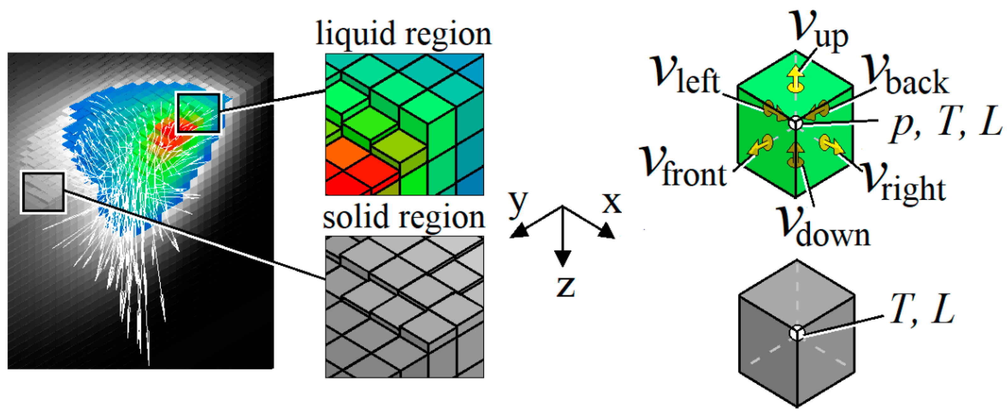
The model is implemented for a fixed or Eulerian coordinate system (Figure 1). A cubic grid with a “staggered” structure is used [13]. When using such a grid in the centers of cubic control volumes, scalar values are calculated—pressure p, Pa; temperature T, K; dimensionless function of the control volume relative filling L. Projections of metal flow velocities on Cartesian axes are calculated on the faces of the cubic control volume; they are conventionally shown in Figure 1 as v_left, v_right, v_back, v_front, v_up, and v_down.

To describe the process of metal transfer in a molten pool, the Navier–Stokes equations describing the flow of a viscous incompressible liquid are used. The equation of motion relates the acceleration imparted to the medium at the considered fixed point with internal and external forces acting on the fluid

$$\frac{\partial \overrightarrow{v}}{\partial t}+\left(\overrightarrow{v}\cdot \nabla \right)\overrightarrow{v}=-\frac{1}{\rho }\nabla p+\mu \nabla \left(\nabla \overrightarrow{v}\right)+\frac{{\overrightarrow{f}}_{st}}{\rho }+\frac{{\overrightarrow{f}}_{rec}}{\rho }+\overrightarrow{g} ,$$

(1)

where $\overrightarrow{v}$ is liquid metal flow velocity vector, m/s; t is time, s; ρ is metal density, kg/m³; µ is kinematic viscosity, m²/s; ${\overrightarrow{f}}_{st}$ and ${\overrightarrow{f}}_{rec}$ are volumetric equivalents of surface tension forces and vapor recoil pressure, respectively, N/m³; $\overrightarrow{g}$ is gravitational acceleration, m/s².

To create an algorithm using an explicit difference scheme, it is necessary to write Equation (1) in the form of projections on Cartesian axes:

$$\begin{gathered} \frac{\partial v_x}{\partial t}+v_x\frac{\partial v_x}{\partial x}+v_y\frac{\partial v_x}{\partial y}+v_z\frac{\partial v_x}{\partial z}=-\frac{1}{\rho }\frac{\partial p}{\partial x}+\mu \left(\frac{{\partial }^2{v}_x}{\partial x^2}+\frac{{\partial }^2{v}_x}{\partial y^2}+\frac{{\partial }^2{v}_x}{\partial z^2}\right)+\frac{f_{\mathit{st}.x}}{\rho }+\frac{f_{rec.x}}{\rho } \\ \frac{\partial v_y}{\partial t}+v_x\frac{\partial v_y}{\partial x}+v_y\frac{\partial v_y}{\partial y}+v_z\frac{\partial v_y}{\partial z}=-\frac{1}{\rho }\frac{\partial p}{\partial y}+\mu \left(\frac{{\partial }^2{v}_y}{\partial x^2}+\frac{{\partial }^2{v}_y}{\partial y^2}+\frac{{\partial }^2{v}_y}{\partial z^2}\right)+\frac{f_{\mathit{st}.x}}{\rho }+\frac{f_{rec.y}}{\rho }, \\ \frac{\partial v_z}{\partial t}+v_x\frac{\partial v_z}{\partial x}+v_y\frac{\partial v_z}{\partial y}+v_z\frac{\partial v_z}{\partial z}=-\frac{1}{\rho }\frac{\partial p}{\partial z}+\mu \left(\frac{{\partial }^2{v}_z}{\partial x^2}+\frac{{\partial }^2{v}_z}{\partial y^2}+\frac{{\partial }^2{v}_z}{\partial z^2}\right)+\frac{f_{\mathit{st}.z}}{\rho }+\frac{f_{rec.z}}{\rho }+g \end{gathered}$$

(2)

where v_x, v_y, v_z, f_st.x, f_st.y, f_st.z, f_rec.x, f_rec.y, and f_rec.z are projections of velocity vectors $\overrightarrow{v}$ and volumetric forces ${\overrightarrow{f}}_{st}$ and ${\overrightarrow{f}}_{rec}$ on the corresponding coordinate axes. The gravitational acceleration in the last equation coincides in the direction with the z axis.

To calculate the pressure field satisfying the continuity equation for the case of an incompressible fluid, it is necessary to use one of the splitting schemes by physical factors [13,23]. Such methods can be conditionally combined under the name ‘predictor–corrector’ since the full approximation of the velocity field is provided only at the correction stage after the pressure field iterative calculation. The most well-known method for solving such a problem, which can be described by Equations (3)–(7), is the SIMPLE algorithm (Semi-Implicit Method for Pressure Linked Equations [13]). At the first stage, if the pressure field is unknown, the speed increment is calculated due to the action of all factors except pressure. This stage is described by the equation

$$\frac{{\overrightarrow{v}}^p-{\overrightarrow{v}}^{*}}{\Delta t}=-\left({\overrightarrow{v}}^{*}·\nabla \right){\overrightarrow{v}}^{*}+\mu \nabla \left(\nabla {\overrightarrow{v}}^{*}\right)+\frac{{\overrightarrow{f}}_{st}}{\rho }+\frac{{\overrightarrow{f}}_{rec}}{\rho }+\overrightarrow{g} ,$$

(3)

where ${\overrightarrow{v}}^{*}$ is the velocity, calculated in the previous time step, ${\overrightarrow{v}}^p$ is the velocity, calculated as a result of the predictor step implementation. Next, it is necessary to calculate the pressure field that ensures the liquid metal incompressibility. This fact means that the condition of the velocity field solenoidality is met after the implementation of the corrector step, denoted by the upper index “c”

$$\nabla {\overrightarrow{v}}^c=0.$$

(4)

Based on the fact that only the pressure field provides velocity correction

$$\frac{{\overrightarrow{v}}^c-{\overrightarrow{v}}^p}{\Delta t}=-\frac{1}{\rho }\nabla p^c.$$

(5)

The div operator is applied to both parts of Equation (5), taking into account condition (4). The Poisson equation for each iteration of the correction has the form

$$\Delta p^c=\frac{\rho }{\Delta t}\nabla {\overrightarrow{v}}^p,$$

(6)

or in projection form

$$\frac{{\partial }^2{p}^c}{\partial x^2}+\frac{{\partial }^2{p}^c}{\partial y^2}+\frac{{\partial }^2{p}^c}{\partial z^2}=\frac{\rho }{\Delta t}·\left(\frac{\partial v_x^p}{\partial x}+\frac{\partial v_y^p}{\partial y}+\frac{\partial v_z^p}{\partial z}\right) .$$

(7)

To implement the corrector step, an iterative method is usually used, in which a decrease in the velocity discrepancy is selected as the criterion for the calculation end when solving Equation (5). On the next time step, it is necessary to use the calculated pressure field in Equation (3) as a ‘predictive’ one, and then evaluate the corrector step.

Heat transfer in a molten pool is calculated using the energy equation

$$\frac{\partial T}{\partial t}+v_x\frac{\partial T}{\partial x}+v_y\frac{\partial T}{\partial y}+v_z\frac{\partial T}{\partial z}=\frac{\mathsf{\lambda }}{\mathrm{c}\rho }\left(\frac{{\partial }^{2}T}{\partial x^2}+\frac{{\partial }^{2}T}{\partial y^2}+\frac{{\partial }^{2}T}{\partial z^2}\right)+\frac{q_{\mathrm{v}}}{\mathrm{c}\rho },$$

(8)

where λ is thermal conductivity, W/(m·K); c is the specific heat of the material, J/(kg·K); q_v is volumetric heat source function, W/m³. Due to the features of the model software implementation, it is convenient to set the heating source precisely in the form of a volume-distributed function that does not turn to zero only in near-surface control volumes.

For a metal in the solid phase, the velocity of the medium $\overrightarrow{v}$ will be zero or equal to the specified velocity of the product relative to the beam.

One of the most difficult problems is to model the movement of free surface of the melt. The surface moves due to the forces included in Equation (1), namely the forces of surface tension, gravity and other external forces that can be reduced in the near-surface layer to volumetric. This approach is appropriate for VOF-methods, because their implementation lead to the presence of control volumes at the liquid–vacuum boundary that are not completely filled with liquid, for them 0 < L <1. The appearance of a non-zero gradient ∇L ≠ 0 is a criterion of the control volume occurrence on a free surface. The equation describing the movement of fluid from one cubic element of the grid to another is presented in the standard form [17]

$$\frac{\partial L}{\partial t}+v_x\frac{\partial L}{\partial x}+v_y\frac{\partial L}{\partial y}+v_z\frac{\partial L}{\partial z}=0 .$$

(9)

It is known that standard numerical methods are not applicable for Equation (9), since their use can lead to the appearance of control volumes in which L < 0, or L > 1. Thus, special techniques are used for each of the faces of the control volume to establish whether the cell is a “donor” in relation to the neighboring one, or vice versa, an “acceptor” [17]. The use of this approach makes it possible to exclude the loss of L from the interval 0…1 by adjusting the transported fluid flows, ensuring the fulfillment of the mass conservation law, as well as varying the time step. When using an explicit scheme for Equation (9) in terms of Figure 1, the following equation can be written

$$\begin{gathered} L_{x,y,z}^{t+1}=L_{x,y,z}^t+\Delta t\times (\frac{L_{x-1,y,z·}^t{v}_{left}^t-L_{x,y,z·}^t{v}_{right}^t}{h}+ \\ \frac{L_{x,y-1,z·}^t{v}_{back}^t-L_{x,y,z·}^t{v}_{front}^t}{h}+\frac{L_{x,y,z-1·}^t{v}_{down}^t-L_{x,y,z·}^t{v}_{up}^t}{h})=L_{x,y,z}^t+\Delta t·{\mathsf{\Omega }}_{x,y,z}. \end{gathered}$$

(10)

Calculations by Equation (10) should be carried out with an iteratively selectable fractional time step Δt_frac, which can be lower than Δt and defined as the smallest of both conditions below

$$\{\begin{array}{c}\max \left(L_{x,y,z}^t+\Delta t_{frac}·{\mathsf{\Omega }}_{x,y,z}\right)\le 1\\ \min \left(L_{x,y,z}^t+\Delta t_{frac}·{\mathsf{\Omega }}_{x,y,z}\right)\ge 0\end{array}.$$

(11)

If Δt_frac is smaller than Δt, then the calculation is carried out in several iterative stages, while it is also necessary to avoid leaving L_x,y,z from the interval (0;1) in each control volume.

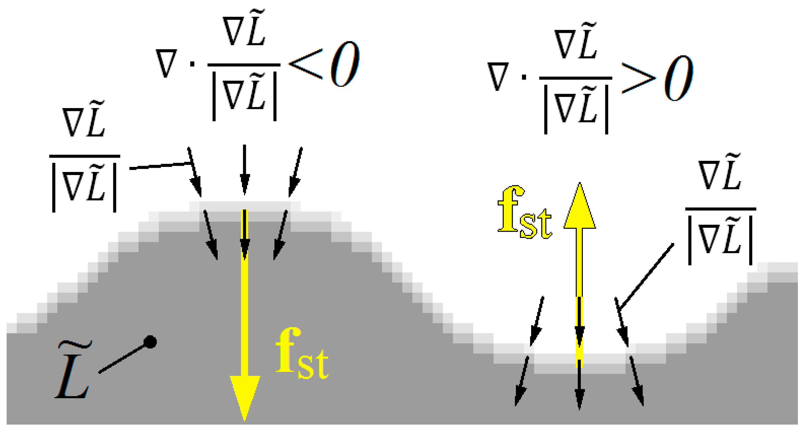
One of the most difficult problems is to calculate the volumetric equivalents of forces acting on a free surface. The surface tension force acts along the normal to the surface, and its magnitude will depend on the sign and magnitude of the surface curvature of. When using the Eulerian grid, the VOF method of free surfaces approximation and the liquid–vacuum boundary can become “blurred”, the representation of surface forces in the form of their volumetric equivalents is applied [24]. In this case, the magnitude and sign of the surface tension force will be determined through the divergence of the vector field of the surface normals. In this paper, the following expression was used to calculate the volumetric equivalent of the surface tension force [24]

$${\overrightarrow{f}}_{st}=\sigma ·\left(-\nabla ·\frac{\nabla \tilde{L}}{\left|\nabla \tilde{L}\right|}\right)·\nabla \tilde{L},$$

(12)

where σ is surface tension of the material, N/m; the scalar value equivalent to the curvature of the surface is indicated in parentheses; the last multiplier is the product of the normal vector $\frac{\nabla \tilde{L}}{\left|\nabla \tilde{L}\right|}$ on the modulus of the vector $\nabla \tilde{L}$, which in this case is the equivalent of a delta function having a nonzero value only near the free surface. Multiplying the normal by $\left|\nabla \tilde{L}\right|$ gives $\nabla \tilde{L}$. The tilde sign over L means that a “smoothed” scalar field L, obtained by the moving average method, is used in calculations. The use of a smoothed field makes it possible to reduce the influence of errors in estimation of normals and their divergence due to finite-difference digitization of the calculation area. Figure 2 graphically shows the values included in the expression (12).

The vapor recoil pressure was calculated as the saturated vapor pressure at the liquid surface in accordance with the Antoine’s equation. If the point x, y, z lies on the free surface of the liquid, the following function can be written as

$$p_{rec}=133\times {10}^{\mathrm{A}-\frac{\mathrm{B}}{T_{x,y,z}}},$$

(13)

where T_x,y,z is the temperature at the specific point. Then the volumetric equivalent of the vapor pressure force for points lying on this surface can be determined by the expression

$${\overrightarrow{f}}_{rec}={-\nabla p|}_{\left(x,y,z\right)\in \mathsf{\Gamma }}.$$

(14)

Assuming that ${\overrightarrow{f}}_{rec}$ is perpendicular to the free surface everywhere and is directed into the molten pool

$${\overrightarrow{f}}_{rec}=\left|\nabla p\right|\frac{\nabla \tilde{L}}{\left|\nabla \tilde{L}\right|}.$$

(15)

Based on the expressions (1–15), the finite difference method and the grid shown in Figure 1, the computer program was developed in the Microsoft Visual Studio environment. The program was used to simulate the process of electron beam metal wire deposition method with the formulation of the problem described below.

3. Computational Experiment Description, Verification of the Results, and Discussion

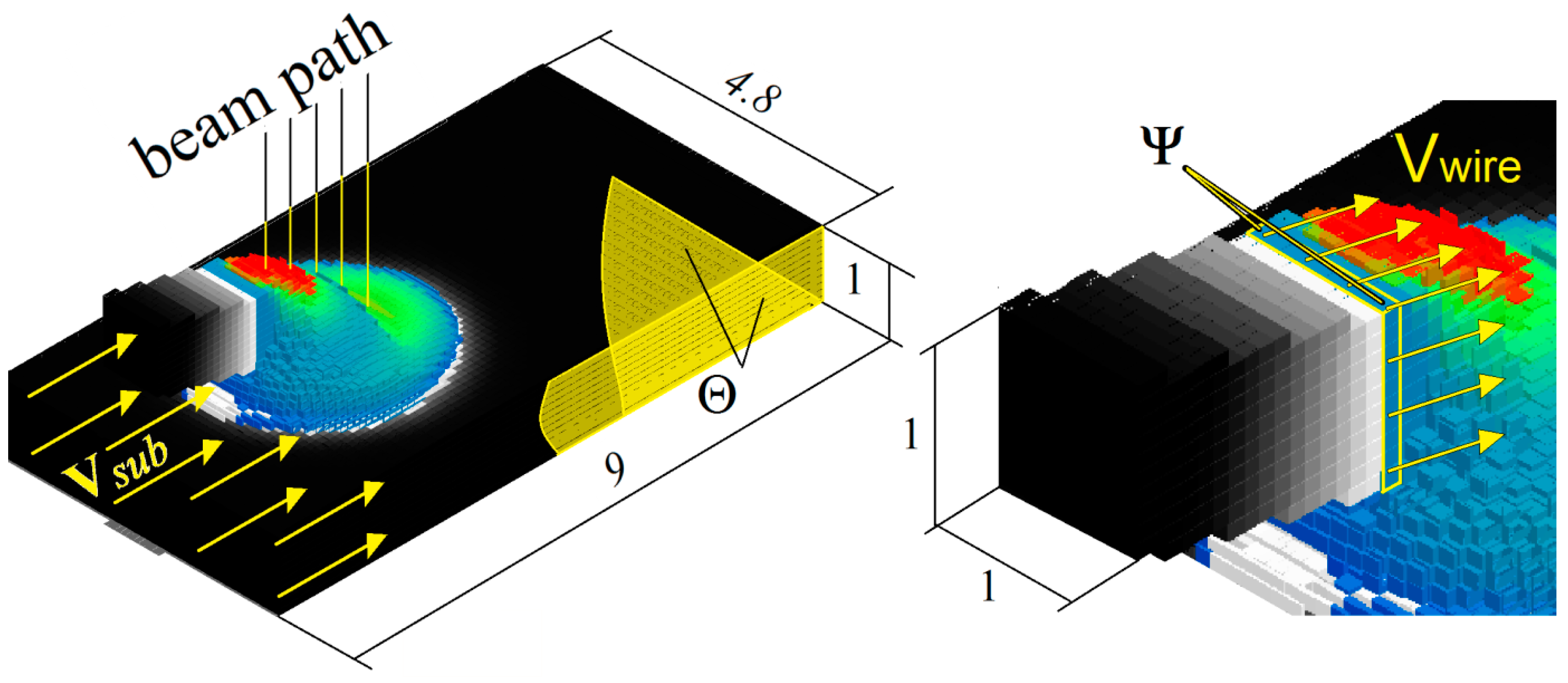
Figure 3 shows a graphical interpretation of the computational domain. The wire is presented in the form of a rectangular cross-section profile (position 1), at the end of which, in the region ψ, boundary conditions of the first-type for temperature and flow rate are set

$$\begin{gathered} {T|}_{\left(x,y,z\right)\in \mathsf{\Psi }}=2000 °\mathrm{C}, \\ {v_{\mathrm{wire}.\mathrm{x}}|}_{\left(x,y,z\right)\in \mathsf{\Psi }}=38.5 \mathrm{m}\mathrm{m}/\mathrm{s},{v_{\mathrm{wire}.\mathrm{z}}|}_{\left(x,y,z\right)\in \mathsf{\Psi }}=11 \mathrm{m}\mathrm{m}/\mathrm{s}. \end{gathered}$$

(16)

The boundary condition type and temperature values were chosen to ensure the continuous flow of the metal from the wire. Such approach allows investigating beam oscillation contribution to the metal transfer on the formed deposited layer. For this reason, fluctuations in the metal flow rate at the end of the wire, which in practice are associated with changes in its temperature over time, were not considered. The direction of the velocity vector coincides with the direction of the wire feed, and the value of the velocity modulus (v_wire = 40 mm/s) is selected in accordance with the experimental data.

To reduce the calculation time, the substrate is presented as an element of the calculation area having rectangular cross-section with dimensions of 9 × 4.8 × 1 mm. To exclude through-melting of the substrate on its lower and lateral planes (see the area Θ in Figure 3), the first-type boundary condition for temperature is set

$${T|}_{\left(x,y,z\right)\in \mathsf{\Theta }}=20 °\mathrm{C}.$$

(17)

The substrate moved with a constant velocity v_sub = 10 mm/s in respect to the beam. The substrate motion in the solid state is modeled in the same way as metal flow, but all elements of the substrate move in the same direction and at a constant speed. This is taken into account when solving Equations (8) and (9).

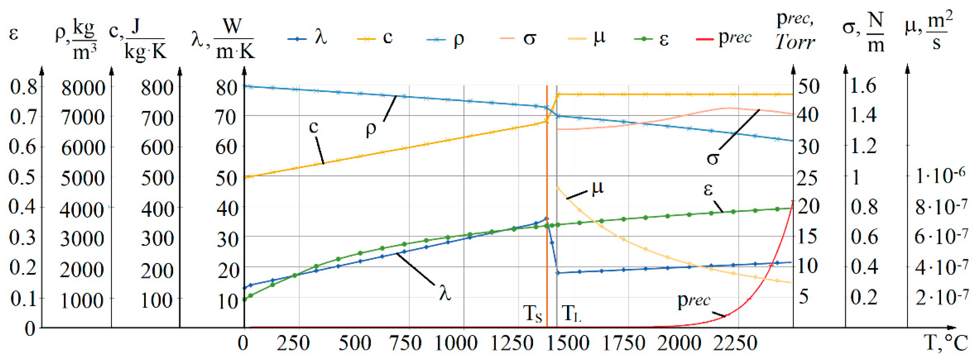
Figure 4 shows the temperature dependences of the properties for stainless steel 316L used in modeling and taken from the literature [25,26,27,28]. To account for these dependencies, the iterative method was not used in the model: the parameter value for the control volume at the current time step was taken for the temperature calculated at the previous time step.

Figure 5 graphically shows the results of modeling the surfacing process with electron beam longitudinal oscillation. The oscillation amplitude of the electron beam was 1.5 mm, and the frequency equaled to 100 Hz. The beam was positioned on the wire and moved continuously away from it and at a constant speed along the y axis (its trajectory is shown in Figure 3). After moving away from the wire by 1.5 mm, the beam instantly returned to its original position. The volumetric heat source was set by a uniform distribution function

$$q_v=\{\begin{array}{cc}0,& z<z_{\mathrm{sur}}\\ \frac{1}{\pi ·r_{\mathrm{eff}}{}^2}{P}_{\mathrm{b}}\frac{1}{h},& z=z_{\mathrm{sur}}\\ 0,& z>z_{\mathrm{sur}}\end{array}$$

(18)

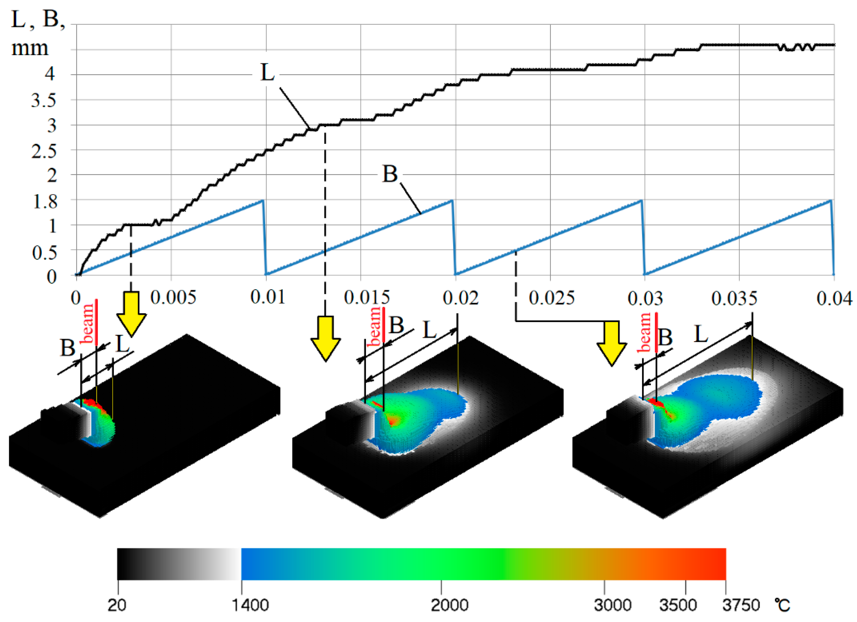
where P_b = 1000 W is electron beam power, r_eff = 0.4 mm is electron beam radius. The source in the form of a volume-distributed function is preferable at this stage, because it can proceed further to the consideration of microscale processes, namely, the study of absorption and backscattering of electrons [21]. Figure 5 shows the time dependences of electron beam position B and crystallization front L relative to the wire.

It can be seen from Figure 5 that molten pool length, characterized by L value, increases with a periodicity corresponding to the beam oscillations. However, there is some delay (0.005 s) due to the inertia of the metal movement, primarily related to viscosity. It is also seen that the rate of elongation of the molten pool is gradually decreasing, and thus, after a certain time, a quasi-stationary transfer mode should occur: the metal will periodically move from the wire along the pool, but the pool will maintain an almost unchanged length. Excessively high temperatures in the location of the electron beam here (Figure 5) and below calculated in the model are associated with not taking into consideration the latent heat of vaporization of the metal at this stage of research.

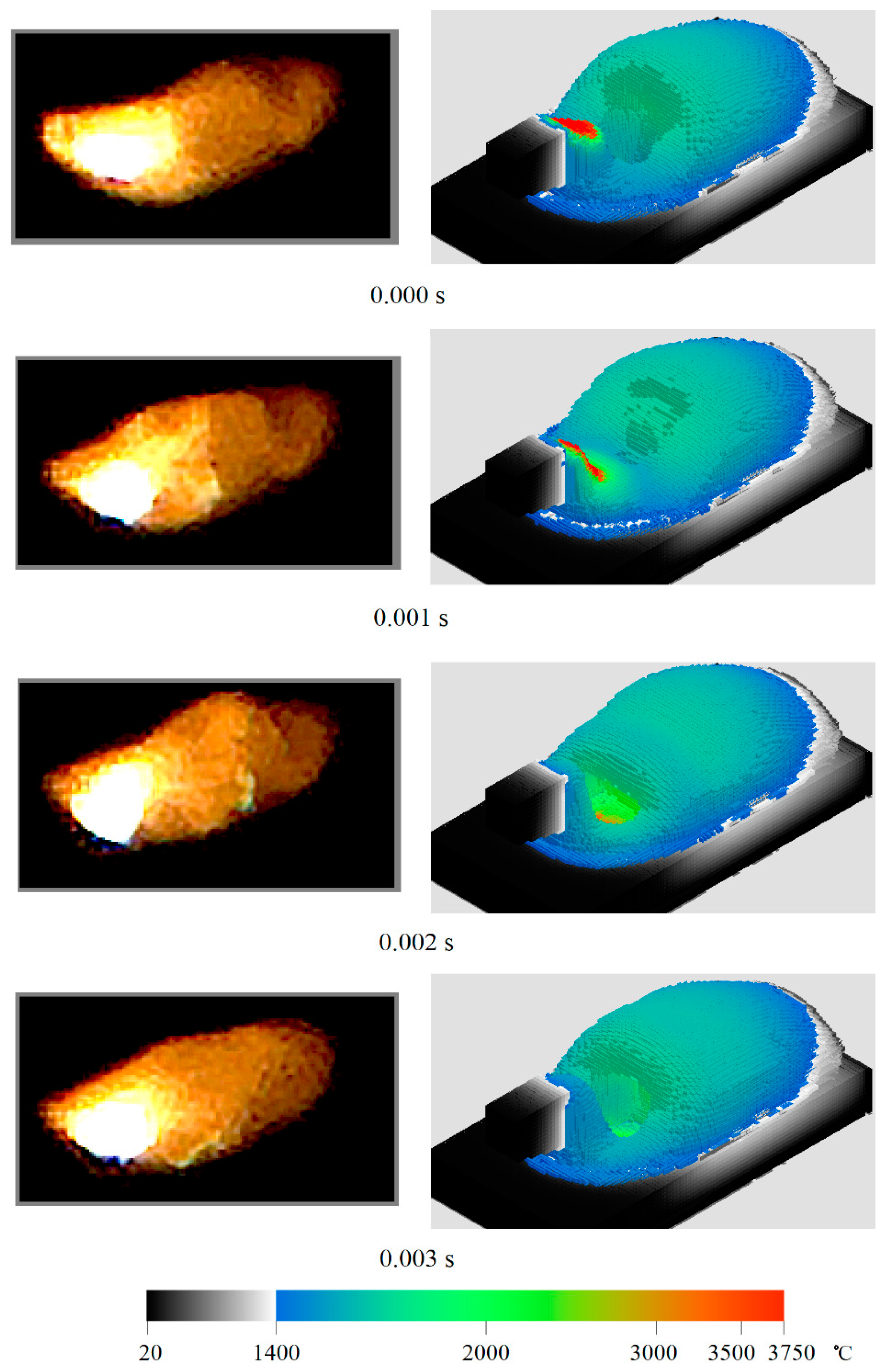
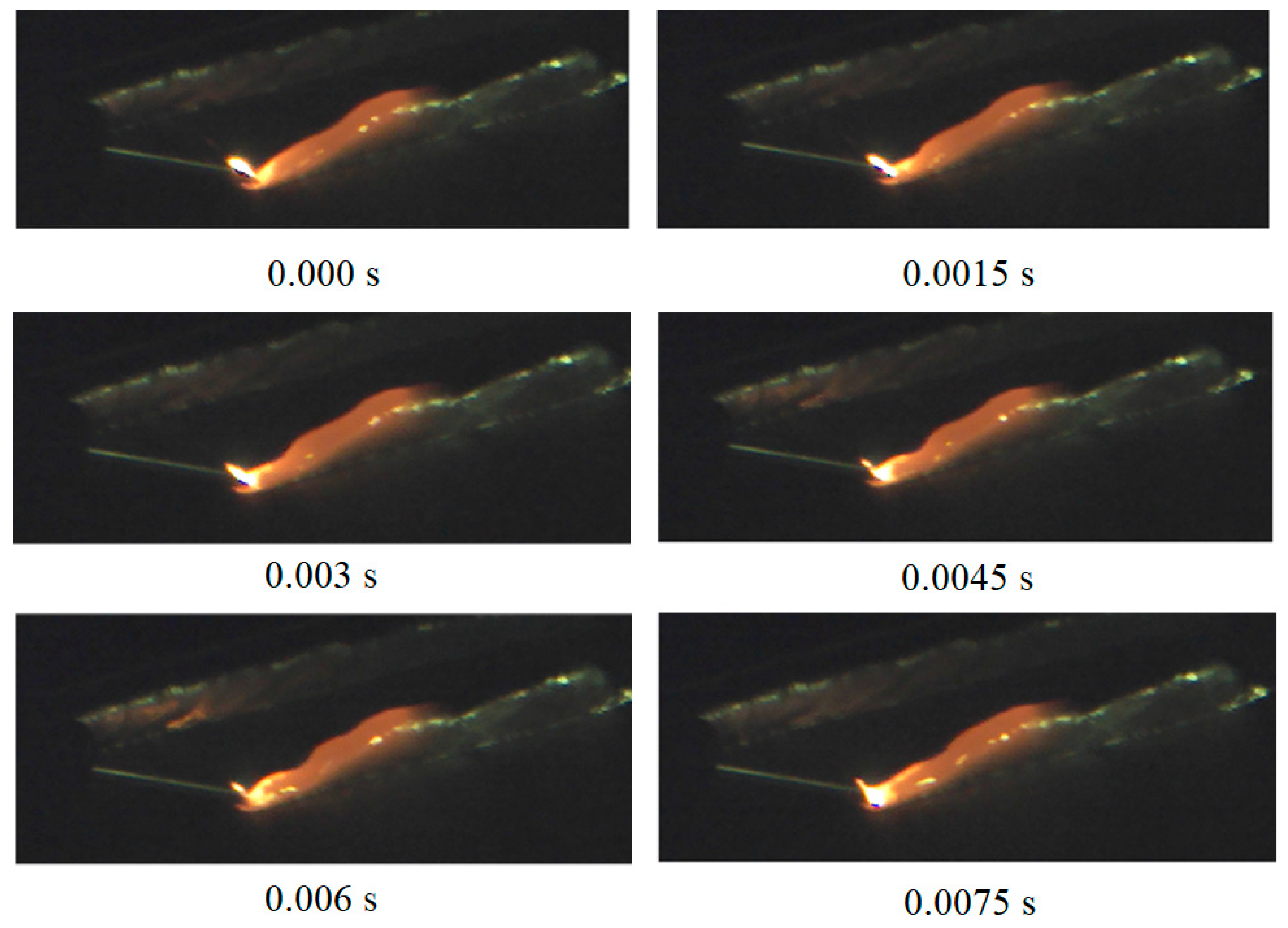
Figure 6 shows the images from the high-speed video recording obtained using the high-speed camera IDT OS Os7-S3 [29] with a shooting frequency of 4000 frames per second. The oscillation frequency of the beam with a power of P_b = 800 W was also 100 Hz, while its amplitude was equal to 1 mm.

The above frames illustrate that, in the process of metal transfer, there are fluctuations in the height of the pool, and the waves arising on the free surface move in the direction from the wire to the product. The excitation of vibrations in a liquid metal leads to a layer-by-layer increase in the height of the deposited layer, which is also shown by the created mathematical model. The length of the pool during the transfer remains almost constant, which corresponds to a quasi-stationary transfer mode.

Obviously, the best method for verifying the proposed model was to compare the calculated temperature values with those obtained using specialized thermal imagers. However, since the beam oscillation with a frequency of 100 Hz is used, it determines the dynamic processes in the molten pool, and the use of industrial thermal imagers would not be informative (due to a significantly lower frame rate). The use of scientific near-infrared range (NIR) cameras is possible, however, due to the short exposure time, it will not provide a sufficient dynamic range. For these reasons, it is advisable to use high-speed visible-range cameras whose frame rate can reach tens of thousands of frames per second.

Therefore, to verify the developed model, the images obtained with the camera at the beginning of the surfacing process were compared with the dimensions and cross-section shape of the liquid pool in the Y0Z plane calculated using the model (Figure 7).

The left part of the figure presents video images captured during beam oscillation with a frequency of 100 Hz, while on the right part the results of computational experiments for the corresponding time points are depicted. The moment of time t = 0.000 s corresponds to the transition of the beam from the pool to the wire: in the back of the pool there is still the front of the wave created earlier by the electron beam located there. Then it begins to move from the wire to the pool, heating and vaporizing the metal, to create an area of overpressure near the supplied wire. As a result, the rise of the melt in this region is initiated at time t = 0.001 s. Then, under the action of the vapor recoil pressure created by the beam moving towards the pool, the metal wave shifts towards the ‘tail’ of the pool (t = 0.002 s), which leads to an intensification of the directional transfer and elongation of the pool, noticeable already at t = 0.003 s. The full cycle of beam movement is repeated after 0.01 s.

This example shows that at the initial stage of the wire material melting, the model provides a result that is qualitatively consistent with experimental data: when the beam oscillates at a frequency of 100 Hz, ‘waves’ are formed in the molten pool moving from the wire to the back of the pool.

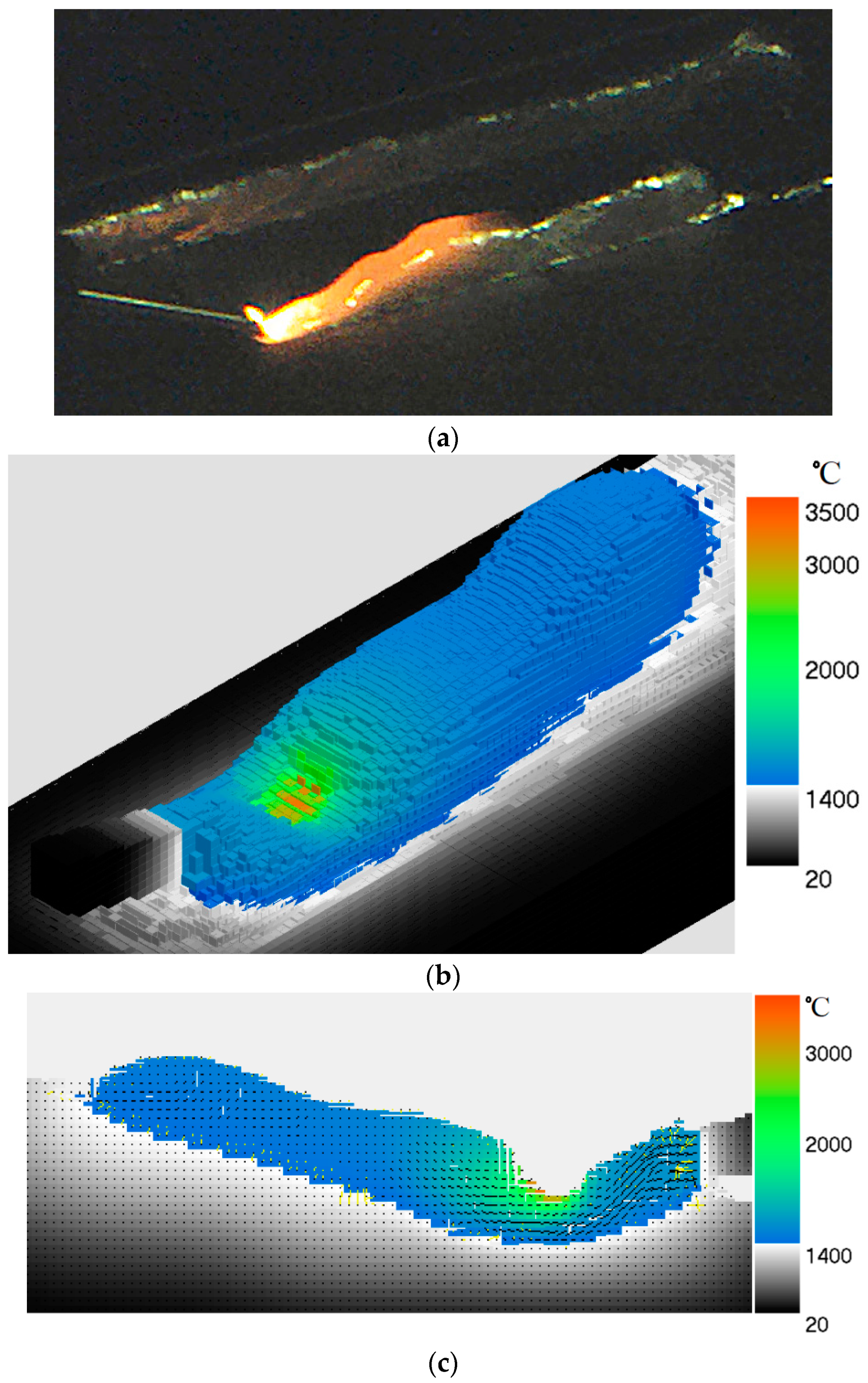
However, the study of further development of the surfacing process with periodic beam deflection according to the saw-tooth law is of the greatest interest. In this mode, a narrower and longer pool will be formed (see Figure 6), and the deposited layers, obviously, will differ in a large height-to-width ratio in comparison with depositing without longitudinal oscillation. The results of studying the process of forming such a deposited layer are shown in Figure 8.

The periodic continuous movement of the beam from the wire along the deposited layer with an ‘instantaneous’ deviation to the initial position (to the wire) influences the liquid pool similar to the action of a mechanical jet propulsion. It is based on the message of additional acceleration of the liquid due to the recoil pressure of metal vapor created by an electron beam. Due to the periodic nature of the impact, not only one wave appears at the liquid–vacuum interface, but a sequence of waves propagating in the melt, which are clearly visible in Figure 8a. The pool not only stretches in the direction from the wire, but also overlaps the previously formed crystallized layer. This can be explained by the fact that additional velocity is communicated to the melt. It suggests the conclusion that the molten metal moves along the inclined surface of the previously formed layer in the direction from bottom to top, which is clearly shown by the results of computational experiments (Figure 8b,c). The black segments in Figure 8c display the magnitude and direction of the metal velocity vectors. The maximum values of the flow rate are observed in the feed area of the filler material. It is also seen that the velocity vectors lengthen at the surface of the pool under the influence of vapor pressure generated by the electron beam. Since liquid metal has been considered as an incompressible liquid, the velocity field will be solenoidal during the movement and interaction of moving waves with solid walls and areas where vapor pressure acts (in the area of the beam action). Moreover, closed currents will occur.

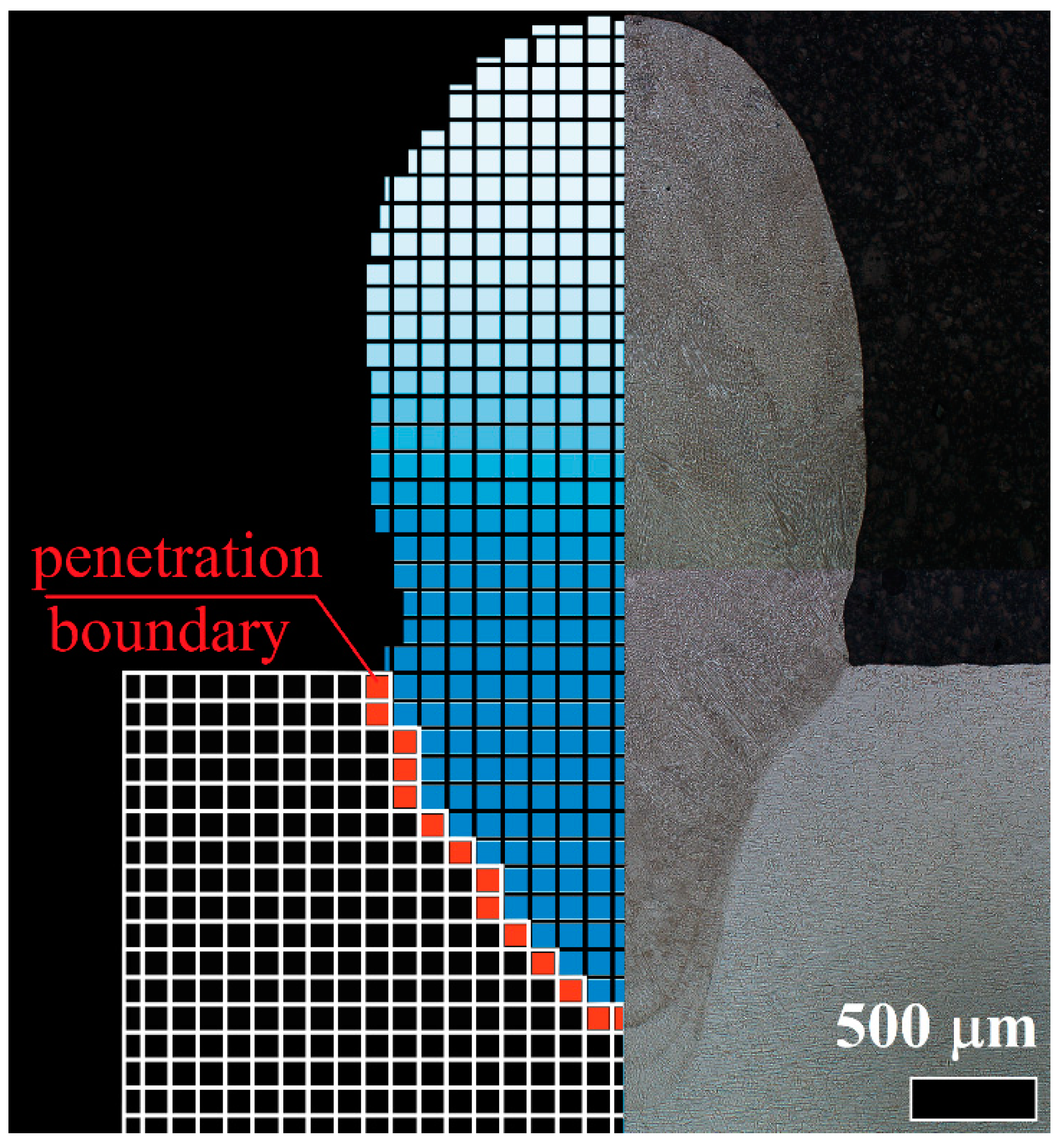
The comparison of the transverse macrosection of deposited layer at the same parameters (beam power P_b is equal to 800 W, oscillation frequency is 100 Hz, oscillation amplitude is 1 mm) was carried out; its results are illustrated in Figure 9. It revealed a slight deviation of the penetration area from the experimental one (within 12%), as well as the shape of the layer, which can be observed in the Figure 9. The main parameters, such as the height and average width of the layer, differ slightly (the deviation of the maximum height is less than 5%, and the average deviation of the average width of the layer is about 10%).

The conducted research shows the relevance of the model application to analyze the processes of dynamic impact on the molten pool using spatial oscillations of various types.

The temporal and spatial characteristics of molten pool free surface oscillations obtained in the simulation are in good agreement with the experimental data. In addition, the model reproduces the phenomenon of directional metal transfer to the tail of the molten pool. This makes it possible to substantiate the applicability for studying the processes of dynamic action on the molten pool at high frequencies of beam oscillations (about 100 Hz), which is important not only for wire-based additive manufacturing processes, but also for technologies of electron beam melting, welding, cutting, surface modification, etc.

4. Conclusions

1. A mathematical model of heat and mass transfer has been proposed. The temperature dependences of the thermophysical characteristics of the medium, as well as viscosity and surface tension which are suitable for analyzing the processes of metal flow during the deposition process—including the processes with electron beam spatial oscillation—have been taken into account.

2. The results of computational experiments have shown that when an electron beam oscillates along the direction of surfacing according to a saw-tooth law with a frequency close to 100 Hz, a mode in which the metal acquires an additional velocity in the direction from the wire to the deposited layer has been achieved.

3. By comparing the simulation results with video images obtained using a high-speed camera, the model was verified. As a result, the model adequately reflects the transfer processes. During both computational and laboratory experiments, the simultaneous existence of several waves on the molten metal–vacuum interface was revealed, and the phenomenon of metal lifting onto previously deposited crystallized layers was also established.

4. A simulation of depositing a layer with a height of about 2.5 mm (from the substrate plane) and an average width of about 2 mm with an electron beam oscillation was carried out; a satisfactory coincidence of the shape and size of the deposited layer was achieved. It also confirms the relevance of using the model to study the processes of the dynamic effect of electron beams on molten materials when using oscillation.