Strain-Gradient Crystal Plasticity Finite Element Modeling of Slip Band Formation in α-Zirconium

Abstract

Two methods for the determination of geometrically necessary dislocation (GND) densities are implemented in a lower-order strain-gradient crystal plasticity finite element model. The equations are implemented in user material (UMAT) subroutines. Method I has a direct and unique solution for the density of GNDs, while Method II has unlimited solutions, where an optimization technique is used to determine GND densities. The performance of each method for capturing the formation of slip bands based on the calculated GND maps is critically analyzed. First, the model parameters are identified using single crystal simulations. This is followed by importing the as-measured microstructure for a deformed α-zirconium specimen into the finite element solver to compare the numerical results obtained from the models to those measured experimentally using the high angular resolution electron backscatter diffraction technique. It is shown that both methods are capable of modeling the formation of slip bands that are parallel to those observed experimentally. Formation of such bands is observed in both GND maps and plastic shear strain maps without pre-determining the slip band domain. Further, there is a negligible difference between the calculated grain-scale stresses and elastic lattice rotations from the two methods, where the modeling results are close to the measured ones. However, the magnitudes and distributions of calculated GND densities from the two methods are very different.

1. Introduction

Crystal plasticity is a class of constitutive equations that can be used to describe deformation mechanisms of polycrystalline materials at the grain scale [1,2,3]. It has been used in many studies to understand the evolution of heterogeneous deformation fields within individual grains in “real” time scales [4,5,6,7]. A significant number of crystal plasticity studies have focused on modeling deformation via slip, which is controlled by the movement of dislocations on a particular plane known as the slip plane and in a particular direction known as the slip direction. The strength of the obstacles interacting with dislocations determines the resistance of a slip system to the movement of the dislocations and the consequent material hardening. These obstacles can be categorized into short-range and long-range barriers [8]. The primary short-range obstacles are generally assumed to be the other dislocations that intersect the slip plane. The long-range obstacles may include the elastic stress field induced by far field dislocations or grain boundaries. It is generally assumed that the long-range obstacles are affected by the density of the geometrically necessary dislocations (GNDs), while the evolution of both statistically stored dislocations (SSDs) and GNDs during crystallographic slip equally increase the short-range interactions [9,10]. When conventional crystal plasticity models are used, the difference between these two obstacles is generally ignored and the critical resolved shear stress (CRSS) for the movement of the dislocations does not depend on the deformation state in the neighboring points. However, the plastic response of a polycrystal depends on both the local state of deformation and the gradients of the plastic strain. Incorporation of the plastic strain gradient in crystal plasticity constitutive equations makes the model response dependent on the neighboring elements—this is generally investigated in the non-local crystal plasticity approach [11,12,13,14,15]. The strain-gradient plasticity theories are formulated in two different forms, i.e., the lower-order and higher-order approach [16]. In the lower-order approach [17,18,19], the plastic strain gradient terms are only incorporated in the hardening laws. However, in the higher-order approach, the equilibrium equations are also adjusted [20,21,22,23]. This paper focuses on examining the methods available in the literature for calculating GND densities in the lower-order crystal plasticity framework by providing a direct comparison between the results of each method to those measured experimentally.

GND densities are inherently linked to the lattice curvature and can be determined using the gradients of plastic strain [24]. The derivation of the dislocation densities from the “curl” of the deformation gradient in the Nye equation has been accompanied with inconsistencies in the literature, some of which have been reported by Das et al. [25]. Generally, two methods are used in the literature for extracting GNDs using Nye equations. In the first method, the contribution of each slip system, e.g., α, to GND density is assumed to be proportional to the plastic shear accommodated on the same slip system α. Hence, the number of linear equations that should be solved is equal to the number of unknowns, i.e., GNDs on each slip system α. This is called the direct method, where the density of GNDs on each slip system is determined unambiguously. The direct method was initially proposed by Dai [26] and was subsequently implemented in crystal plasticity finite element (CPFE) models [10,18,27,28,29]. In the second method, the cumulative contribution of plastic shears on all slip systems to the total GND densities on all slip systems is assumed to be proportional to the Nye tensor. This usually results in an under-determined system of equations where the number of unknowns is more than the number of equations. Two main approaches are suggested for determining the unknowns. In the first approach, known as L¹, a solution is found by minimizing the dislocation line energy. In the second approach, known as L², a solution is found by minimizing the sum of the squares of the dislocation densities [30]. Das et al. showed that the use of the L² method leads to a solution where dislocation densities are evenly distributed on all slip systems, while the use of the L¹ method leads to capturing some variations of GNDs between the slip systems [25]. Negligible difference was found between the magnitudes of the total dislocation densities obtained from the two minimization approaches. The L² minimization approach has been widely used in the CPFE models [31,32,33,34]. In contrast to the direct method, which provides a unique solution for the GND density on each slip system, both minimization approaches lead to non-unique solutions. Therefore, an investigation is required to compare the magnitudes and distributions of the obtained GND densities from these two methods.

The measurement of internal stress and dislocation densities helps validate dislocation-based crystal plasticity models. Diffraction-based experimental methods are mainly used for measuring internal lattice strains [35,36,37,38] and localized stress fields [38,39] as well as the density of dislocations [40]. For example, the dislocation densities in the vicinity of slip bands in HCP polycrystals were measured using micro X-ray diffraction [41]. Although a three-dimensional view of the dislocation densities is provided, only a few grains can be studied in this technique. A high angular resolution electron back scatter diffraction (HR-EBSD) technique can be used to measure “relative” elastic strains and rotations and “absolute” GND densities for many grains, yet close to the sample surface. Diffraction patterns are collected and then cross correlated using a reference pattern. The deformation gradient tensor is then calculated and used to determine the relative elastic strain tensor [42,43,44,45] and GND densities using the Nye tensor [46]. Many studies have used HR-EBSD to compare the numerically obtained GND densities from CPFE models to the measured ones [33,47,48,49].

The objectives of this paper are to compare the GND densities calculated using the direct method to those obtained from the minimization-based method and investigate the capability of the GND-based CPFE models in capturing the formation of slip bands in an α-zirconium polycrystal. Hence, the direct and the minimization-based methods for calculating GND densities are formulated and implemented in a lower-order strain-gradient CPFE model. After calibrating single crystal parameters, the evolution of GND and SSD densities predicted using each method is studied in detail using single crystal FE models. The capability of the developed non-local models in capturing the experimentally observed slip bands of a deformed polycrystalline α-zirconium is subsequently investigated. This is followed by comparing the results of the models for GND densities, stresses, and elastic rotations to those measured via HR-EBSD.

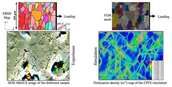
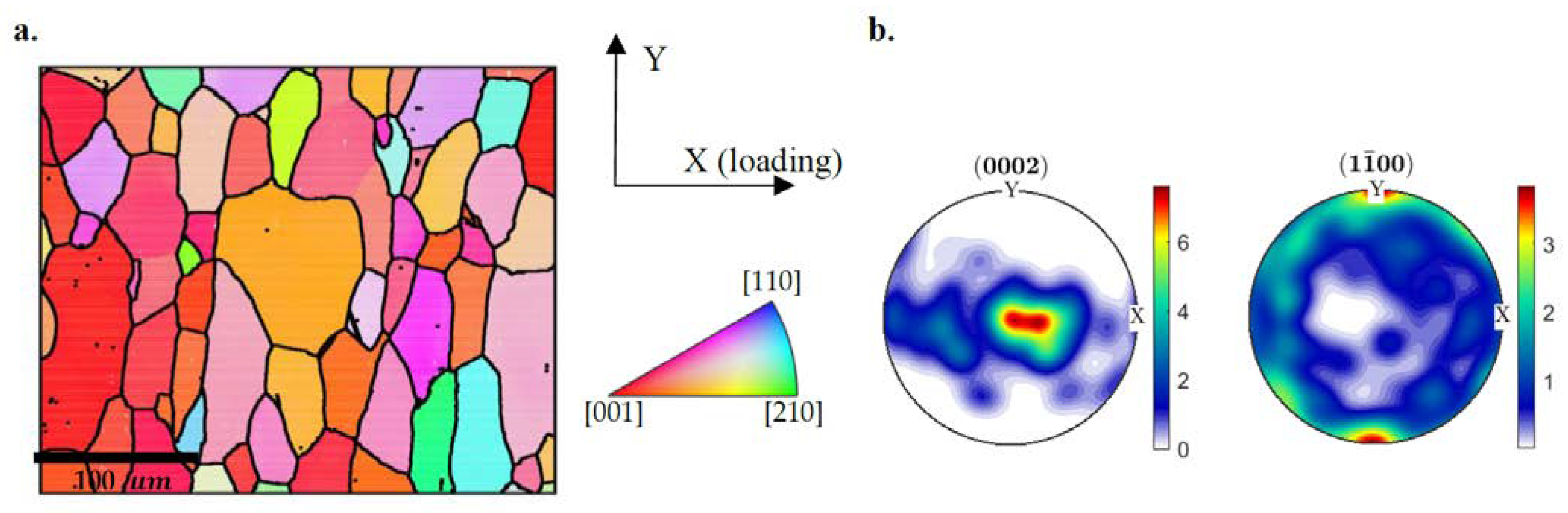
2. Sample Preparation and Experimental Set Up

Blocks of α-zirconium material were firstly annealed at 700 °C and then air cooled to relieve residual stresses as much as possible. A dog bone sample was subsequently made with a gauge length of 20 mm. The sample was mechanically polished down to 4000 grit, followed by polishing in a 50 nm colloidal silica suspension and electropolishing in a −30 °C solution of 90% methanol and 10% perchloric acid for 60 s at 25 V. The cross section of the sample after polishing was measured to be 0.5 × 0.5 mm².

The sample was uniaxially deformed at room temperature under strain control to a tensile strain of 1.2% using a strain rate of 2.6 × 10⁻⁵ s⁻¹. The EBSD measurement was performed in a Zeiss MERLIN field emission gun scanning electron microscope (FEG-SEM) with 20 keV beam energy, 15 nA probe current, and at the working distance of 18 mm. Diffraction patterns were collected every 0.5 $\mathsf{\mu }\mathrm{m}$ using a Bruker high resolution EBSD detector. Following the method developed by Wilkinson et al. [42], elastic strain and lattice rotations were calculated by cross correlating the collected 800 × 800 pixels Kikuchi patterns [50]. An EBSD map of the deformed sample with the coordinate system used is shown in Figure 1a. As shown, the X-axis coincides with the loading direction, the Z-axis is along the electron beam direction and sample thickness, and the Y-axis is defined by the cross product of the other two axes. In addition, as shown in Figure 1b, the c-axis of the HCP crystals is oriented towards the z-axis with a little spread towards the x-axis. Since the specimen was only deformed to 1.2% and the c-axis of most of the crystals is perpendicular to the loading direction, deformation twinning was not active in this experiment. No twin was observed in the EBSD and the ARGUS images taken from sample after deformation. As such, the effects of twinning are ignored in all mathematical formulation and CPFE modeling.

3. Crystal Plasticity Formulation and Input Model

In this section the constitutive equations implemented for calculating GND densities using both the direct and minimization-based methods are described. Here, the direct and minimization-based methods are called “Method I” and “Method II”, respectively. These equations are implemented in a User MATerial (UMAT) subroutine originally developed by Abdolvand et al. [51] and recently updated by Sedaghat and Abdolvand [47]. After describing the implemented constitutive equations, the steps followed to prepare the FE input model are presented.

3.1. Crystal Plasticity Constitutive Equations

The total deformation gradient ($\mathit{F}$) can be decomposed to the elastic (${\mathit{F}}^{\mathit{e}})$ and plastic (${\mathit{F}}^{\mathit{p}}$) parts:

$$\mathit{F}={\mathit{F}}^{\mathit{e}}{\mathit{F}}^{\mathit{p}}$$

(1)

The total velocity gradient tensor ($\mathit{L}$) in the current configuration can be divided into the elastic (${\mathit{L}}^{\mathit{e}}$) and plastic (${\mathit{L}}^{\mathit{p}}$) parts as:

$$\mathit{L}=\dot{\mathit{F}}{\mathit{F}}^{-\mathbf{1}}={\dot{\mathit{F}}}^{\mathit{e}}{\mathit{F}}^{\mathit{e}-\mathbf{1}}+{\mathit{F}}^{\mathit{e}}{\dot{\mathit{F}}}^{\mathit{p}}{\mathit{F}}^{\mathit{p}-\mathbf{1}}{\mathit{F}}^{\mathit{e}-\mathbf{1}}={\mathit{L}}^{\mathit{e}}+{\mathit{L}}^{\mathit{p}}$$

(2)

The total velocity gradient tensor can be divided into its symmetric part, i.e., deformation rate tensors $\left({\mathit{D}}^e,{\mathit{D}}^p\right)$, and asymmetric part, i.e., spin tensors$\left({\mathit{\Omega }}^e,{\mathit{\Omega }}^p\right)$. The plastic part of the velocity gradient tensor is calculated using the following equation [52]:

$${\mathit{L}}^{\mathit{p}}={\mathit{D}}^p+{\mathit{\Omega }}^p={\displaystyle \sum }_{\alpha =1}^N{\dot{\gamma }}^{\alpha }{\overrightarrow{m}}^{\alpha }\otimes {\overrightarrow{n}}^{\alpha }$$

(3)

where ${\overrightarrow{m}}^{\alpha }$, ${\overrightarrow{n}}^{\alpha }$, and ${\dot{\gamma }}^{\alpha }$ respectively represent the slip direction, the slip plane normal, and the shear rate on the $\alpha$th slip system for the $N$ number of active slip systems. ${\overrightarrow{m}}^{\alpha }\otimes {\overrightarrow{n}}^{\alpha }$ is known as the Schmid tensor of the slip system $\alpha$. The shear rate on the slip system $\alpha$ is calculated based on the resolved shear stress (${\tau }^{\alpha }$) acting on the same slip system [52]:

$${\dot{\gamma }}^{\alpha }={\dot{\gamma }}_0^{\alpha }\mathrm{sign}\left(\frac{{\tau }^{\alpha }}{g^{\alpha }}\right){\left|\frac{{\tau }^{\alpha }}{g^{\alpha }}\right|}^n$$

(4)

where ${\dot{\gamma }}_0$ is a reference shear strain rate, $n$ represents the sensitivity of the material to a strain rate, and $g^{\alpha }$ is the CRSS of the slip system $\alpha$. The resolved shear stress acting on the slip system $\alpha$ is proportional to Kirchhoff stress ($\mathit{\psi }$) through the following equation [53]:

$${\tau }^{\alpha }={\mathit{P}}^{\mathit{\alpha }}:\mathit{\psi }$$

(5)

where ${\mathit{P}}^{\mathit{\alpha }}$ is the symmetric part of the Schmid tensor. The Jaumann rate of the Kirchhoff stress tensor ($\check{\mathit{\psi }}$) is related to the elastic part of the deformation rate tensor (${\mathit{D}}^{\mathit{e}}$) and the elastic stiffness tensor ($ℂ$) of the HCP crystal after rotation to the deformed configuration as:

$$\check{\mathit{\psi }}=ℂ:{\mathit{D}}^e$$

(6)

The elastic modulus of zirconium HCP crystals used in this study is the one determined by Fisher and Renken [54]: C₁₁ = 143.5 GPa, C₃₃ = 164.9 GPa, C₁₂ = 72.5 GPa, C₁₃ = 65.4 GPa, and C₄₄ = 32.1 GPa. The objective rate of Kirchhoff stress, in Equation (6), is defined as:

$$\check{\mathit{\psi }}=\dot{\mathit{\psi }}-{\mathit{\Omega }}^{\mathit{e}}\mathit{\psi }+\mathit{\psi }{\mathit{\Omega }}^{\mathit{e}}$$

(7)

The strength of each slip system ($g^{\alpha }$) in Equation (4) follows a dislocation-based hardening law [10,11,12,27]:

$$g^{\alpha }=g_{*,0}^{\alpha }+\frac{H^{\alpha }}{\sqrt{D}}+\xi G{b}^{\alpha }\sqrt{{\displaystyle \sum }_{\beta =1}^N{q}^{\alpha \beta }\left({\rho }_{GND}^{\beta }+{\rho }_{SSD}^{\beta }\right)}=g_{*,0}^{\alpha }+\frac{H^{\alpha }}{\sqrt{D}}+\xi G{b}^{\alpha }\sqrt{{\rho }_T}$$

(8)

where $g^{\alpha }$ is the updated CRSS, $g_{*,0}^{\alpha }$ is the initial CRSS, $D$ is the equivalent grain diameter, $H^{\alpha }$ is the Hall-Petch parameter for slip system $\alpha$, $\xi$ is a material constant, $G$ is the shear modulus, $b^{\alpha }$ is the size of the Burgers vector for the slip system $\alpha$, and ${\rho }_{GND}^{\beta }$ and ${\rho }_{SSD}^{\beta }$ are the GND and SSD densities on the slip system $\beta$. A hardening matrix $q^{\alpha \beta }$ is introduced to consider the effects of self- and latent-hardening. For the sake of simplicity in deriving a solution, the term under the radical is called ${\rho }_T$. It is assumed that the GND and SSD densities have the same hardening matrix $q^{\alpha \beta }$. The shear modulus, G in Equation (8), is assumed to be the average value of C₄₄, C₅₅, and C₆₆ [55]. The material constant $\xi$ is assumed to be 0.5.

It is assumed that the evolution of SSD densities follows the equation below [10,56]:

$${\dot{\rho }}_{SSD}^{\alpha }=\frac{\left|{\dot{\gamma }}^{\alpha }\right|}{b^{\alpha }}\left(K^{\alpha }\sqrt{{\rho }_{SSD}^{\alpha }+{\rho }_{GND}^{\alpha }}-2y_c^{\alpha }{\rho }_{SSD}^{\alpha }\right)$$

(9)

where $K^{\alpha }$ is the dislocation accumulation constant and $y_c^{\alpha }$ is the dislocation annihilation length. The first term in the right-hand side of the Equation (9) is the dominant term at the early stages of plasticity, while with further loading, the effects of the second term will be non-negligible. In the following sub-sections, the two methods used for calculating GND densities are presented.

3.1.1. Method I

In the first method, the GND density of the slip system $\alpha$ is uniquely correlated with the resolved shear strain accumulated on the same system [26]:

$${\dot{\rho }}_{GND}^{\alpha }=\frac{{\dot{\gamma }}^{\alpha }}{b^{\alpha }}\left|Curl\left[{\overrightarrow{n}}_j^{\alpha }{\mathit{F}}_{ji}^p\right]\right|=\frac{{\dot{\gamma }}^{\alpha }}{b^{\alpha }}\left|{ϵ}_{ikq}\frac{\partial \left({\overrightarrow{n}}_j^{\alpha }{\mathit{F}}_{jq}^p\right)}{\partial x_k}\right|$$

(10)

where ${ϵ}_{ikq}$ is the permutation tensor. Hence, ${\rho }_{GND}^{\alpha }$ has a unique solution. For implementing Equations (8)–(10) into the UMAT, the time derivative of Equation (8) is firstly calculated and coupled with Equations (9) and (10) to solve for the increments of shear strains using the Newton‒Raphson iterative algorithm. The evolution of CRSS can be reformulated by taking the time derivative of Equation (8):

$${\dot{g}}^{\alpha }=\xi G{b}^{\alpha }\frac{{\dot{\rho }}_T}{2\sqrt{{\rho }_T}},\mathrm{where}{\dot{\rho }}_T={\displaystyle \sum }_{\beta =1}^N{q}^{\alpha \beta }\left({\dot{\rho }}_{GND}^{\beta }+{\dot{\rho }}_{SSD}^{\beta }\right)$$

(11)

By substituting Equations (9) and (10) into Equation (11) we have:

$${\dot{g}}^{\alpha }={\displaystyle \sum }_{\beta =1}^N\left[q^{\alpha \beta }\frac{\xi G{b}^{\alpha }}{2b^{\beta }\sqrt{{\rho }_T}}\left(\left|{ϵ}_{ikq}\frac{\partial \left({\overrightarrow{n}}_j^{\alpha }{\mathit{F}}_{jq}^p\right)}{\partial x_k}\right|+K^{\beta }\sqrt{{\rho }_{SSD}^{\beta }+{\rho }_{GND}^{\beta }}-2y_c^{\beta }{\rho }_{SSD}^{\beta }\right)\right]{\dot{\gamma }}^{\beta }$$

(12)

The complexity of implementation of this method in the UMAT subroutine is calculation of the gradient term, which was originally developed by Abdolvand [57].

3.1.2. Method II

In the second method, the density of GNDs on the slip system $\alpha$ is defined as [30]:

$${\left(curl\left({\mathit{F}}^{p^T}\right)\right)}^T={\displaystyle \sum }_{\alpha =1}^N\left({\rho }_{GND, s}^{\alpha } {\overrightarrow{b}}^{\alpha }\otimes {\overrightarrow{m}}^{\alpha }+{\rho }_{GND,et}^{\alpha } {\overrightarrow{b}}^{\alpha }\otimes {\overrightarrow{t}}^{\alpha }+{\rho }_{GND,en}^{\alpha } {\overrightarrow{b}}^{\alpha }\otimes {\overrightarrow{n}}^{\alpha }\right)$$

(13)

${\rho }_{GND}^{\alpha }$ for each slip system can be decomposed into three components, one for screw type dislocation ${\rho }_{GND, s}^{\alpha }$ and two edge type dislocations, ${\rho }_{GND,en}^{\alpha }$ and ${\rho }_{GND,et}^{\alpha }$ with $t^{\alpha }=m^{\alpha }\times n^{\alpha }$, respectively. In contrast to Method I, Method II has infinite solutions where a minimization scheme is usually used to find a solution. Equation (13) can be solved by minimizing the sum of the squares of GND densities [19]:

$$\left\{{\rho }_{GND}^{\alpha }\right\}=A^T{\left(A{A}^T\right)}^{-1}B$$

(14)

where $\left\{{\rho }_{GND}^{\alpha }\right\}$ is 3N $\times$ 1 column vector including the components of GND for slip system $\alpha$, $B$ is a 9 $\times$ 1 vector, containing the curl function components in Equation (13), and $A$ is a 9 $\times$ 3N matrix with the basis tensors of Equation (13). The time derivative of Equation (13) is determined as:

$${\left(curl\left({\dot{\mathit{F}}}^{p^T}\right)\right)}^T={\displaystyle \sum }_{\alpha =1}^N\left({\dot{\rho }}_{GND, s}^{\alpha } {\overrightarrow{b}}^{\alpha }\otimes {\overrightarrow{m}}^{\alpha }+{\dot{\rho }}_{GND,et}^{\alpha } {\overrightarrow{b}}^{\alpha }\otimes {\overrightarrow{t}}^{\alpha }+{\dot{\rho }}_{GND,en}^{\alpha } {\overrightarrow{b}}^{\alpha }\otimes {\overrightarrow{n}}^{\alpha }\right)$$

(15)

By substituting Equations (15) and (9) into Equation (11), we have:

$${\dot{g}}^{\alpha }={\displaystyle \sum }_{\beta =1}^N\frac{q^{\alpha \beta }\xi G{b}^{\alpha }\left(K^{\beta }\sqrt{{\rho }_{SSD}^{\beta }+{\rho }_{GND}^{\beta }}-2y_c^{\beta }{\rho }_{SSD}^{\beta }\right)}{2b^{\beta }\sqrt{{\rho }_T}}.\left|{\dot{\gamma }}^{\beta }\right|+{\displaystyle \sum }_{\beta =1}^N\frac{q^{\alpha \beta }\xi G{b}^{\alpha }\left({\dot{\rho }}_{GND}^{\beta }\right)}{2b^{\beta }\sqrt{{\rho }_T}}$$

(16)

Similar to Method I, the first term in the right-hand side of Equation (16) shows an explicit correlation between the shear strain rate ${\dot{\gamma }}^{\beta }$ and ${\dot{g}}^{\alpha }$, but the second term represents the effects of GND evolution rate on ${\dot{g}}^{\alpha }$. Therefore, both GND density and the rate of GND density evolution should be determined in Method II. Further, a minimization approach must be followed to determine the two tensors. Accordingly, the implementation of Method II is relatively more complicated and computationally costly compared to Method I. Here, the method originally developed by Abdolvand [57] was adopted to calculate the curl of ${\mathit{F}}^{\mathit{p}}$, which was subsequently implemented in the UMAT as described in [47].

The single crystal parameters used for HCP zirconium for each method are provided in

Table 1. Single crystal parameters used in the hardening law for HCP zirconium from Sedaghat and Abdolvand [47].

		Prism	Basal	Pyramidal
n		20	20	20
${\dot{\gamma }}_0^{\alpha } \left(S^{-1}\right)$		3.5 × 10−4	3.5 × 10−4	1.0 × 10−4
$q^{ss}$(self)		1	1	1
$q^{st}$(t = prism)		1	1	0
$q^{st}$(t = basal)		1	1	0
$q^{st}$(t = pyramidal)		0	0	1
Burgers vector (nm)		0.323	0.323	0.608
$H^{\alpha } \left(MPa \sqrt{m}\right)$		0.109	0.146	0.292
$g_{*,0}^{\alpha } \left(MPa\right)$		95	135	266
MI	$K^{\alpha }$	0.07	0.07	0.30
	$y_c^{\alpha } \left(\mathrm{nm}\right)$	5	5	10
MII	$K^{\alpha }$	0.05	0.05	0.30
	$y_c^{\alpha } \left(\mathrm{nm}\right)$	5	5	10

. The single crystal parameters for the Method II model were calibrated using a comprehensive data set measured in a series of in-situ neutron diffraction experiments conducted on HCP zirconium polycrystals [58]. Measured macroscopic stress-strain curves, lattice strains, and texture development were used to calibrate the model parameters as explained in [47]. The model parameters for Method I are calibrated such that they reproduce identical stress-strain curves to those from the model with Method II. The initial SSD density is set at 10¹⁰ m⁻² for both methods. The effect of twinning is ignored in the simulations since no twin was observed in the experiment. Here, only the single crystal parameters for Method I require calibration. The process of calibration is discussed in Section 4.1.

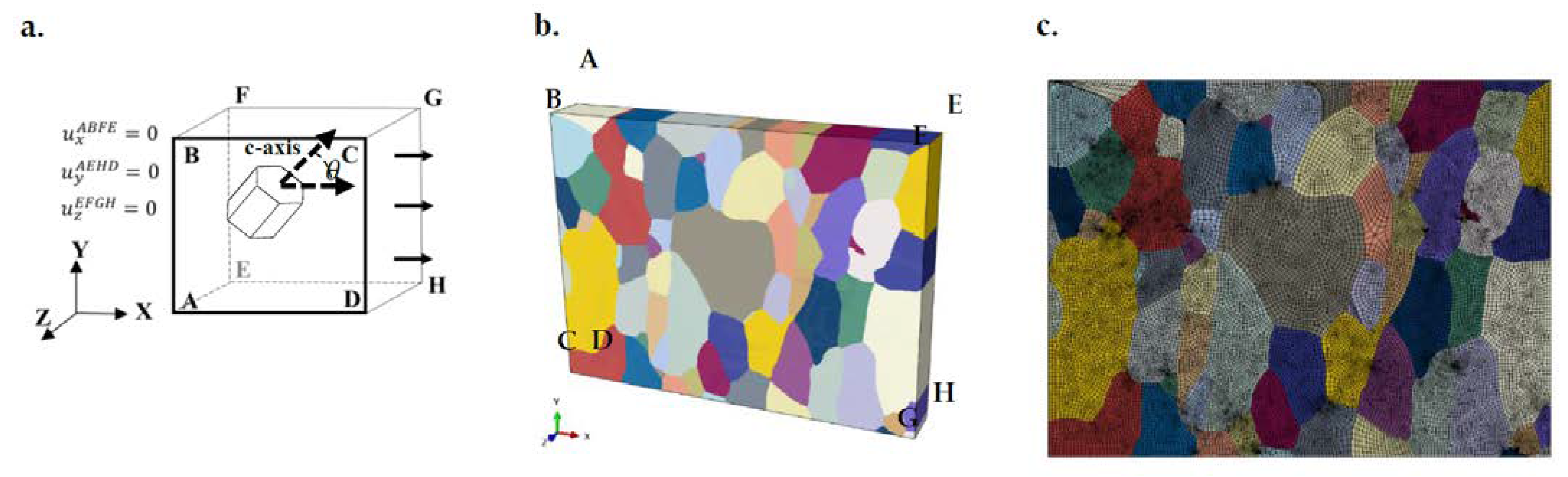
3.2. Input Models

3.2.1. Single Crystal

The evolution of GND and SSD densities as well as the CRSS of each slip system is studied using the single crystal model. This is to provide a comparison between the two methods used. A cube-shaped single crystal with a side length of 20 $\mathsf{\mu }\mathrm{m}$ is used for the FE input model. The cube is deformed uniaxially to 5% applied strain at the strain rate of 10⁻⁵ s⁻¹. Uniaxial tensile strain is applied on the surface DCGH along the X-direction (Figure 2a). Fixed displacement boundary conditions are applied on the ABFE, AEHD, and EFGH surfaces along X, Y, and Z directions, respectively. The model is discretized with 1000 quadratic brick elements with reduced integration points (C3D20R), with 10 elements in each direction. The c-axis of the HCP crystal was rotated with respect to the loading direction from 0° to 90° at the step size of 22.5°. As shown in Figure 2a, the misorientation between the loading direction and crystal c-axis is presented by θ.

3.2.2. Polycrystal

The measured EBSD map shown in Figure 1a is imported into the ABAQUS FE solver. The imported polycrystal model is shown in Figure 2. The as-measured strain and strain rates are applied to the FE model. The boundary conditions used are $u_x=0$ and $u_y=0$ on the ABCD and CGHD surfaces, respectively, and $u_z=0$ on the AD and DH edges. The model is extruded in the z direction to the thickness of 50 $\mathsf{\mu }\mathrm{m}$ to be consistent with the measured average grain size of the specimen. After conducting a mesh sensitivity study to ensure that FE results are converged, the model was discretized to 65,157 C3D20R brick elements. Three elements along the model thickness are used. The EBSD-measured grain orientations are assigned to each modeled grain. The model was deformed in two steps; in step 1, 1.2% uniaxial strain was applied to the model in the global x-direction, and in step 2, the model is unloaded and allowed to relax. In all simulations presented, the maximum time increment allowed is 5 s to ensure that the calculated GND densities are independent from the size of the selected time increment and are converged.

4. Results

A single crystal model is firstly used to calibrate the single crystal parameters for Method I of the CPFE model. This is followed by comparing the results of the CPFE models to those measured using HR-EBSD for stress, lattice rotations, and GND densities within the polycrystal. The capability of each method in determining slip activity and capturing slip bands is also discussed.

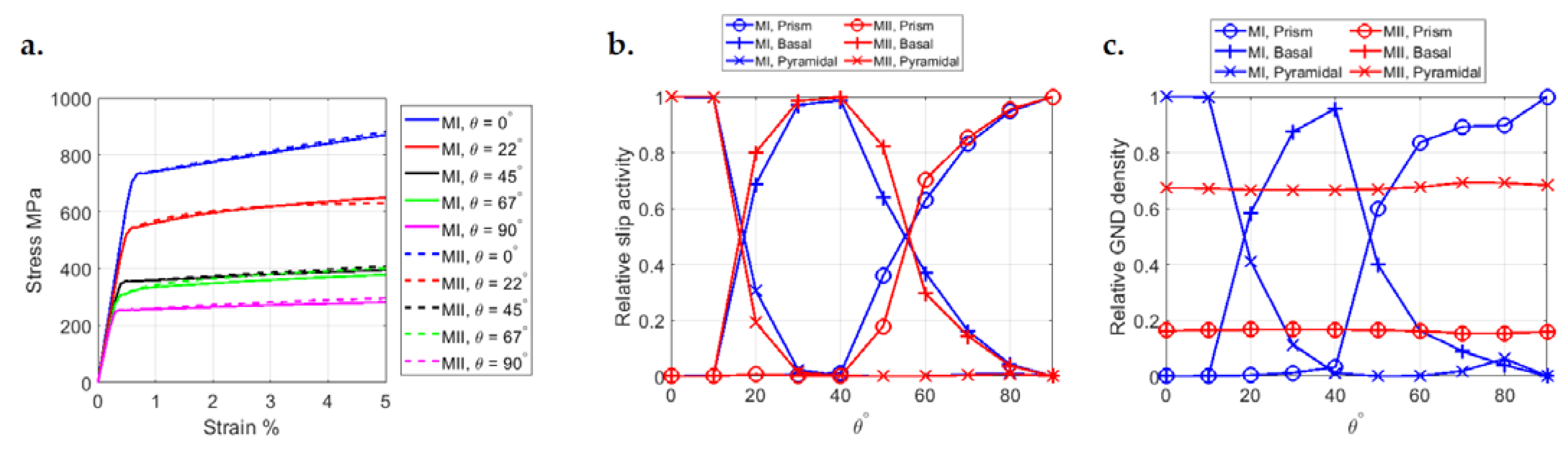
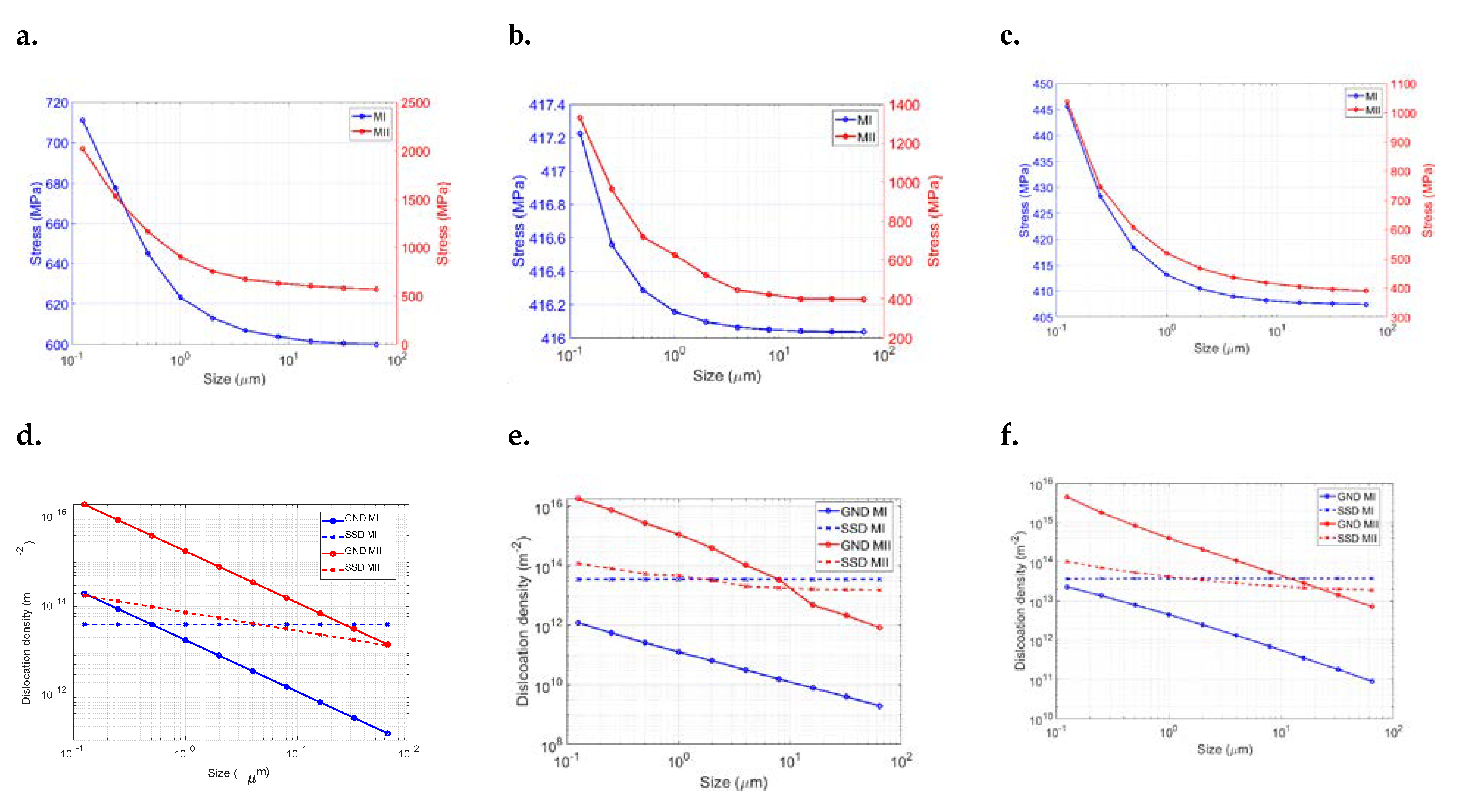
4.1. Single Crystal

The single crystal model shown in Figure 2a is used to calibrate the single crystal parameters for Method I of the CPFE model. The calculated stress of this method is compared to the one from Method II of the CPFE model. In addition, the calculated slip activities and GND densities are compared between the two methods. This is to understand the differences between each method at the single crystal level and to establish a foundation for the differences observed in the polycrystalline simulations.

In Figure 3a, the stress-strain curves calculated with the CPFE model using both Method I and II at five different crystal orientations are shown. In addition, the calculated relative activities of each slip system from both methods are provided in Figure 3b. Relative activities are the resolved shear strain (${\gamma }^{\alpha }$) for each slip set divided by the total shear strain at the applied strain of 5%. It is shown that identical stress-strain curves and slip activities are obtained for different crystal orientations.

Figure 3c compares the calculated relative GND density of each slip system from both methods of the CPFE model. Relative GND densities are determined by dividing the total GND density calculated for each slip set by the total GND density calculated for all slip systems. The calculated relative GND densities from Method I follow the same trends captured for the slip activities. However, the relative GND densities of Method II follow a nearly horizontal line, which is independent from the misorientation angle θ and the calculated slip system activity. Moreover, the relative GND density of the pyramidal slip system is almost four times higher than those from prism and basal slip systems. The relative GND densities calculated for prism and basal slip systems from Method II are identical. These two curves overlapp in Figure 3c. The relative GND densities calculated using Method II for each slip set is proportional to the number of variants for each slip set. That is, GND densities are evenly distributed on all variants of a slip system when Method II is used.

The evolution of the average GND and SSD densities of each slip set from the two methods implemented in the CPFE framework is compared in Figure 4. For each slip set, the total calculated dislocation density, either GND or SSD, is divided by the number of variants in the same slip set, i.e., M in $\frac{{{\displaystyle \sum }}_{\alpha =1}^M{\rho }_{GND}^{\alpha }}{M}$ is 3, 3, and 12 for prism, basal, and pyramidal slip systems, respectively. Results are for three different misorientation angles (θ). In addition, the calculated total dislocation densities, GNDs plus SSDs, from the two methods are compared. Although both methods predict identical average stress-strain curves (Figure 3a), a significant difference in the predicted GND densities is observed. The SSD and GND densities from Method II have the same order of magnitude. However, in Method I, SSD densities are at least two orders of magnitude higher than GND densities. This means that the hardening of slip systems from Method I is mainly driven by SSD densities as the contribution of GND densities is almost negligible. The cumulative dislocation densities calculated from both SSDs and GNDs are almost equal to those calculated from Method II. This results in calculating the same evolution for CRSS using both methods.

4.2. Polycrystal

Results presented in this section are from the CPFE model using both Method I and II. The CPFE results for GND densities are presented and compared to those measured via HR-EBSD. In addition, the capability of both methods in simulating formation of slip bands is evaluated by comparing the numerical results to those from SEM images of the deformed specimen. Finally, the distribution of calculated stresses and elastic lattice rotations are compared to those measured using HR-EBSD.

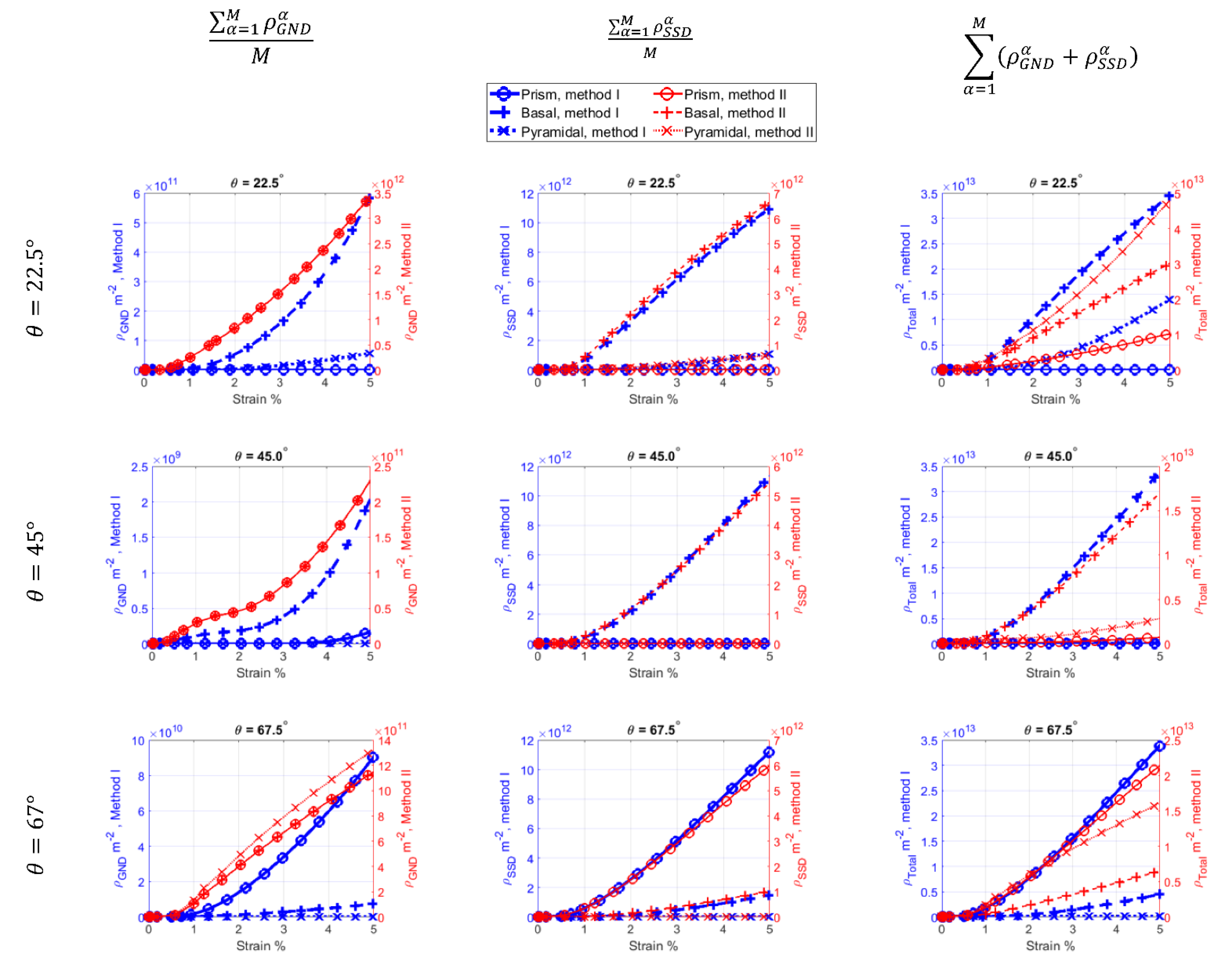
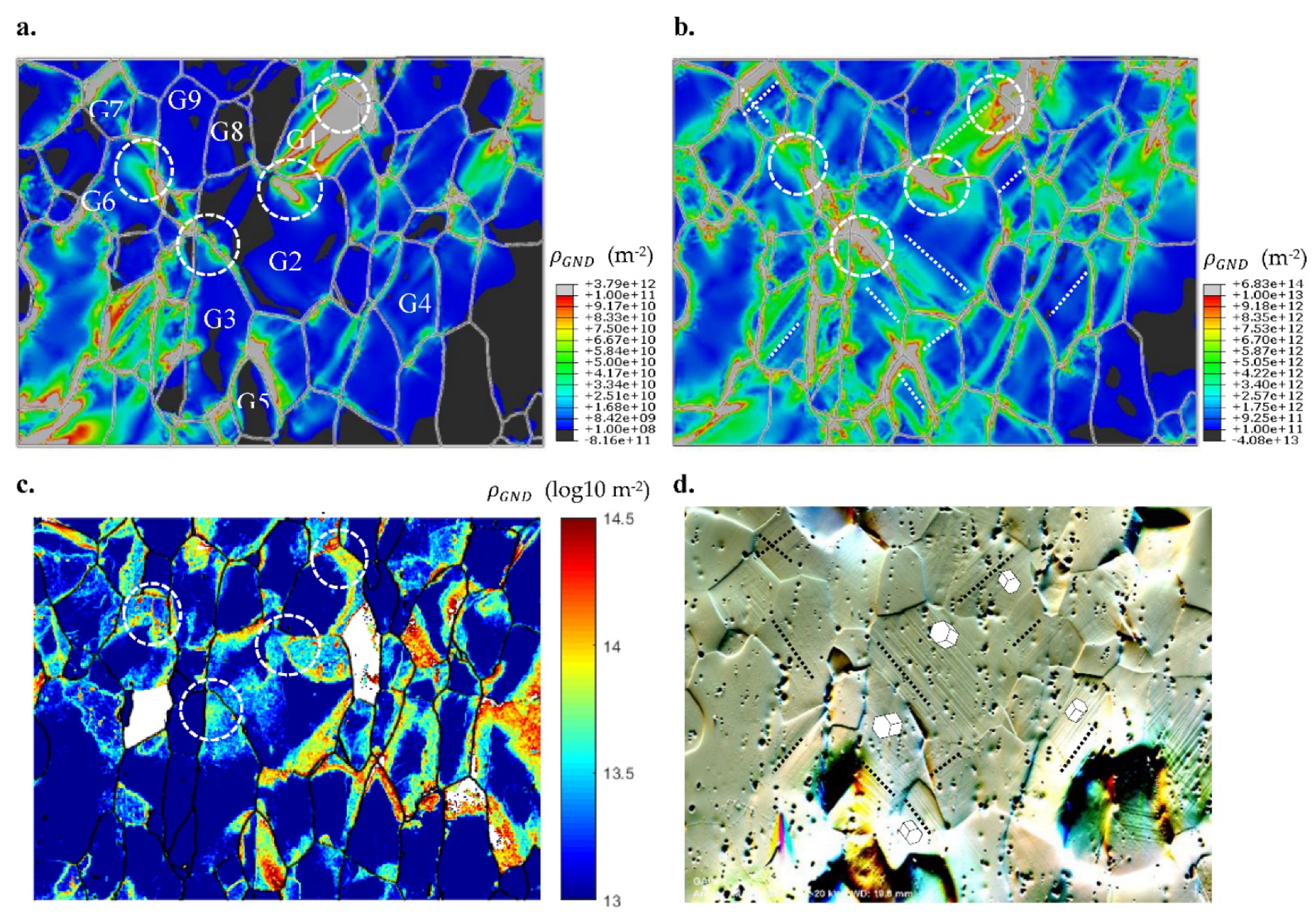
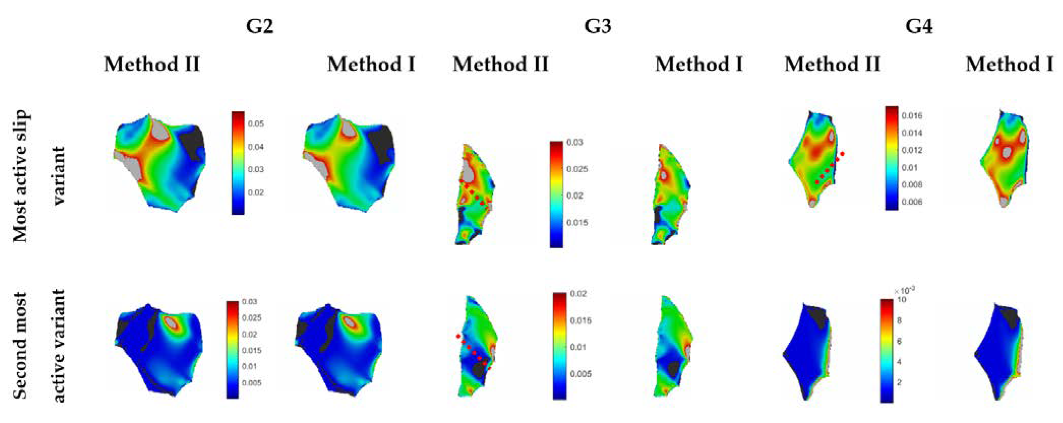
4.2.1. GND Density and Slip Activity

The distributions of total GND densities after the unload step for Method I and II are shown in Figure 5a,b, respectively. The total GND density from Method I is about an order of magnitude smaller than that calculated using Method II. For example, in grains G2, G3, and G5, marked in Figure 5a, a significant portion of the grains have GND densities lower than 10⁹ m⁻² when Method I is used. Moreover, the maximum GND density from Method I is about 4 × 10¹² m⁻², but it is ~7 × 10¹⁴ m⁻² when Method II is used. Although there is a noticeable difference in the magnitudes of calculated GNDs, the predicted trends are quite similar between the two methods. For example, most of the grain boundaries have high GND densities. In addition, both methods predict highly localized GND concentration sites at the top-right sections of grains G1 and G2, upper side of grain G3, and right side of grain G6. These areas are shown by the white circles in Figure 5a. HR-EBSD measurement also shows high GND density at these regions, as shown in Figure 5c. However, the magnitudes of GND densities from HR-EBSD are higher than those from both CPFE methods, but much closer to those from Method II. In comparison to Method I, the magnitude of GND densities from Method II is closer to those measured with HR-EBSD. This is not surprising because in the calculation of GND densities from HR-EBSD measurements, Method II is used along with the L¹ optimization scheme. As a result, it is expected to have a better agreement between HR-EBSD measurements for GNDs and those from Method II of the CPFE model. The effects of using L¹ and L² optimization schemes in determining GND densities from HR-EBSD are discussed elsewhere [59,60]. In addition, Method I cannot be used for HR-EBSD measurement as the plastic resolved shear strain on each slip system (${\gamma }^{\alpha }$) cannot be directly extracted with this technique (see Equation (10)).

Figure 5d shows an ARGUS image of the deformed polycrystal, in which slip bands can be observed in most of the grains. For better visualization, the orientations of slip bands are shown with the black dotted lines. Interestingly, CPFE results from both Method I and II also show GND density localization in the form of slip bands. For example, in grains G1, G2, G3, and G4, a distinct slip band is formed that spans from one side of the grain to another, as shown with the white dotted lines in Figure 5b. The orientations of these bands are in agreement with those observed in the SEM image in Figure 5d. In addition, both CPFE methods have captured the crossing of the two separate slip bands observed in grain G7. The two slip bands can also be observed in the ARGUS image. The CPFE results reveal that these slip bands are associated with the localization of plastic shear on the prism planes. This is also consistent with the measured grain orientations as shown in Figure 5d. For example, in grains G2, G3, and G4, the observed slip bands of the ARGUS image are parallel to ones of the variants of the prism planes of the illustrated HCP crystals. Therefore, both Method I and II are equally effective when predicting the direction of slip bands.

In order to determine the relationship between the observed slip bands and active slip systems, the average resolved shear strain and GND density of each slip set are extracted from the CPFE results and are shown in

Table 2. Average resolved shear strains and GND densities from the CPFE models. Results are for grains G1 to G5 of the polycrystalline model at 1.2% applied strain. The predominant slip system is shown in bold.

Grain ID	GND Method	Cumulative Resolved Shear Strain			GND Density m−2
		Prism	Basal	Pyr	Prism	Basal	Pyr	Total
1	I	4.8 × 10−2	3.6 × 10−3	<10−4	1.6 × 1011	1.5 × 109	1.3 × 106	1.6 × 1011
	II	4.4 × 10−2	2.4 × 10−3	<10−4	3.8 × 1011	3.8 × 1011	2.1 × 1012	2.9 × 1012
2	I	2.4 × 10−2	1.2 × 10−3	<10−4	3.7 × 109	1.4 × 108	4.1 × 105	3.9 × 109
	II	2.3 × 10−2	1.1 × 10−3	<10−4	1.8 × 1011	1.8 × 1011	9.1 × 1011	9.5 × 1011
3	I	7.0 × 10−2	3.2 × 10−2	<10−4	1.2 × 1010	1.4 × 1010	4.5 × 106	2.6 × 1010
	II	6.9 × 10−2	3.0 × 10−2	<10−4	1.9 × 1012	1.9 × 1012	8.8 × 1012	1.3 × 1013
4	I	1.1 × 10−1	5.5 × 10−3	<10−4	7.7 × 1010	5.1 × 109	9.2 × 107	8.2 × 1010
	II	1.2 × 10−1	5.3 × 10−3	<10−4	2.1 × 1012	2.1 × 1012	1.2 × 1013	1.6 × 1013
5	I	2.4 × 10−2	1.2 × 10−3	1.2 × 10−4	2.6 × 109	1.2 × 109	4.5 × 108	4.3 × 109
	II	2.3 × 10−2	0.9 × 10−3	1.1 × 10−4	4.2 × 1011	4.2 × 1011	2.5 × 1012	3.3 × 1012

. These values are calculated by taking the volume average of the resolved shear strains, or GNDs, calculated at all integration points assigned to each grain. The calculated average value for each slip set is the summation over all variants, i.e., 3 variants for basal or prism, and 12 variants for pyramidal <c + a>. Table 2 summarizes the amount of slip and GND density accumulated on the prism, basal, and pyramidal slip systems of grains G1 to G5. The predominant slip system with the highest value is presented in bold. Both methods confirm that the predominant slip system for all five selected grains is slip on the prism planes. For example, for grain G4 almost all plastic deformation is accommodated by prism slip systems whereas for grain G3 both basal and prism slip systems are active with prism being the most active one. Although these trends are also observed for the GND densities obtained from Method I, the pyramidal slip system accommodates most of the GNDs calculated in Method II. In fact, the GND density from method II is almost evenly distributed on all eighteen variants, but since the pyramidal slip system has 12 variants, it always has the highest GND density once the summation is done over all 12 variants. These results are consistent with the trends observed for the single crystal model. The heterogeneous distribution of the GND densities on the different slip variants in Method I is more reasonable compared to Method II, where the GND densities on individual slip variants are always equal, regardless of the applied loading conditions.

Figure 6 shows the distribution of resolved shear strains on the first and second most active slip variants. Results are for grains G2, G3, and G4. All variants are related to the slip on prism, except for grain G3 where its second dominant variant belongs to the basal system (see Table 2). Shear strain localization in the form of slip bands is observed in all three grains. These slip bands are shown with a red dotted lines in Figure 6. These bands are parallel to the ones observed in the GND maps in Figure 5a,b as well as those observed in the ARGUS image of Figure 5d.

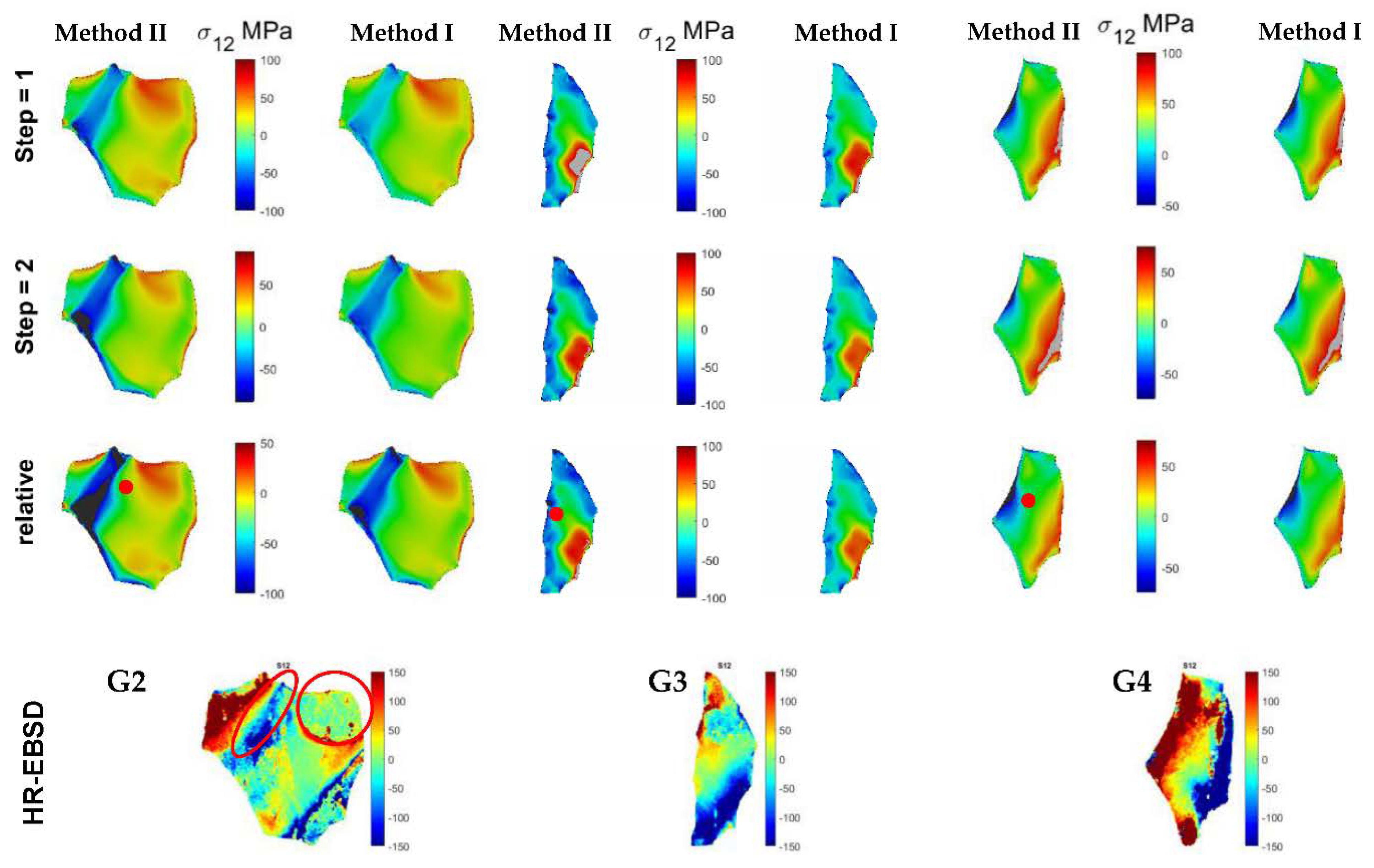
4.2.2. Stress

The normal stress component along the loading direction (${\sigma }_{11}$) and the in-plane shear stress component (${\sigma }_{12}$) of grains G3, G4, and G5 are shown in Figure 7 and Figure 8, respectively. The distribution of ${\sigma }_{11}$ is almost identical between Method I and II. After unloading, the normal stress drops significantly. The distributions of ${\sigma }_{11}$ from HR-EBSD are also shown in the last row of Figure 7. In an HR-EBSD measurement, a reference point is selected within each grain to measure “relative” stresses and elastic lattice rotations with respect to this point. These reference points are shown with the red dots in Figure 7. Since stresses from HR-EBSD are relative, the calculated stresses at all integration points assigned to a grain are reduced from those calculated at the integration point that coincides with the HR-EBSD reference point. This is to provide a like-to-like comparison between CPFE results and the HR-EBSD measurement.

For grain G2 of Figure 7, a tensile stress field is predicted in the lower half of the grain where the stress magnitude increases toward the grain boundary. This is in agreement with HR-EBSD measurement. In addition, two compressive stress fields are observed in the upper half of the grain. In comparison to the measurement, the size of these two fields is overestimated in CPFE results, although the trends are the same. Grain G3 can be divided into three regions, i.e., top, bottom, and middle regions. Calculated stress ${\sigma }_{11}$ is tensile in the top and bottom regions, while it is compressive in the middle region. This is in agreement with the HR-EBSD measurement. For grain G4, the left side of the grain has a compressive stress field, and the bottom side of the grain has a tensile stress field in both the model and experiment.

In Figure 8, it is shown that the distribution of shear stress ${\sigma }_{12}$ is nearly identical between Method I and II. For grain G2, a negative shear stress band is observed in the CPFE results on the top-left side of the grain. This band is also observed in the HR-EBSD measurement. In addition, a positive ${\sigma }_{12}$ region, at the top-right side of the grain, is calculated in both CPFE models, which is also observed in the HR-EBSD measurement. However, there are regions in grains G3 and G4 where the calculated shear stress ${\sigma }_{12}$ does not match with those from the HR-EBSD measurement. The magnitude and distribution of calculated normal (Figure 7) and shear stresses (Figure 8) are quite similar between the Method I and II.

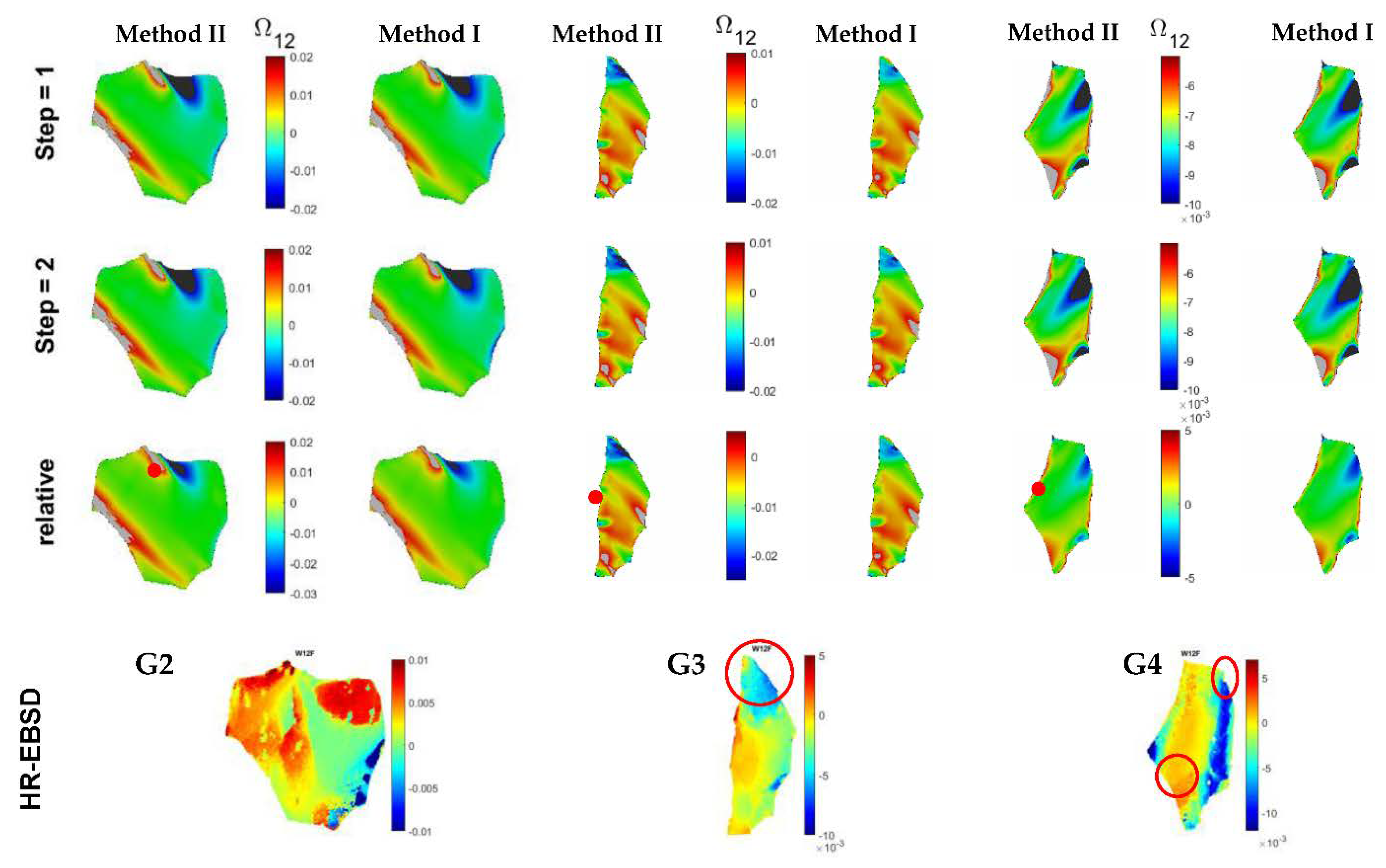
4.2.3. Lattice Rotations

The in-plane elastic rotation component of grains G2, G3, and G4 are shown in Figure 9 and the results of Method I and II are compared with those from HR-EBSD. Since measurements were done at the surface, only the in-plane component of the lattice rotation (${\mathsf{\Omega }}_{12}^e$) is shown. The relative values with respect to the reference point are presented in the last row of the simulation results. No difference is observed between the two methods in all the three grains after the loading and unloading steps. This means that although different GND densities are calculated in these two methods, the parameters are calibrated well, such that the resulting deformation tensors are almost identical from the two methods. The relative values with respect to the reference point of the EBSD follow the same trend as the HR-EBSD measurement. For example, both CPFE and HR-EBSD results show positive elastic rotation ${\mathsf{\Omega }}_{12}$ in the left half of grain G2. In addition, in both the model and experiment, the top side of grain G3 has negative elastic rotation ${\mathsf{\Omega }}_{12}$. Furthermore, the CPFE results show negative ${\mathsf{\Omega }}_{12}$ on the top-right side and positive ${\mathsf{\Omega }}_{12}$ on the lower left side of grain G4, which agrees with the HR-EBSD measurement.

5. Discussion

A lower-order strain-gradient crystal plasticity finite element model was developed in which two different methods were used to describe the evolution of GND densities. In Method I, a definite value was calculated for the magnitude of GNDs on each slip system, whereas in Method II, a minimization approach was used to solve for an under-determined system of equations. The performance of CPFE models was examined both for single crystal models and for polycrystalline models. In addition, the as-measured microstructure of a deformed α-zirconium sample was imported to the FE solver to compare the calculated grain-scale stresses, elastic lattice rotations, and GNDs to those measured using HR-EBSD.

Results shown in all previous sections were for single or polycrystalline models with an average grain size of more than 20 µm. The results of the strain-gradient CPFE model, however, are length-scale-dependent and are highly sensitive to the size of the studied grains [47]. Such a size dependency originates from the accumulated GND density, which is a function of plastic strain gradients. Since the magnitudes of GND densities from Method I and II are very different, it is important to check the effects of grain size on the results obtained. To do so, the single crystal model used in Section 3.1 is also used here, but the model is scaled so that different grain sizes can be studied. The model is scaled to ten different sizes from 0.125 µm to 64 µm and the calculated stresses, GND, and SSD densities from Method I and II are compared. The misorientation between the c-axis of the grain and the loading direction is set at 22.5°, 45°, and 67.5°. The macroscopic strain applied to the polycrystal is 5%. The Hall-Petch effects are switched off to only study the geometrical effects on the material hardening.

Figure 10a–c show that the average stress for the single crystal with a misorientation angle of 22.5°, 45°, 67.5°, respectively. It is shown that the stress magnitude is highly affected by the model size when Method II is used, particularly when the grain size is smaller than 10 µm. Although Method I also shows some dependency on the grain size, the magnitude of the stress is only significantly affected by the grain size for the grains smaller than 1 µm. This is the reason why the stresses obtained from the two methods for the polycrystal, presented in Section 4.2.2 with an average grain size of 50 µm, are not that different. Figure 10d–f show that the average GND and SSD density for the single crystal with a misorientation angle of 22.5°, 45°, 67.5°, respectively. It is shown that the calculated GND density has a linear relation with the grain size in the log-log scale. Interestingly, the slopes of these two lines are the same for the two methods used. In contrast to GNDs, SSDs are almost unaffected by the grain size. Therefore, the hardening of bigger grains is SSD driven, while that of smaller grains is GND driven. This means that SSDs are as important in determining stress development. Hence, when the formulation provided here is used to study fracture of polycrystals at grain scale [31,32], it is very important to fully characterize the contribution of both GNDs and SSDs to material plastic deformation.

A lower-order strain-gradient crystal plasticity model is used here, where the material hardening law is modified by including the strain gradient terms. One of the disadvantages of this approach is the formation of unrealistic, localized deformation fields as described in [16]. Further, when lower-order formulation is used, CPFE results are mesh-size dependent; on the other hand, when higher-order formulation is used, CPFE results are almost mesh independent [61].

The simulation results obtained from CPFE models showed several discrepancies with respect to those from HR-EBSD. The observed discrepancies could be due to ignoring the sub-surface grain structures in the CPFE results. As shown in Figure 2, a columnar grain structure was assumed in the CPFE model by extruding the measured EBSD map along the z-axis. This is because the EBSD measurement provides the information about the sub-surface grains. Although ignoring the sub-surface grain structures may affect the stress values at the free surface in the CPFE results [62,63,64], Zhang et al. showed that the calculated trends in the GND densities and strains are not much affected by the sub-surface microstructure [48].

Table 3. A comparison between Method I and II for determining GND densities.

Implementation	Lower-order non-local CPFE	Both methods can be implemented, but the implementation of Method I is more straightforward than Method II
	Higher-order non-local CPFE	Only Method I
Performance	Total GND density	Results from Method II are closer to those measured with HR-EBSD.
	GND density on each slip system	Method I: the calculated values are proportional to the cumulative slip for each slip variant Method II: almost equal for all slip systems

summarizes the results of the comparisons made between Method I and II. The effectiveness of the two methods can be assessed using two different perspectives: implementation and performance. From the implementation point of view, Method I is more straightforward and can be used for developing higher-order non-local CPFE models. This method is also computationally efficient since no optimization is required to determine the density of GNDs. In terms of performance, the use of Method II leads to closer numbers to those measured with HR-EBSD for GND density but results in uniform distribution of GNDs on all slip variants. Finally, when larger grain sizes are used, typically more than 10 µm, there is no difference between the two methods.

6. Conclusions

A user material (UMAT) subroutine is updated to include the strain-gradient effects. Two different methods are used for determining GND densities. The performance of the two methods for simulating the formation of slip bands in a deformed α-zirconium specimen is investigated. Numerical results are compared with those measured with HR-EBSD. It is shown that:

• The GND maps calculated from the strain-gradient CPFE models using both methods show formation of localized GND lines within the grains of the polycrystal. These GND lines are parallel to the slip bands observed in the deformed specimen using electron microscopy. The slip bands can also be seen in the CPFE-calculated shear strain maps.
• The use of the minimization-based approach for the determination of GND densities (Method II) leads to a uniform distribution of GNDs on all slip systems, whereas when the direct approach (Method I) is used, the magnitude of the calculated GNDs on each slip system is proportional to the plastic shear strain accumulated on the same slip system.
• Although the magnitudes of GND densities are different from the two methods, the trends observed for the calculated grain-scale stresses and lattice rotations are the same. This is because for the studied microstructure, where the average grain size is 50 µm, the calculated total dislocation density, GND plus SSD, from the two methods is almost the same.
• When a smaller grain size is used, the calculated average stresses from the two methods are different. The critical grain size below which the geometrical effects become significant is higher in Method II, compared to Method I.
• The dislocation-based hardening law used here is SSD driven for larger grains and GND driven for smaller grains, and accurate implementation of both mechanisms is important when different grain sizes exist in the microstructure.

The formation of the slip bands can also be simulated using higher-order strain-gradient crystal plasticity models. The incorporation of higher order terms to the CPFE model is in the scope of our future studies.

References

- Rovinelli, A.; Proudhon, H.; Lebensohn, R.A.; Sangid, M.D. Assessing the reliability of fast Fourier transform-based crystal plasticity simulations of a polycrystalline material near a crack tip. Int. J. Solids Struct. 2020, 184, 153–166. [Google Scholar] [CrossRef]
- Petkov, M.P.; Hu, J.; Tarleton, E.; Cocks, A.C.F. Comparison of self-consistent and crystal plasticity FE approaches for modelling the high-temperature deformation of 316H austenitic stainless steel. Int. J. Solids Struct. 2019, 171, 54–80. [Google Scholar] [CrossRef]
- Ma, R.; Truster, T.J.; Puplampu, S.B.; Penumadu, D. Investigating mechanical degradation due to fire exposure of aluminum alloy 5083 using crystal plasticity finite element method. Int. J. Solids Struct. 2018, 134, 151–160. [Google Scholar] [CrossRef]
- Lu, X.; Zhang, X.; Shi, M.; Roters, F.; Kang, G. Dislocation mechanism based size-dependent crystal plasticity modeling and simulation of gradient nano-grained copper. Int. J. Plast. 2019, 113, 52–73. [Google Scholar] [CrossRef]
- Han, F.; Roters, F.; Raabe, D. Microstructure-based multiscale modeling of large strain plastic deformation by coupling a full-field crystal plasticity-spectral solver with an implicit finite element solver. Int. J. Plast. 2020, 125, 97–117. [Google Scholar] [CrossRef]
- Kasemer, M.; Dawson, P. A finite element methodology to incorporate kinematic activation of discrete deformation twins in a crystal plasticity framework. Comput. Methods Appl. Mech. Eng. 2020, 358, 1–29. [Google Scholar] [CrossRef]
- Wijnen, J.; Peerlings, R.H.J.; Hoefnagels, J.P.M.; Geers, M.G.D. A discrete slip plane model for simulating heterogeneous plastic deformation in single crystals. Int. J. Solids Struct. 2021, 228, 111094. [Google Scholar] [CrossRef]
- Nemat-nasser, S.; Ni, L.; Okinaka, T. A constitutive model for fcc crystals with application to polycrystalline OFHC copper. Mech. Mater. 1998, 30, 325–341. [Google Scholar] [CrossRef]
- Kocks, U.F.; Argon, A.S.; Ashby, M.F. Thermodynamics and Kinetics of Slip; Pergamon Press: Cambridge, UK, 1975. [Google Scholar]
- Evers, L.P.; Brekelmans, W.A.M.; Geers, M.G.D. Non-local crystal plasticity model with intrinsic SSD and GND effects. J. Mech. Phys. Solids 2004, 52, 2379–2401. [Google Scholar] [CrossRef]
- Ashby, M.F. The deformation of plastically non-homogeneous materials. Philos. Mag. 1970, 21, 399–424. [Google Scholar] [CrossRef]
- Taylor, G.I. The Mechanism of Plastic Deformation of Crystals. Part 1. Theoretical. Proc. R. Soc. 1934, 538, 362–387. [Google Scholar]
- Arsenlis, A.; Parks, D.M. Modeling the evolution of crystallographic dislocation density in crystal plasticity. J. Mech. Phys. Solids 2002, 50, 1979–2009. [Google Scholar] [CrossRef]
- Arsenlis, A.; Parks, D.M.; Becker, R.; Bulatov, V.V. On the evolution of crystallographic dislocation density in non-homogeneously deforming crystals. J. Mech. Phys. Solids 2004, 52, 1213–1246. [Google Scholar] [CrossRef]
- Gurtin, M.E. A gradient theory of single-crystal viscoplasticity that accounts for geometrically necessary dislocations. J. Mech. Phys. Solids 2002, 50, 5–32. [Google Scholar] [CrossRef]
- Niordson, C.F.; Hutchinson, J.W. On lower order strain gradient plasticity theories. Eur. J. Mech. A/Solids 2003, 22, 771–778. [Google Scholar] [CrossRef]
- Bassani, J.L. Incompatibility and a simple gradient theory of plasticity. J. Mech. Phys. Solids 2001, 49, 1983–1996. [Google Scholar] [CrossRef]
- Busso, E.P.; Meissonnier, F.T.; Dowd, N.P.O. Gradient-dependent deformation of two-phase single crystals. J. Mech. Phys. Solids 2000, 48, 2333–2361. [Google Scholar] [CrossRef]
- Arsenlis, A.; Parks, D.M. Crystallographic aspects of geometrically nesesary and statistically stored dislocation density. Acta Mater. 1999, 47, 1597–1611. [Google Scholar] [CrossRef]
- De Borst, R.; Mühlhaus, H.-B. Gradient-dependent plasticity: Formulation and algorithmic aspects. Int. J. Numer. Methods Eng. 1992, 35, 521–539. [Google Scholar] [CrossRef] [Green Version]
- Gao, H.; Huang, Y.; Nix, W.D.; Hutchinson, J.W. Mechanism-based strain gradient plasticity—I. Theory. J. Mech. Phys. Solids 1999, 47, 1239–1263. [Google Scholar] [CrossRef]
- Yun, G.; Hwang, K.C.; Huang, Y.; Wu, P.D. A reformulation of mechanism-based strain gradient plasticity. Philos. Mag. 2005, 85, 4011–4029. [Google Scholar] [CrossRef]
- Gurtin, M.E. On the plasticity of single crystals: Free energy, microforces, plastic-strain gradients. J. Mech. Phys. Solids 2000, 48, 989–1036. [Google Scholar] [CrossRef]
- Nye, J. Some geometrical relations in dislocated crystals. Acta Metall. 1953, 1, 153–162. [Google Scholar] [CrossRef]
- Das, S.; Hofmann, F.; Tarleton, E. Consistent determination of geometrically necessary dislocation density from simulations and experiments. Int. J. Plast. 2018, 109, 18–42. [Google Scholar] [CrossRef]
- Dai, H. Geometrically-Necessary Dislocation Density in Continuum Plasticity Theory. Ph.D. Thesis, Massachusetts Institute of Technology, Cambridge, MA, USA, 1997. [Google Scholar]
- Ma, A.; Roters, F.; Raabe, D. A dislocation density based constitutive model for crystal plasticity FEM including geometrically necessary dislocations. Acta Mater. 2006, 54, 2169–2179. [Google Scholar] [CrossRef]
- Dunne, F.P.E.; Rugg, D.; Walker, A. Lengthscale-dependent, elastically anisotropic, physically-based hcp crystal plasticity: Application to cold-dwell fatigue in Ti alloys. Int. J. Plast. 2007, 23, 1061–1083. [Google Scholar] [CrossRef]
- Waheed, S.; Zheng, Z.; Balint, D.S.; Dunne, F.P.E. Microstructural effects on strain rate and dwell sensitivity in dual-phase titanium alloys. Acta Mater. 2019, 162, 136–148. [Google Scholar] [CrossRef]
- Arsenlis, A. Modeling Dislocation Density Evolution in Continuum Crystal Plasticity. Available online: http://dspace.mit.edu/handle/1721.1/36679%5Cnhttps://dspace.mit.edu/handle/1721.1/36679 (accessed on 16 July 2001).
- Chen, B.; Jansenss, K.; Dunne, F.P.E. Role of geometrically necessary dislocation density in multiaxial and non-proportional fatigue crack nucleation. Int. J. Fatigue 2020, 135, 105517. [Google Scholar] [CrossRef]
- Wilson, D.; Dunne, F.P.E. A mechanistic modelling methodology for microstructure-sensitive fatigue crack growth. J. Mech. Phys. Solids 2019, 124, 827–848. [Google Scholar] [CrossRef]
- Dunne, F.P.E.; Kiwanuka, R.; Wilkinson, A.J. Crystal plasticity analysis of micro-deformation, lattice rotation and geometrically necessary dislocation density. Proc. R. Soc. A Math. Phys. Eng. Sci. 2012, 468, 2509–2531. [Google Scholar] [CrossRef] [Green Version]
- Cheng, J.; Ghosh, S. A crystal plasticity FE model for deformation with twin nucleation in magnesium alloys. Int. J. Plast. 2015, 67, 148–170. [Google Scholar] [CrossRef]
- Wu, W.; An, K.; Huang, L.; Lee, S.Y.; Liaw, P.K. Deformation dynamics study of a wrought magnesium alloy by real-time in situ neutron diffraction. Scr. Mater. 2013, 69, 358–361. [Google Scholar] [CrossRef]
- Xu, F.; Holt, R.A.; Daymond, M.R.; Rogge, R.B.; Oliver, E.C. Development of internal strains in textured Zircaloy-2 during uni-axial deformation. Mater. Sci. Eng. A 2008, 488, 172–185. [Google Scholar] [CrossRef]
- Louca, K.; Abdolvand, H. Accurate determination of grain properties using three-dimensional synchrotron X-ray diffraction: A comparison with EBSD. Mater. Charact. 2021, 171, 110753. [Google Scholar] [CrossRef]
- Abdolvand, H.; Louca, K.; Mareau, C.; Majkut, M.; Wright, J. On the nucleation of deformation twins at the early stages of plasticity. Acta Mater. 2020, 196, 733–746. [Google Scholar] [CrossRef]
- Abdolvand, H.; Wright, J.P.; Wilkinson, A.J. On the state of deformation in a polycrystalline material in three-dimension: Elastic strains, lattice rotations, and deformation mechanisms. Int. J. Plast. 2018, 106, 145–163. [Google Scholar] [CrossRef]
- Wallis, D.; Parsons, A.J.; Hansen, L.N. Quantifying geometrically necessary dislocations in quartz using HR-EBSD: Application to chessboard subgrain boundaries. J. Struct. Geol. 2019, 125, 235–247. [Google Scholar] [CrossRef]
- Ungar, T.; Drakopoulos, M.; Be, J.L.; Chauveau, T.; Castelnau, O.; Riba, G.; Snigirev, A.; Snigireva, I.; Schroer, C.; Bacroix, B. Grain to grain slip activity in plastically deformed Zr determined by X-ray micro-diffraction line profile analysis. Acta Mater. 2007, 55, 1117–1127. [Google Scholar] [CrossRef]
- Wilkinson, A.J.; Meaden, G.; Dingley, D.J. High-resolution elastic strain measurement from electron backscatter diffraction patterns: New levels of sensitivity. Ultramicroscopy 2006, 106, 307–313. [Google Scholar] [CrossRef] [PubMed]
- Wilkinson, A.J. Measurement of elastic strains and small lattice rotations using electron back scatter diffraction. Ultramicroscopy 1996, 62, 237–247. [Google Scholar] [CrossRef]
- Troost, K.Z.; Van Der Sluis, P.; Gravesteijn, D.J. Microscale elastic-strain determination by backscatter Kikuchi diffraction in the scanning electron microscope. Appl. Phys. Lett. 1993, 62, 1110–1112. [Google Scholar] [CrossRef]
- Guo, Y.; Abdolvand, H.; Britton, T.B.; Wilkinson, A.J. Growth of {112¯2} twins in titanium: A combined experimental and modelling investigation of the local state of deformation. Acta Mater. 2017, 126, 221–235. [Google Scholar] [CrossRef]
- Britton, T.B.; Wilkinson, A.J. High resolution electron backscatter diffraction measurements of elastic strain variations in the presence of larger lattice rotations. Ultramicroscopy 2012, 114, 82–95. [Google Scholar] [CrossRef] [PubMed]
- Sedaghat, O.; Abdolvand, H. A non-local crystal plasticity constitutive model for hexagonal close-packed polycrystals. Int. J. Plast. 2021, 136, 102883. [Google Scholar] [CrossRef]
- Zhang, Z.; Lunt, D.; Abdolvand, H.; Wilkinson, A.J.; Preuss, M.; Dunne, F.P.E. Quantitative investigation of micro slip and localization in polycrystalline materials under uniaxial tension. Int. J. Plast. 2018, 108, 88–106. [Google Scholar] [CrossRef] [Green Version]
- Abdolvand, H.; Sedaghat, O.; Guo, Y. Nucleation and growth of {112¯2} twins in titanium: Elastic energy and stress fields at the vicinity of twins. Materialia 2018, 2, 58–62. [Google Scholar] [CrossRef]
- Abdolvand, H.; Wright, J.; Wilkinson, A.J. Strong grain neighbour effects in polycrystals. Nat. Commun. 2018, 9, 171. [Google Scholar] [CrossRef] [Green Version]
- Abdolvand, H.; Wilkinson, A.J. On the effects of reorientation and shear transfer during twin formation: Comparison between high resolution electron backscatter diffraction experiments and a crystal plasticity finite element model. Int. J. Plast. 2016, 84, 160–182. [Google Scholar] [CrossRef] [Green Version]
- Asaro, R.J.; Needleman, A. Overview No. 42 Texture development and strain hardening in rate dependent polycrystals. Acta Metall. 1985, 33, 923–953. [Google Scholar] [CrossRef]
- Asaro, R.J. Crystal Plasticity. J. Appl. Mech. 1983, 50, 921–934. [Google Scholar] [CrossRef]
- Fisher, E.S.; Renken, C.J. Single-crystal elastic moduli and the hcp → bcc transformation in Ti, Zr, and Hf. Phys. Rev. 1964, 135, A482–A494. [Google Scholar] [CrossRef]
- Beyerlein, I.J.; Tomé, C.N. A dislocation-based constitutive law for pure Zr including temperature effects. Int. J. Plast. 2008, 24, 867–895. [Google Scholar] [CrossRef]
- Cheong, K.S.; Busso, E.P.; Arsenlis, A. A study of microstructural length scale effects on the behaviour of FCC polycrystals using strain gradient concepts. Int. J. Plast. 2005, 21, 1797–1814. [Google Scholar] [CrossRef] [Green Version]
- Abdolvand, H. Progressive modelling and experimentation of hydrogen diffusion and precipitation in anisotropic polycrystals. Int. J. Plast. 2019, 116, 39–61. [Google Scholar] [CrossRef]
- Abdolvand, H.; Daymond, M.R.; Mareau, C. Incorporation of twinning into a crystal plasticity finite element model: Evolution of lattice strains and texture in Zircaloy-2. Int. J. Plast. 2011, 27, 1721–1738. [Google Scholar] [CrossRef]
- Wallis, D.; Hansen, L.N.; Britton, T.B.; Wilkinson, A.J. High-Angular Resolution Electron Backscatter Diffraction as a New Tool for Mapping Lattice Distortion in Geological Minerals. J. Geophys. Res. Solid Earth 2019, 124, 6337–6358. [Google Scholar] [CrossRef]
- Wallis, D.; Hansen, L.N.; Ben Britton, T.; Wilkinson, A.J. Geometrically necessary dislocation densities in olivine obtained using high-angular resolution electron backscatter diffraction. Ultramicroscopy 2016, 168, 34–45. [Google Scholar] [CrossRef] [Green Version]
- Kuroda, M.; Tvergaard, V. Studies of scale dependent crystal viscoplasticity models. J. Mech. Phys. Solids 2006, 54, 1789–1810. [Google Scholar] [CrossRef]
- Baudoin, P.; Hama, T.; Takuda, H. Influence of critical resolved shear stress ratios on the response of a commercially pure titanium oligocrystal: Crystal plasticity simulations and experiment. Int. J. Plast. 2019, 115, 111–131. [Google Scholar] [CrossRef]
- Zeghadi, A.; Forest, S.; Gourgues, A.F.; Bouaziz, O. Ensemble averaging stress-strain fields in polycrystalline aggregates with a constrained surface microstructure-part 2: Crystal plasticity. Philos. Mag. 2007, 87, 1425–1446. [Google Scholar] [CrossRef]
- St-Pierre, L.; Héripré, E.; Dexet, M.; Crépin, J.; Bertolino, G.; Bilger, N. 3D simulations of microstructure and comparison with experimental microstructure coming from O.I.M analysis. Int. J. Plast. 2008, 24, 1516–1532. [Google Scholar] [CrossRef]